Scaling and criticality of the Kondo effect in a Luttinger liquid

Abstract

A quantum Monte Carlo simulation method has been developed and applied to study the critical behavior of a single Kondo impurity in a Luttinger liquid. This numerically exact method has no finite-size limitations and allows to simulate the whole temperature range. Focusing on the impurity magnetic susceptibility, we determine the scaling functions, in particular for temperatures well below the Kondo temperature. In the absence of elastic potential scattering, we find Fermi-liquid behavior for strong electron-electron interactions, $g_{c}<1/2$, and anomalous power laws for $1/2<g_{c}<1$, where $g_{c}$ is the correlation parameter of the Luttinger liquid. These findings resolve a recent controversy. If elastic potential scattering is present, we find a logarithmically divergent impurity susceptibility at $g_{c}<1/2$ which can be rationalized in terms of the two-channel Kondo model.

I Introduction

Since its discovery, the Kondo problem is one of the central topics in condensed-matter physics.[1, 2] It describes a magnetic spin-$\frac{1}{2}$ impurity embedded into a metal and may be the simplest example for the growth of an effective coupling at low energies, resulting in a nonperturbative ground state. For normal metals this ground state is found to be of Fermi-liquid type, where the quasi-particle wave functions simply acquire a phase shift.[3] The situation might change in one-dimensional (1D) systems which are known to exhibit non-Fermi liquid behavior for arbitrary Coulomb interactions. The fundamental theory of interacting 1D metals in the low-energy regime is the Luttinger liquid model.[4, 5, 6] It is therefore of interest to understand the Kondo effect in a Luttinger liquid. An additional motivation arises from recent advances in nanofabrication which now allow for controlled experiments on 1D systems.[7] In the future the question of how magnetic impurities behave when coupled to 1D metals might be of crucial importance for experiments on quantum wires,[7, 8] carbon nanotubes,[9] or for edge states in the fractional quantum Hall regime.[10]

The Luttinger liquid model unifies the low-temperature physics of many microscopic lattice models for strongly correlated fermions, with only very few phenomenological parameters. In particular, one has the dimensionless Coulomb interaction strength parameters $g_{c}$ and $g_{s}$ for charge and spin sectors, respectively, and the charge- and spin-density velocities $v_{c}$ and $v_{s}$. The crucial assumptions are the absence of lattice instabilities (like Umklapp scattering), the absence of electron-electron backscattering, and that the Coulomb interaction potential is screened by mobile charge carriers close to the 1D metal. As a simple model for interacting fermions, the Luttinger liquid model is widely used to study the influence of electronic correlations on dynamical properties of 1D metals, in particular in the presence of impurities. The case of a spinless impurity is by now well understood.[11] If the impurity has internal degrees of freedom, the situation is more complicated and subject of this paper.

A Kondo impurity coupled to a Luttinger liquid was first considered by Lee und Toner.[12] Employing the perturbative renormalization group they established how the Kondo temperature $T_{K}$ depends on the exchange coupling constant $J$. This turns out to be a power-law dependence, while for normal metals $T_{K}$ is an exponential function of the coupling constant.[2] The same power law was found by Furusaki and Nagaosa.[13] These authors derived the correct $SU(2)$ invariant scaling equations in the weak-coupling regime and tentatively extended them to the strong-coupling regime, where a stable strong-coupling fixed point was found for both antiferromagnetic and ferromagnetic exchange couplings. This strong-coupling fixed point describes a many-body singlet formed by the impurity spin and the conduction electrons, similar to what happens in a normal metal. Moreover, Furusaki and Nagaosa made detailed predictions concerning the low-temperature critical properties of the impurity, e.g., the magnetic susceptibility, the heat capacity, and the conductance. These quantities were found to exhibit power-law behavior with interaction-dependent exponents.

However, it remained unclear whether the extrapolation of the perturbative scaling equations into the strong-coupling regime is justified. Recent boundary conformal field theory (CFT) results by Fröjdh and Johannesson[14] allow only two possible scenarios. Either the system belongs to the Fermi liquid universality class or it indeed has the properties predicted by Furusaki and Nagaosa. CFT itself is however unable to unambiguously decide which universality class is ultimately realized for the Kondo problem in a Luttinger liquid. Several recent papers seem to favor the local Fermi-liquid picture. Schiller and Ingersent have discussed a truncated but related model which exhibits Fermi-liquid behavior.[15] In addition, according to the numerical density-matrix renormalization group (DMRG) calculation of Wang,[16] Fermi-liquid behavior holds for a spin-$\frac{1}{2}$ impurity interacting with a 1D Hubbard chain. Recently, Chen et al. deduced Fermi-liquid laws from the parity and spin-rotation symmetry of a related model.[17] Here we shall address and resolve this controversial issue.

So far few studies have dealt with magnetic impurities exhibiting elastic potential scattering in addition to the conventional (Kondo) exchange coupling.[18, 19] Why it should be considered at all becomes clear after the following discussion. If one starts out from the usual Anderson model to describe a localized orbital interacting with conduction electrons, the natural generalization in 1D would include Coulomb interactions among the conduction electrons.[20] For uncorrelated conduction electrons, one can then derive the usual Kondo exchange coupling in the local moment regime [which is realized for large on-site repulsion and a single-particle impurity level deep below the Fermi energy] by applying the Schrieffer-Wolff transformation.[2] This transformation generates the exchange coupling [see Eq. (9) below] and, in addition, an elastic potential scattering term. In the correlated case of interest here, this latter term may be crucial since elastic potential scattering is relevant in a Luttinger liquid.[11] What can happen to a magnetic impurity in a Luttinger liquid in the presence of strong potential scattering was first studied by Fabrizio and Gogolin.[21] They predict that at the strong-coupling point for the Kondo effect discussed above elastic potential scattering is irrelevant for rather weak repulsive Coulomb interaction, namely for $1/2<g_{c}<1$. In contrast, for strong enough interaction, $g_{c}<1/2$, the potential scattering breaks up the system into two independent chains. The magnetic impurity then interacts with two subsystems (channels), and the two-channel Kondo picture emerges.[21]

In this paper we present a path-integral quantum Monte Carlo (QMC) method allowing for the computation of thermodynamic properties of a Kondo impurity in a Luttinger liquid. This method is numerically exact within the statistical error bars inherent to the MC technique. The main advantages of our method are the absence of any system-size restriction, contrary to DMRG simulations or several QMC lattice algorithms,[22] and the possibility of treating arbitrarily correlated conduction electrons. However, as is well known, QMC simulations of spin systems often have to deal with the fundamental sign problem.[23, 24] It is caused by sign alternations of the QMC weight function for different system configurations. This generally leads to a small signal-to-noise ratio and hence to numerical instabilities. The approach we shall discuss here is also plagued by a sign problem. However, our sampling technique moderates the problem to an extent allowing us to treat sufficiently low temperatures.[25] Moreover, we have also applied filtering techniques[24] which provide a general method to ease the mentioned difficulties. Yet the approach described below suffers only from a minor intrinsic sign problem, and the use of the filtering technique is not really crucial to obtain the results described below. Finally we mention that for a calculation of the Kondo screening cloud around the impurity, a simpler version of the present simulation method has been employed by Egger and Schoeller.[26]

One might ask why we chose to develop a new algorithm for studying the Kondo effect even though the exceptionally stable and widely used QMC impurity algorithm due to Hirsch and Fye [27] is available. The reason is that we have to include the Coulomb interactions among the conduction electrons which are responsible for the Luttinger liquid state. In the Hirsch-Fye algorithm, one traces out the conduction electron degrees of freedom away from the impurity and then updates only the arising fermion determinant. However, by construction, this procedure works only if the conduction electrons are in the Fermi liquid state. By employing the bosonization method, as is shown below, one can in fact follow a similar route as in Ref.[27] and trace out the now correlated conduction electrons away from the impurity. From a historical point of view, it may perhaps seem surprising that the QMC technique has not been a major tool in the resolution of the conventional Kondo problem where conduction electrons are described by a Fermi liquid. As realized in Ref.[28], the main obstacle is the exponentially small Kondo temperature, which in turn requires the study of extremely low temperatures difficult to achieve in path-integral MC calculations. For the Kondo effect in a Luttinger liquid, however, the Kondo temperature is much higher and QMC simulations become feasible even in the asymptotic low-temperature regime.

The outline of this paper is as follows. In Sec. II we discuss the Luttinger liquid model with a Kondo impurity and describe our Monte Carlo algorithm in some detail. In Sec. III results for a Kondo impurity in the absence of elastic potential scattering are presented, and Sec. IV gives results in the presence of additional strong elastic potential scattering. Finally, some concluding remarks are offered in Sec. V.

II Theory and Quantum Monte Carlo Method

The low-energy properties of correlated 1D systems are most conveniently described in terms of the bosonization method.[4, 5, 6] The spin-$\frac{1}{2}$ electron field operator is expressed in terms of spin and charge boson fields which obey the algebra (we put $\hbar=1$)

$$[\theta_{i}(x),\varphi_{j}(x^{\prime})]=-\frac{i}{2}\delta_{ij}{\rm sgn}(x-x^{\prime})\;,$$ (1)

where $i,j$ denote the charge (c) or spin (s) degrees of freedom. The canonical momentum for the $\varphi_{i}$ phase field is therefore $\Pi_{i}(x)=\partial_{x}\varphi_{i}(x)$. The two kinds of phase fields are not independent but basically dual fields. Written in terms of the boson phase fields, the right- or left-moving ($p=\pm$) component of the electron annihilation operator for spin $\sigma=\pm$ takes the form

$$\psi_{p\sigma}(x) = \sqrt{\frac{\omega_{c}}{2\pi v_{F}}}\,\eta_{p\sigma}\exp\left[-i\sqrt{\pi/2}[\theta_{c}(x)+\sigma\theta_{s}(x)]\right]$$ (2)

$$\times \exp\left[ipk_{F}x+ip\sqrt{\pi/2}[\varphi_{c}(x)+\sigma\varphi_{s}(x)]\right]\;.$$ (3)

The bandwidth cutoff is $\omega_{c}$, and we put $\omega_{c}=v_{F}k_{F}=1$ in what follows ($v_{F}$ is the Fermi velocity). A corresponding lattice constant can then be defined as $a=v_{F}/\omega_{c}$. In Eq. (3), we have also included real Majorana fermions $\eta_{p\sigma}$. Their purpose is to ensure proper anticommutation relations between operators for different branches labeled by $p\sigma$. Since only products $\eta_{p\sigma}\eta_{\pm p\pm\sigma}$ will appear in the Hamiltonian, a convenient choice for these products is (see also Ref. [26])

$$\eta_{p\sigma}\eta_{-p\sigma} = ip\sigma{\tau}_{z}\;,$$ (4)

$$\eta_{p\sigma}\eta_{p-\sigma} = i\sigma{\tau}_{y}\;,$$ (5)

$$\eta_{p\sigma}\eta_{-p-\sigma} = ip{\tau}_{x}\;,$$ (6)

where ${\tau}_{i}$ are the usual Pauli matrices. There is a simple way to realize why Eq. (5) holds. Keeping in mind that $\eta_{p\sigma}\eta_{p\sigma}=1$ for all $p$ and $\sigma$, one can easily check that all products of the operators $\eta_{p\sigma}\eta_{p^{\prime}\sigma^{\prime}}$ defined in Eq. (5) fulfill the correct algebra required by anticommutation relations for the $\eta_{p\sigma}$. Actually, Eq. (5) shows only one of several possibilities to choose representations of Majorana fermion products. Of course, one can verify that the subsequent results do not depend on which one we choose.

Under the conditions specified in the Introduction, the effective low-energy Hamiltonian for the clean electronic system takes the simple Gaussian form of the bosonized Luttinger liquid model,[4, 5, 6]

$$H_{0}=\sum_{j=c,s}\frac{v_{F}}{2}\int dx\,[\Pi_{j}^{2}+g_{j}^{-2}(\partial_{x}\varphi_{j})^{2}]\;.$$ (7)

In a system with full (Galilean) translation invariance, the velocities $v_{c}$ and $v_{s}$ are required to fulfill $v_{i}=v_{F}/g_{i}$. We have assumed this relation in Eq. (7), bearing in mind that for lattice models it need not be fulfilled.[6] A general rule of thumb for the dimensionless interaction strength parameter $g_{c}$ is

$\displaystyle g_{c}\approx[1+2U/\pi v_{F}]^{-1/2}\;,$

where $U$ is the forward-scattering amplitude of the screened Coulomb interaction. In the important case of repulsive interactions, $g_{c}<1$. The spin parameter should be set to $g_{s}=1$ in order to respect the underlying spin isotropy of the electrons.[6] This value is also the fixed point value of the renormalization group (RG) if one incorporates electron-electron backscattering. In the remainder, we shall put $g_{s}=1$ and neglect backscattering. Following the usual perturbative RG analysis, this could at most lead to weak logarithmic corrections[5] to the power laws found below.

Next we consider what happens once a single magnetic impurity is brought into the Luttinger liquid, say, at $x=0$. We envision a spin-$\frac{1}{2}$ impurity characterized by the spin operator ${\vec{S}}=\frac{1}{2}{\vec{\tau}}$, where ${\vec{\tau}}$ denotes the vector of Pauli matrices [this is not to be confused with the ${\tau}_{i}$ appearing in Eq. (5)]. In terms of the conduction electron spin density operator

$$\ {\vec{s}}(x)=\frac{1}{2}\sum_{pp^{\prime}\sigma\sigma^{\prime}}\psi^{\dagger}_{p\sigma}\,{\vec{\tau}}_{\sigma\sigma^{\prime}}\psi_{p^{\prime}\sigma^{\prime}}$$ (8)

and a point-like exchange coupling $J$, the standard contact contribution to the Hamiltonian reads with ${s}_{\pm}=\ {s}_{x}\pm i{s}_{y}$

$$H_{I}=J{\vec{s}}(0){\vec{S}}=J{s}_{z}(0){S}_{z}+\frac{J}{2}\left({s}_{+}(0){S}_{-}+{s}_{-}(0){S}_{+}\right)\;.$$ (9)

We consider only antiferromagnetic values $J>0$ in this paper. Using the bosonization formula (3), the spin density (8) of the conduction electrons reads

$${s}_{z}(x) = \frac{1}{\sqrt{2\pi}}\,\partial_{x}\varphi_{s}(x)$$ (10)

$$+ \frac{1}{\pi a}{\tau}_{z}\sin[2k_{F}x+\sqrt{2\pi}\,\varphi_{c}(x)]\cos[\sqrt{2\pi}\,\varphi_{s}(x)]$$ (11)

$${s}_{\pm}(x) = \frac{1}{\pi a}\exp[\pm\sqrt{2\pi}\,i\theta_{s}(x)]\Bigl{\{}\pm i{\tau}_{y}\cos[\sqrt{2\pi}\,\varphi_{s}(x)]$$ (12)

$$+ {\tau}_{x}\sin[2k_{F}x+\sqrt{2\pi}\,\varphi_{c}(x)]\Bigr{\}}\;.$$ (13)

Here the ${\tau}_{i}$ matrices come from the Majorana fermion products (5).

Now we can incorporate elastic potential scattering. For that purpose, we need the bozonized form of the total electron density operator,

$$\rho(x) = \sqrt{2/\pi}\,\partial_{x}\varphi_{c}(x)$$ (14)

$$+ \frac{2}{\pi a}{\tau}_{z}\cos[2k_{F}x+\sqrt{2\pi}\varphi_{c}(x)]\sin[\sqrt{2\pi}\varphi_{s}(x)]\;,$$ (15)

where we have omitted the background charge density $2k_{F}/\pi$. The $2k_{F}$ component stems from terms mixing right- and left-moving particles, while the slow component $\sim\partial_{x}\varphi_{c}$ comes directly from the densities of right- and left-movers. There is also a $4k_{F}$ component in $\rho(x)$ not specified in Eq. (14) which dominates in the regime $g_{c}<1/3$. Since in that limit the Coulomb interactions are extremely strong, any elastic potential scattering will be highly relevant. Including a point-like scattering potential of strength $V$, one obtains first a forward-scattering contribution $H_{FS}=V\sqrt{2/\pi}\partial_{x}\varphi_{c}(0)$. This can simply be absorbed by a phase shift in the $\sin[2k_{F}x]$ or $\cos[2k_{F}x]$ factors and is therefore omitted in the sequel. We are then left with the important backscattering contribution

$$H_{V}=\frac{2V}{\pi v_{F}}\tau_{z}\cos[\sqrt{2\pi}\varphi_{c}(0)]\sin[\sqrt{2\pi}\varphi_{s}(0)]\;.$$ (16)

For numerical calculations, it is advantageous to employ a unitarily transformed picture such that the Hamiltonian becomes explicitly real-valued. This is achieved by choosing [26, 29]

$$U=\exp[\sqrt{2\pi}i\theta_{s}(0)S_{z}]\;,$$ (17)

such that

$$Us_{\pm}S_{\mp}U^{\dagger} = \frac{1}{\pi a}\Bigl{\{}\pm i\tau_{y}\cos[\sqrt{2\pi}\varphi_{s}(x)]$$ (18)

$$+ \tau_{x}\sin[2k_{F}x+\sqrt{2\pi}\varphi_{c}(x)]\Bigr{\}}S_{\mp}\;.$$ (19)

The total transformed Hamiltonian $\widetilde{H}=UHU^{\dagger}$ then reads

$$\widetilde{H} = H_{0}+\frac{1}{\sqrt{2\pi}}\bar{J}S_{z}\partial_{x}\varphi_{s}(0)$$ (20)

$$+ \frac{J}{\pi v_{F}}\Bigl{(}\tau_{x}S_{x}\sin[\sqrt{2\pi}\varphi_{c}(0)]+\tau_{y}S_{y}\cos[\sqrt{2\pi}\varphi_{s}(0)]$$ (21)

$$+ \tau_{z}S_{z}\sin[\sqrt{2\pi}\varphi_{c}(0)]\cos[\sqrt{2\pi}\varphi_{s}(0)]\Bigr{)}$$ (22)

$$+ \frac{2V}{\pi v_{F}}\tau_{z}\cos[\sqrt{2\pi}\varphi_{c}(0)]\sin[\sqrt{2\pi}\varphi_{s}(0)]\;,$$ (23)

where the transformation leads to a change in the forward scattering,

$$\bar{J}=J-2\pi v_{F}\;.$$ (24)

The unitary transformation (17) also removes the $\theta_{s}(0)$ field from the Hamiltonian (in fact, it is just constructed to remove this phase factor).

From Eq. (20) it is obvious that the Majorana fermions are dynamically constrained to follow the impurity spin dynamics since

$$[{\tau}_{z}\otimes{S}_{z},\widetilde{H}]=0\;.$$ (25)

Therefore we must have

$$\tau_{z}=\pm\,2S_{z}\;.$$ (26)

The only manifestation of the Majorana fermions is the overall sign, which we set equal to $+1$ in the following.

One can simplify the total Hamiltonian using properties of the products $\tau_{k}\otimes{S}_{k}$ appearing in Eq. (20). Evaluated in the $|S_{z},\tau_{z}\rangle$ basis, we find from Eq. (26)

$$\langle S_{z}^{\prime}\tau_{z}^{\prime}|{S}_{x}\otimes{\tau}_{x}|S_{z}\tau_{z}\rangle = \frac{1}{2}\delta(S_{z},-S_{z}^{\prime})=\langle S_{z}^{\prime}|{S}_{x}|S_{z}\rangle\;,$$ (27)

$$\langle S_{z}^{\prime}\tau_{z}^{\prime}|{S}_{y}\otimes{\tau}_{y}|S_{z}\tau_{z}\rangle = -\frac{1}{2}\delta(S_{z},-S_{z}^{\prime})=-\langle S_{z}^{\prime}|{S}_{x}|S_{z}\rangle\;,$$ (28)

$$\langle S_{z}^{\prime}\tau_{z}^{\prime}|{S}_{z}\otimes{\tau}_{z}|S_{z}\tau_{z}\rangle = \frac{1}{2}\delta(S_{z},S_{z}^{\prime})=\frac{1}{2}\langle S_{z}^{\prime}|S_{z}\rangle\;.$$ (29)

Therefore we can reduce the original Hamiltonian through the substitutions

$${S}_{x}\otimes{\tau}_{x} \rightarrow {S}_{x}\;,$$ (30)

$${S}_{y}\otimes{\tau}_{y} \rightarrow -{S}_{x}\;,$$ (31)

$${S}_{z}\otimes{\tau}_{z} \rightarrow 1/2\;.$$ (32)

This leads from Eq. (20) to

$$\widetilde{H} = H_{0}+\frac{1}{\sqrt{2\pi}}\bar{J}{S}_{z}\partial_{x}\varphi_{s}(0)$$ (33)

$$+ \frac{J}{2\pi v_{F}}\left\{2{S}_{x}\left(\cos[\sqrt{2\pi}\varphi_{c}(0)]\right.\right.-\left.\cos[\sqrt{2\pi}\varphi_{s}(0)]\right)$$ (34)

$$+ \left.\cos[\sqrt{2\pi}\varphi_{c}(0)]\cos[\sqrt{2\pi}\varphi_{s}(0)]\right\}$$ (35)

$$- \frac{2V}{\pi v_{F}}2{S}_{z}\sin[\sqrt{2\pi}\varphi_{c}(0)]\sin[\sqrt{2\pi}\varphi_{s}(0)]\;.$$ (36)

For further convenience, we have shifted the $\varphi_{c}$ field by $\sqrt{\pi/8}$. This changes $\sin[\sqrt{2\pi}\varphi_{c}]$ to $\cos[\sqrt{2\pi}\varphi_{c}]$ and $\cos[\sqrt{2\pi}\varphi_{c}]$ to $-\sin[\sqrt{2\pi}\varphi_{c}]$.

We now proceed by integrating out all boson fields $\varphi_{j}(x)$ for $x\neq 0$ for a given impurity spin path, as these represent just Gaussian integrations. The Euclidean action can then be expressed as an average over new fields ($t$ denotes Euclidean time extending from $t=0$ to $t=\beta=1/k_{B}T$)

$$q_{j}(t)=\sqrt{2\pi}\varphi_{j}(x=0,t)\;,$$ (37)

with the constraint being enforced by Lagrange multiplier fields $\lambda_{j}(t)$. Since the spin and charge modes are only coupled through the terms $\sim J$ and $\sim V$ in Eq. (36), the elimination of the $\varphi_{j}$ degrees of freedoms can be carried out independently for $j=c$ and $j=s$. As the computation for the charge part follows the same line of reasoning as for the spin part (it can be obtained by retaining $g_{c}$ factors and disregarding the $\sim\bar{J}$ term), we only discuss the elimination of the $\varphi_{s}$ field in the following. Results for the $c$ field are then recovered at the end, see Eq. (44).

After a partial integration, we have to integrate out $\varphi_{s}(x,t)$ from a problem characterized by the effective action

$$S_{\rm eff} = \frac{1}{2v_{F}}\int dxdt\left[(\partial_{t}\varphi_{s})^{2}+v_{F}^{2}(\partial_{x}\varphi_{s})^{2}\right]$$

$$- \frac{\bar{J}}{\sqrt{2\pi}}\int dxdt\,\varphi_{s}(x,t)S_{z}(t)\delta^{\prime}(x)$$

$$+ i\int dt\,\lambda_{s}(t)[q_{s}(t)-\sqrt{2\pi}\varphi_{s}(0,t)]\;.$$

This can be achieved by solving the Euler-Lagrange equation

$$(\partial_{t}^{2}+v_{F}^{2}\partial_{x}^{2})\varphi_{s}(x,t)=$$

$$\qquad-\sqrt{2\pi}i\Bigl{[}\lambda_{s}(t)\delta(x)-i\frac{\bar{J}}{2\pi}S_{z}(t)\delta^{\prime}(x)\Bigr{]}\;,$$

which is easily done in Fourier space,

$$\varphi_{s}(x,t)=\frac{1}{\beta}\sum_{n=-\infty}^{\infty}\;\int_{-\infty}^{\infty}\frac{dk}{2\pi}\,e^{i\omega_{n}t+ikx}\varphi_{s}(k,\omega_{n})\;,$$ (38)

with similar relations for other fields ($\omega_{n}=2\pi n/\beta$ are the Matsubara frequencies). Inserting the solution of the Euler-Lagrange equation for $\varphi_{s}$ into $S_{\rm eff}$, one has

$$S_{\rm eff} = \frac{i}{\beta}\sum_{n}q_{s}(\omega_{n})\lambda_{s}(-\omega_{n})$$

$$+ \frac{1}{2\beta}\sum_{n}\Bigl{[}\lambda_{s}(\omega_{n})\lambda_{s}(-\omega_{n})F_{s}(0,\omega_{n})$$

$$+ (\bar{J}/2\pi)^{2}F_{s}^{\prime\prime}(0,\omega_{n})S_{z}(\omega_{n})S_{z}(-\omega_{n})\Bigr{]}\;.$$

Here we have defined the boson propagators[30] ($j=c,s$)

$$F_{j}(x,\omega) = v_{F}\int_{-\infty}^{\infty}dk\,\frac{\exp(ikx)}{\omega^{2}+v_{j}^{2}k^{2}}$$ (39)

$$= \frac{\pi g_{j}}{|\omega|}\exp(-|\omega x/v_{j}|)$$ (40)

$$F^{\prime\prime}_{j}(x,\omega) = (\partial^{2}/\partial x^{2})F_{j}(x,\omega)$$ (41)

$$= -\frac{2\pi g_{j}}{v_{j}}\delta(x)+\frac{\pi g_{j}|\omega|}{v_{j}^{2}}\exp(-|\omega x/v_{j}|)\;.$$ (42)

The $\delta(x)$-contribution to $F^{\prime\prime}_{j}(x,\omega)$ is irrelevant in our case, since it causes only a constant term $\sim\int dtS_{z}^{2}(t)$ in the effective action. We therefore disregard it in the following. Finally, the Lagrange multiplier field can be integrated out by simple minimization,

$$\lambda_{s}(\omega_{n})=-i\frac{q_{s}(\omega_{n})}{F_{s}(0,\omega_{n})}\;.$$ (43)

Collecting results, the effective action is found to read

$$S_{\rm eff} = \sum_{j=c,s}\frac{1}{2\pi g_{j}\beta}\sum_{n}|\omega_{n}||q_{j}(\omega_{n})|^{2}$$ (44)

$$+ \frac{J}{2\pi v_{F}}\int\,dt\,\cos[q_{c}(t)]\cos[q_{s}(t)]$$ (45)

$$- \frac{2V}{\pi v_{F}}\int\,dt\,2S_{z}(t)\sin[q_{c}(t)]\sin[q_{s}(t)]$$ (46)

$$+ \frac{\bar{J}^{2}}{8\pi\beta}\sum_{n}|\omega_{n}||S_{z}(\omega_{n})|^{2}+S^{\prime}\;,$$ (47)

with $S^{\prime}$ formally given as $\int dtH^{\prime}(t)$ with

$$H^{\prime}(t)=\frac{J}{2\pi v_{F}}2S_{x}(t)\Bigl{\{}\cos[q_{c}(t)]-\cos[q_{s}(t)]\Bigr{\}}\;.$$ (48)

After these preparations, we now proceed further and describe a quantum Monte Carlo (QMC) algorithm for this problem. Since the unitary transformation $U$ given in Eq. (17) leads to the real-valued Hamiltonian (36), it is very convenient to employ this representation. We have focused on the impurity susceptibility

$$\chi=\int_{0}^{\beta}\,dt\,\langle S_{z}(t)S_{z}(0)\rangle\;,$$ (49)

since knowledge of $\chi$ at low temperatures is sufficient to answer the questions raised in the Introduction. Here the average is taken using Eq. (36). The impurity spin operator $S_{z}$ does not change under the unitary transformation $U$, so the expression (49) holds also in the transformed picture.

The QMC simulation scheme starts out from the discretized imaginary-time path-integral representation for Eq. (49) using the effective action (44) with (48). The imaginary-time slice is $\delta t=\beta/N$, where the Trotter number $N$ should be large enough. In practice, one has to check empirically at the end that results converge upon increasing $N$. In the QMC simulations, a hard cutoff was chosen by keeping only Matsubara frequencies $|\omega_{n}|<\omega_{c}$. The sampling of the $q_{j}$ fields is then most conveniently carried out directly using their Matsubara components. For the impurity spin variable, however, it is mandatory to use the time representation because one has a discrete variable $S_{j}=2S_{z}(t_{j})=\pm 1$, where $t_{j}=j\delta t$ is the $j$th time slice. The action contribution $S^{\prime}$ is now determined as follows. From a Trotter breakup procedure[22] valid at small enough $\delta t$, we obtain the representation

$$\exp(-S^{\prime})=\prod_{j=1}^{N}\langle S_{j+1}|\exp[-\delta t\,H^{\prime}(t_{j})]|S_{j}\rangle\;,$$ (50)

where the spins obey periodic boundary conditions, $S_{N+1}=S_{1}$. Using the matrix elements (29), we obtain (up to an irrelevant overall constant)

$$\exp(-S^{\prime})=\prod_{j=1}^{N}\left\{e^{f(t_{j})}+S_{j}S_{j+1}e^{-f(t_{j})}\right\}\;,$$ (51)

where

$$f(t)=\frac{J\delta t}{2\pi v_{F}}\Bigl{\{}\cos[q_{c}(t)]-\cos[q_{s}(t)]\Bigr{\}}\;.$$ (52)

The QMC sampling is then drawn from the weight function

$${\cal P}\sim|\exp(-S_{\rm eff})|\;,$$ (53)

where $S_{\rm eff}$ is specified in Eq. (44) together with Eq. (51). Since $\exp(-S^{\prime})$ can be negative, the simulations have to face the sign problem.[23] For not exceedingly large $J$ and low temperatures, however, the sign problem is not severe and the QMC algorithm described here can be applied to a wide region of the parameter space without instabilities. Denoting the sign of the MC weight as

$$\xi_{p}={\rm sgn}\Bigl{\{}\exp(-S^{\prime})\Bigr{\}}\;,$$ (54)

the MC denominator will then be $\langle\xi_{p}\rangle$. The severity of the sign problem is usually measured in terms of $\langle\xi_{p}\rangle$.[23] One way to weaken the sign problem is to employ the Mak filtering technique[24] which can improve the stability of the algorithm by about 20 to 30%. For the results presented below, this technical trick was not necessary, and good statistics can be acquired even without a filtering method.

Of particular interest is the value of the impurity susceptibility $\chi$ which is given by the temperature-dependent expression

$$\chi=\frac{\delta t}{4}\frac{\langle\xi_{p}\sum_{j=1}^{N}S_{j}S_{1}\rangle}{\langle\xi_{p}\rangle}\;.$$ (55)

Here the Monte Carlo sampling over the configuration space spanned by the variables $\{q_{c}(\omega_{n}),q_{s}(\omega_{n}),S_{j}\}$ is carried out using the weight (53).

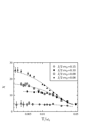
FIG. 1.: Low-temperature behavior of the impurity magnetic susceptibility at $g_{c}=1/4$ and various values of the coupling constant $J$. Notice the semi-logarithmic scales. Dashed curves represent guides to the eye only. Vertical bars give standard deviation error bars due to the MC sampling.

For the results presented below, the average sign is $\langle\xi_{p}\rangle\approx 0.1$, but in practice stable simulations can be carried out even for $\langle\xi_{p}\rangle\approx 0.01$ at the expense of long central processing unit (CPU) times. The Monte Carlo trajectory was drawn from the standard Metropolis algorithm.[22] We have used local updates of the phase fields at $x=0$, i.e., of the Matsubara components $q_{c}(\omega_{n})$ and $q_{s}(\omega_{n})$ for $|\omega_{n}|\leq\omega_{c}$, and of the impurity spin trajectory $S_{z}(t_{j})=S_{j}/2=\pm 1/2$. Typical discretization parameters [for $J/2\pi v_{F}=0.1$ and $V=0$] required to ensure convergence to the continuum limit of the discretized path integral are $\omega_{c}\delta t\simeq 0.3$. The acceptance ratios for local updates of the $\{S_{j}\}$ variables are rather low for the parameter values considered below, typically of the order of $5\%$. Therefore data are accumulated only after at least $5$ full MC passes to ensure statistical independence. Our code performs at an average speed of 1 CPU hour per $5000$ samples (separated by $5$ MC passes) on an IBM RISC 6000/model 590 workstation at the lowest temperatures under consideration. Results reported here require typically $10^{6}$ samples per data point.

III Critical impurity dynamics without potential scattering

In this section we study the case without potential scattering $(V=0)$, with particular emphasis on the controversy about the low-temperature scaling. From our QMC data we observe that all $\chi(T)$ curves for different coupling constants $J$ but at a given Coulomb interaction strength $g_{c}$ can be mapped onto a single universal scaling curve.

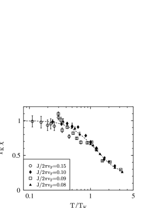
FIG. 2.: Scaling curve for Fig. 1. Notice the semi-logarithmic scales. The dashed curve is a guide to the eye only.

For instance, our raw data for $g_{c}=1/4$ are shown in Fig. 1, and the scaling curve for $\chi$ is depicted in Fig. 2. Apparently, there is a universal scaling function $f$ such that

$$T_{K}\,\chi(T)=f(T/T_{K})\;.$$ (56)

Using this matching procedure, the Kondo temperature can be determined straightforwardly. On the other hand, the value $\chi_{0}=\chi(T=0)$ is finite and can be used to define the Kondo temperature as well. Indeed, the zero-temperature magnetic susceptibility is of the order of the binding energy of the many-body singlet state formed by the impurity spin and the conduction electrons. Therefore we can fix $T_{K}$ alternatively as

$$\chi_{0}=1/T_{K}\;,$$ (57)

which implies $f(0)=1$ from Eq. (56). From the zero-temperature limit of $\chi(T)$ [which can be obtained quite accurately by extrapolation of the data] we can then read off $T_{K}$. By means of either of these two prescriptions, as is shown in Fig. 3 for $g_{c}=1/4$, one can indeed verify the dependence of the Kondo temperature on the coupling constant predicted in Refs. [12] and [13],

$$T_{K}=D\left(\frac{J}{2\pi v_{F}}\right)^{2/(1-g_{c})}\;,$$ (58)

where $D$ is of the order of the bandwidth cutoff $\omega_{c}$. Simultaneously, one gets the universal scaling curve for given interaction strength $g_{c}$.

Now we wish to address the low-temperature critical behavior. The low-temperature form ($T\ll T_{K}$) of the impurity susceptibility (56) can exhibit only two possibilities allowed from conformal field theory (CFT).[14] Either one has (i) Fermi-liquid behavior,

$$f(T/T_{K})=1-c_{1}(T/T_{K})^{2}+\cdots\;,$$ (59)

or (ii) the anomalous exponents predicted by Furusaki and Nagaosa,[13]

$$f(T/T_{K})=1-c_{2}(T/T_{K})^{1/g_{c}}+\cdots\;,$$ (60)

where $c_{1}$ and $c_{2}$ are positive constants. Obviously, at $g_{c}=1/2$ one must see the $T^{2}$ behavior. This is a check for our numerics which is indeed passed nicely. The results (taking $J/2\pi v_{F}=0.1$) are presented in Fig. 4. In the inset we have depicted the dependence of the deviation $(\chi_{0}-\chi)T_{K}$ on the thermal scaling variable $T/T_{K}$. As one can see, the correct $T^{2}$ power law emerges, provided we are below the Kondo temperature.

FIG. 3.: Normalized Kondo temperature $T_{K}$ as a function of the exchange coupling $J$ for $g_{c}=1/4$. The normalization has been chosen such that $T_{K}=1$ for $J/2\pi v_{F}=0.1$. The crosses represent the evaluation of $T_{K}$ from Eq. (56) and the circles from Eq. (57). The straight line has slopand the circles from Eq. (57). The straight line has slope $8/3$ and represents the prediction of Eq. (58). Notice the double-logarithmic scale.

FIG. 4.: Scaling curve for the temperature dependence of the impurity susceptibility at $g_{c}=1/2$. The inset shows the same data for $(\chi_{0}-\chi)T_{K}$ as a function of $T/T_{K}$ at low temperatures again. The straight line in the inset has slope $2$. Notice the double-logarithmic scales. The dotted curve is a guide to the eye only.

The same critical behavior is found for $g_{c}=1/4$ as shown in Fig. 5. At low temperatures, the universal scaling curve displays a $T^{2}$ behavior. The data shown here were obtained for $J/2\pi v_{F}=0.1$, but by virtue of scaling the same curve is found for other $J$ as well. From these results one might be tempted to infer Fermi-liquid behavior for all interaction strength parameters $g_{c}$. However, we find the Furusaki-Nagaosa $T^{1/g_{c}}$ law as soon as $g_{c}>1/2$, as shown in Fig. 6 for $g_{c}=3/4$. The slope in the inset of Fig. 6 is $4/3$, in accordance with the exponent found in Ref. [13].

FIG. 5.: Same as in Fig. 4 but for $g_{c}=1/4$. The straight line in the inset has slope 2.

FIG. 6.: Scaling curve as in Fig. 4 but for $g_{c}=3/4$. The straight line in the inset has slope $4/3$.

In addition, we have analyzed the case of extremely strong interactions. This formally corresponds to $g_{c}\to 0$. Assuming that this limit is analytical, we can find the impurity susceptibility behavior from a study of $g_{c}=0.001$, see Fig. 7. Again, in accordance with our previous analysis, we find a $T^{2}$ law for the low-temperature susceptibility.

FIG. 7.: Scaling curve as in Fig. 4 but for $g_{c}=0.001$. The straight line in the inset has slope $2$.

Let us now discuss these numerical results. Our simulation data for the impurity susceptibility at $T\ll T_{K}$ obey the scaling form (56) with

$$f(T/T_{K})=1-c_{1}(T/T_{K})^{2}-c_{2}(T/T_{K})^{1/g_{c}}+\cdots\;.$$ (61)

Hence there are two leading irrelevant scaling fields,[31] one describing Fermi liquid ($\lambda_{1}$) and one describing non-Fermi liquid ($\lambda_{2}$) behavior, where the latter one corresponds to the Furusaki-Nagaosa prediction. For $g_{c}<1/2$, the Fermi-liquid term is more important and leads to the observed $T^{2}$ behavior at low temperatures. In contrast, for $1/2<g_{c}<1$, the non-Fermi liquid behavior predicted in Ref.[13] dominates.

The scaling form (61) is consistent with the conformal-field theory analysis.[14, 32] The operator $\widehat{O}_{2}$ conjugate to the scaling field $\lambda_{2}$ is produced by a composite boundary operator in spin and charge sectors, while the operator $\widehat{O}_{1}$ comes from a composite operator given by the products of energy-momenta tensors in spin and charge sectors. As these are descendants of the identity operator, their contribution to the susceptibility becomes linear in $\lambda_{1}$, i.e., $c_{1}\sim\lambda_{1}$. In contrast, the Furusaki-Nagaosa term scaling like $T^{1/g_{c}}$ is quadratic in the corresponding scaling field, $c_{2}\sim\lambda^{2}_{2}$. The amplitude of this contribution vanishes $\sim(1-g_{c})$ as $g_{c}\to 1$, thereby reproducing the correct Fermi-liquid behavior of the conventional Kondo effect for uncorrelated electrons. Parenthetically, we note that the scaling field $\lambda_{2}$ also produces a subleading $T^{1+1/g_{c}}$ law in the impurity specific heat.

To summarize, at $g_{c}<1/2$, the Fermi liquid behavior will always dominate. However, at sufficiently low temperatures, the Furusaki-Nagaosa exponents can be observed at $1/2<g_{c}<1$. This finding is in conflict with the recent numerical DMRG study by Wang,[16] which reports Fermi-liquid behavior for a spin-$\frac{1}{2}$ impurity coupled to a Hubbard chain. Notice that the interaction parameter $g_{c}$ for the 1D Hubbard model away from half-filling is always within the bounds $1/2<g_{c}<1$.[6] Most likely the discrepancy is caused by finite-size effects due to the short chain lengths used in Ref. [16]. The more complicated outcome (61) also shows that the simplified model by Schiller and Ingersent[15] does not capture all essentials of the Kondo effect in a Luttinger liquid.

Finally, let us discuss our data for extremely strong interactions, $g_{c}\to 0$. For the clean case, it is well established that the Luttinger liquid model for $g_{c}\to 0$ is equivalent to the low-energy sector of the 1D Heisenberg spin chain.[6] Assuming that this reasoning carries over if a magnetic impurity is present, the $T^{2}$ scaling of the impurity susceptibility observed here (see Fig. 7 for $g_{c}=0.001$) should also describe the susceptibility of a spin-$\frac{1}{2}$ impurity interacting with a 1D Heisenberg chain. One has to be careful to couple the impurity to just one site of the Heisenberg chain, otherwise an additional potential scattering contribution will be present (see Refs.[33, 34, 35, 36] and Sec. IV). A different result was reported very recently by Liu,[37] namely a $T^{5/2}$ scaling of the impurity susceptibility at low temperatures. Unfortunately, the reason for this discrepancy is not clear at the moment.

IV Critical impurity dynamics with potential scattering

In this section the influence of elastic potential scattering on the critical properties of a spin-$\frac{1}{2}$ impurity in a Luttinger liquid will be discussed. As already mentioned in the Introduction, for sufficiently strong interaction strength, $g_{c}<1/2$, and for strong enough potential scattering, the system is expected to display physics familiar from the two-channel Kondo model.[21]

In Fig. 8, data are shown for $g_{c}=1/4$. At high temperatures, with or without elastic potential scattering, the Curie susceptibility of a free spin is always approached,

$$\chi_{\rm free}(T)=\beta/4\;.$$ (62)

However, while the impurity susceptibility displays a crossover to the finite value $\chi_{0}=1/T_{K}$ at zero temperature for vanishing elastic potential scattering strength ($V=0$), the behavior is drastically different if potential scattering is present (here, $2V/\pi v_{F}=0.2$). The impurity susceptibility does not saturate but continues to increase without bound when lowering the temperature. Since we have semi-logarithmic scales in Fig. 8, our data are accurately fitted by the susceptibility of the two-channel Kondo model,[29]

$$\chi(T)\simeq\frac{1}{\pi\Gamma}\ln\left(\frac{\Gamma}{T}\right)\;,$$ (63)

where $\Gamma=J^{2}/2\pi^{2}v_{F}^{2}$. This value for $\Gamma$ (see Ref.[29]) is indeed obtained from the slope of the solid line in Fig. 8.

FIG. 8.: Impurity susceptibility at $g_{c}=1/4$ in the presence of elastic potential scattering, $2V/\pi v_{F}=0.2$, for exchange coupling $J/2\pi v_{F}=0.08$. The data points are given as filled diamonds. For comparison, the $V=0$ data from Fig. 5 are shown as open circles. The solid line has slope $1/\pi\Gamma$ (see text), and the dotted curve gives has slope $1/\pi\Gamma$ (see text), and the dotted curve gives the susceptibility (62) of a free spin. The dashed curve is a guide to the eye only, and $T_{K}$ is computed for $V=0$. Notice the semi-logarithmic scales.

The corresponding results for $g_{c}=3/4$ are shown in Fig. 9. The logarithmically divergent behavior in the presence of potential scattering is not found anymore, and the low-temperature impurity susceptibility saturates at a finite value $\chi^{V}_{0}$. Since $\chi_{0}^{V}>\chi_{0}$, we expect from Eq. (57) that all effects of potential scattering can be incorporated by a renormalization of the Kondo temperature $T_{K}$ to smaller values. Within statistical error bars, the data for $2V/\pi v_{F}=0.3$ shown in Fig. 9 can indeed be scaled onto the $V=0$ data, and the scaling function $f$ holds even in the presence of elastic potential scattering. Clearly, this finding is in sharp contrast to the case of strong interactions, $g_{c}=1/4$, where potential scattering drastically changes the temperature dependence of the impurity susceptibility.

From these data and the arguments of Ref.[21], we then expect two-channel Kondo behavior and hence a logarithmically divergent susceptibility for all $g_{c}<1/2$. An important special case of this general result is recovered for $g_{c}\to 0$ which corresponds to the 1D Heisenberg chain. Using numerical methods, bosonization and CFT techniques, Eggert and Affleck[33] and Clarke et al.[34] have shown that a spin-$\frac{1}{2}$ impurity in a Heisenberg chain exhibits a logarithmically divergent impurity susceptibility. Due to the specific coupling of the impurity to the 1D spin chain in these studies, an additional elastic potential scattering was present besides the usual Kondo exchange coupling term.

FIG. 9.: Impurity susceptibility at $g_{c}=3/4$ in the presence of elastic potential scattering, $2V/\pi v_{F}=0.3$, for exchange coupling $J/2\pi v_{F}=0.1$. Data points are given as filled diamonds. For comparison, the $V=0$ data from Fig. 6 are shown as open circles. The dotted curve gives the susceptibility (62) of a free spin. The dashed curves are guides to the eye only, and $T_{K}$ is computed for $V=0$. Notice the semi-logarithmic scales.

V Conclusions

In this paper the critical behavior of a spin-$\frac{1}{2}$ impurity in a correlated one-dimensional metal (Luttinger liquid) has been investigated numerically. To circumvent finite-size restrictions, we have developed and applied a quantum Monte Carlo algorithm which allows to determine any finite-temperature equilibrium quantity of interest. Here we have focused on the impurity susceptibility $\chi$ with particular emphasis on the low-temperature behavior well below the Kondo temperature. Let us briefly summarize the main findings emerging from our numerically exact analysis.

If elastic potential scattering is ignored, the impurity susceptibility shows the scaling behavior $T_{K}\chi(T)=f(T/T_{K})$ with a distinct universal scaling function $f$ for each dimensionless interaction strength $g_{c}$. It may be worth mentioning that scaling holds even outside the asymptotic low-temperature regime $T\ll T_{K}$. Within error bars, all data can be scaled onto universal scaling functions as long as $T\ll\omega_{c}$, where $\omega_{c}$ is the bandwidth. Matching $\chi(T)$ curves for different $J$ (but at a given $g_{c}$) onto a scaling curve also yields the correct power-law dependence of the Kondo temperature, $T_{K}\sim J^{2/(1-g_{c})}$, which was first given in Ref.[12].

We have then used our algorithm to determine the critical behavior for $T\ll T_{K}$. Generally one finds power laws $\chi(T)\sim(T/T_{K})^{\eta}$ with some exponent $\eta$. At $g_{c}=1/4$ and $g_{c}=1/2$, we find $\eta=2$, but at $g_{c}=3/4$, a different exponent $\eta=4/3$ is obtained. Our data are consistent with the simultaneous existence of two leading irrelevant operators, one describing Fermi-liquid behavior ($\eta=2$), the other describing the Furusaki-Nagaosa[13] anomalous exponent $\eta=1/g_{c}$. At $g_{c}<1/2$, the Fermi-liquid behavior is dominant, but at $1/2<g_{c}<1$, one can indeed observe the $g_{c}$-dependent exponents. These findings resolve the recent controversy[14, 15, 16, 17, 18] about the low-temperature criticality of the Kondo effect in a Luttinger liquid.

We have also studied the effects of elastic potential scattering using our numerical approach. As predicted by Fabrizio and Gogolin,[21] for sufficiently strong Coulomb interaction strength, $g_{c}<1/2$, the impurity susceptibility exhibits a logarithmically divergent behavior. The $\chi\sim\ln(1/T)$ scaling is a manifestation of two-channel Kondo physics caused by the effectively open boundary at the impurity site. In contrast, for $1/2<g_{c}<1$, the susceptibility saturates to a finite value at zero temperature and potential scattering does not modify the critical behavior.

To conclude, we have numerically examined the critical scaling properties of the Kondo effect in a Luttinger liquid. An interesting question which has not yet been studied in detail is related to universality in the presence of potential scattering, e.g., the existence of universal scaling functions for the impurity susceptibility. Future applications of our Monte Carlo algorithm might also deal with the case of more than one impurity, or with a systematic study of other quantities like the impurity specific heat.

- [1] J. Kondo, Progr. Theor. Phys. 32, 37 (1964).
- [2] A.C. Hewson, The Kondo Problem to Heavy Fermions (Cambridge University Press, Cambridge, 1993).
- [3] P. Nozières, J. Low. Temp. Phys. 17, 31 (1974).
- [4] F.D.M. Haldane, J. Phys. C 14, 2585 (1981).
- [5] J. Voit, Rep. Progr. Phys. 58, 977 (1995).
- [6] H.J. Schulz, in Mesoscopic Quantum Physics, Les Houches Session LXI, edited by E. Akkermans, G. Montambaux, J.L. Pichard, and J. Zinn-Justin (Elsevier, 1995).
- [7] S. Tarucha, T. Honda, and T. Saku, Solid State Comm. 94, 413 (1995); A. Yacoby, H.L. Stormer, N.S. Wingreen, L.N. Pfeiffer, K.W. Baldwin, and K.W. West, Phys. Rev. Lett. 77, 4612 (1996).
- [8] J.M. Calleja, A.F. Goñi, B.S Dennis, J.S. Weiner, A. Pinczuk, S. Schmitt-Rink, L.N. Pfeiffer, K.W. West, J.F. Müller, and A.E. Ruckenstein, Solid State Commun. 79, 911 (1991).
- [9] S. Iijima, Nature 354, 56 (1991); S.J. Tans, M.H. Devoret, H. Dai, A. Thess, R.E. Smalley, L.J. Geerligs, and C. Dekker, ibid. 386, 474 (1997).
- [10] A.M. Chang, L.N. Pfeiffer, and K.W. West, Phys. Rev. Lett. 77, 2538 (1996).
- [11] See, e.g., C.L. Kane and M.P.A. Fisher, Phys. Rev. B 46, 15 233 (1992); K.A. Matveev, D. Yue, and L.I. Glazman, Phys. Rev. Lett. 71, 3351 (1993); A. Furusaki and N. Nagaosa, Phys. Rev. B 47, 4631 (1993); P. Fendley, A.W.W. Ludwig, and H. Saleur, Phys. Rev. Lett. 74, 3005 (1995); U. Weiss, R. Egger, and M. Sassetti, Phys. Rev. B 52, 16 707 (1995).
- [12] D.H. Lee and J. Toner, Phys. Rev. Lett. 69, 3378 (1992).
- [13] A. Furusaki and N. Nagaosa, Phys. Rev. Lett. 72, 892 (1994).
- [14] P. Fröjdh and H. Johannesson, Phys. Rev. Lett. 75, 300 (1995); Phys. Rev. B 53, 3211 (1996).
- [15] A. Schiller and K. Ingersent, Phys. Rev. B 51, 4676 (1995). See also P. Phillips and N. Sandler, ibid. 53, R468 (1996).
- [16] X. Wang, preprint cond-mat/9705302.
- [17] H. Chen, Y.M. Zhang, Z.B. Su, and Lu Yu, preprint.
- [18] Y. Wang and J. Voit, Phys. Rev. Lett. 77, 4934 (1996).
- [19] K. Hallberg and C. Balseiro, Phys. Rev. B 52, 374 (1995).
- [20] T. Schork and P. Fulde, Phys. Rev. B 50, 1345 (1994); G. Khaliullin and P. Fulde, ibid. 52, 9514 (1995); Y.M. Li, ibid. 52, R6979 (1995).
- [21] M. Fabrizio and A.O. Gogolin, Phys. Rev. B 51, 17 827 (1995).
- [22] Applications of the Monte Carlo method in statistical physics, edited by K. Binder (Springer, 1987).
- [23] E.H. Loh Jr., J.E. Gubernatis, R.T. Scalettar, S.R. White, D.J. Scalapino, and R.L. Sugar, Phys. Rev. B 41, 9301 (1990).
- [24] C.H. Mak, Phys. Rev. Lett. 68, 899 (1992).
- [25] We have also tried to implement the Monte Carlo algorithm using other strategies, e.g., based on the Coulomb gas representation of Ref.[12] or using spin-coherent state path-integral representations of the magnetic impurity [see, e.g., A. Auerbach, Interacting Electrons and Quantum Magnetism (Springer, 1994)]. These other approaches are all plagued by a very significant sign problem and have therefore been abandoned.
- [26] R. Egger and H. Schoeller, Phys. Rev. B 54, 16 337 (1996).
- [27] J. Hirsch and R.M. Fye, Phys. Rev. Lett. 56, 2521 (1986).
- [28] K.D. Schotte and U. Schotte, Phys. Rev. B 4, 2228 (1971).
- [29] V.J. Emery and S. Kivelson, Phys. Rev. B 46, 10 812 (1992); Phys. Rev. Lett. 71, 3701 (1993).
- [30] R. Egger and H. Grabert, Phys. Rev. Lett. 75, 3505 (1995).
- [31] J. Cardy, Scaling and Renormalization in Statistical Physics (Cambridge University Press, Cambridge, 1996).
- [32] M. Granath and H. Johannesson, unpublished.
- [33] S. Eggert and I. Affleck, Phys. Rev. B 46, 10 866 (1992); Phys. Rev. Lett. 75, 934 (1995).
- [34] D.G. Clarke, T. Giamarchi and B.I. Shraiman, Phys. Rev. B 48, 7070 (1993).
- [35] W. Zhang, J. Igarashi, and P. Fulde, Phys. Rev. B 54, 15 171 (1996); ibid. 56, 654 (1997).
- [36] A.A. Zvyagin and P. Schlottmann, Phys. Rev. B 56, 300 (1997).
- [37] Y.L. Liu, Phys. Rev. Lett. 79, 293 (1997).