Fluctuation Conductivity in Mesoscopic Superconductor - Normal Metal Contacts

Abstract

The fluctuation Conduction of NSN and SNS contacts above $T_{c}$ are analyzed. For NSN contacts, both Aslamazov - Larkin and Maki - Thompson corrections to the conduction are found to be of the same order and diverge for $T_{c}^{*}<T_{c}$ according to the law $(T-T_{c}^{*})^{-1}$. For SNS contacts, the Aslamazov - Larkin correction vanishes, while the Maki - Thompson correction is essential for contacts shorter than the phase-breaking length.

Pacs numbers: 72.10Bg, 73.40Gk, 74.50.+r

I INTRODUCTION

Recently, mesoscopic superconducting - normal metal(S/N) systems have attracted a great deal of attention [1] - [7]. In particular, it was shown that their conductance exhibits oscillatory behavior in magnetic field [1] - [5] and nonmonotonic temperature and voltage dependences [5]. The reason for this behaviour is the effect superconducting correlations have on the electrons in the normal metal. The physics of these effects is simillar to the physics of corrections to the conductivity resulting from superconducting fluctuations above $T_{c}$ [14], [15], [16]. In particular, the authors of ref [8] have shown that the nonmonotonic temperature dependence of conductance in S/N systems is the result of competition between the contribution from the modified density of states and a contribution which is similar to the Maki - Thompson (MT) fluctuation conductivity above $T_{c}$ [15], [16]. Therefore, it is of interest to calculate the conductance of different S/N systems above $T_{c}$ taking into account superconducting fluctuations.

Despite the large number of papers concerned with superconducting fluctuations in macroscopic samples, very few authors have considered superconducting fluctuations in contacts. In particular, Kulik [9] considered the effect of superconducting fluctuations on the density of states and on the current in a tunnel junction. Zaitsev [10] considered the fluctuation corrections to the conductance of very short superconducting microbridges. However, these studies have revealed only two types of fluctuation corrections in uniform systems; the correction due to the modified density of states and the MT correction, which represents the effect of fluctuational Cooper pairs on the conduction of normal electrons. They did not reveal the Aslamazov - Larkin (AL) correction [14] which represents the direct contribution of fluctuational Cooper pairs to the current.

In this paper, we consider the effects of superconducting fluctuations on the conductance of mesoscopic NSN and SNS contacts of various lengths. In the case of NSN contacts, we find that the AL and MT corrections are of the same order of magnitude. In the case of SNS contacts, the conductance is determined by the MT correction, which penetrates into the contact, from the electrodes, a distance upto the phase-breaking length $L_{\varphi}$.

II BASIC EQUATIONS

The expressions determining the superconducting corrections to the conductivity are easily obtained by a trivial extension of the Aslamazov - Larkin and Maki - Thompson equations to inhomogeneous systems. However, as many people are not familiar with the diagrammatic technique used by these authors, we present here a different derivation based on quasiclassical Green’s functions of the superconductor and the self-consistency equation with a Langevin source [11],[10], [12]. One can show that the results obtained with the aid of the diagrammatic technique and the results presented here are identical.

The current density in a dirty superconductor is expressed by the formula

$${\bf j}=\frac{\pi}{2}eN_{F}D\int\frac{d\epsilon}{2\pi}\int\frac{d\epsilon^{\prime}}{2\pi}\,{\rm Sp}\left\{\hat{\tau}_{z}\left[\hat{g}^{R}(\epsilon,\epsilon^{\prime})\frac{\partial\hat{g}^{F}(\epsilon,\epsilon^{\prime})}{\partial\bf r}-\hat{g}^{F}(\epsilon,\epsilon^{\prime})\frac{\partial\hat{g}^{A}(\epsilon,\epsilon^{\prime})}{\partial\bf r}\right]\right\},$$ (1)

where $\hat{g}^{R}$, $\hat{g}^{A}$, and $\hat{g}^{F}$ are quasiclassical matrix Green’s functions of the superconductor [13], $N_{F}=mp_{0}/2\pi^{2}$ is the density of states at the Fermi level, and $D=lv_{0}/3$ is the diffusion coefficient of electrons. The retarded and advanced Green’s functions $\hat{g}^{R(A)}$ describe the energy spectrum of the superconductor, while $\hat{g}^{F}$ also contains information about the electron distribution. In the case of a time-independent electrical potential, the functions $\hat{g}^{R(A)}(\epsilon,\epsilon^{\prime},{\bf r})$ obey the equation

$$-D\frac{\partial}{\partial\bf r}\left(\hat{g}^{R(A)}\frac{\partial\hat{g}^{R(A)}}{\partial\bf r}\right)+\left(-i\epsilon\hat{\tau}_{z}-i\hat{\Delta}+\hat{\Sigma}_{d}^{R(A)}\right)\hat{g}^{R(A)}-\hat{g}^{R(A)}\left(-i\epsilon^{\prime}\hat{\tau}_{z}-i\hat{\Delta}+\hat{\Sigma}_{d}^{R(A)}\right)=0$$ (2)

where

$$\hat{\Delta}=\left(\begin{array}[]{ccc}0&&\Delta\\ -\Delta^{*}&&0\\ \end{array}\right),$$

and the matrix $\hat{\Sigma}_{d}^{R(A)}=\pm\Gamma\hat{\tau}_{z}$ describes the depairing. The products of the matrix quantities also imply convolutions over the inner frequencies.

The order parameter $\Delta(\omega,{\bf r})$ satisfies the self-consistency equation containing the source of condensate fluctuations [11]:

$$\Delta(\omega,{\bf r})=\frac{\lambda}{8}\int\frac{d\epsilon}{2\pi}{\rm Sp}\left[(\hat{\tau}_{x}-\hat{\tau}_{y})\hat{g}^{F}(\epsilon+\omega/2,\epsilon-\omega/2,{\bf r})\right]-\lambda\eta(\omega,{\bf r}),$$ (3)

and the correlation function of the sources of fluctuations $\eta$ is given by

$$<\eta(\omega,{\bf r})\eta^{*}(\omega^{\prime},{\bf r^{\prime}})>=(16\pi N_{F})^{-1}\delta(\omega+\omega^{\prime})\delta({\bf r-r^{\prime}})$$ (4)

$$<\eta(\omega,{\bf r})\eta(\omega^{\prime},{\bf r^{\prime}})>=0.$$ (5)

This expression implies that the sources of condenstate fluctuations are $\delta-$ correlated in time. The latter equality is the result of randomness in the phase of superconducting fluctuations above $T_{c}$.

Since the fluctuations of the order parameter are small, the retarded and advanced Green’s functions of the superconductor may be represented as the sum of corresponding normal-metal Green’s functions and a small additive proportional to $\Delta$:

$$\hat{g}^{R(A)}(\epsilon,\epsilon^{\prime})=\pm 2\pi\hat{\tau}_{z}\delta(\epsilon-\epsilon^{\prime})+\hat{f}^{R(A)}(\epsilon,\epsilon^{\prime}).$$ (6)

Substituting Eqn. (6) into Eqn. (2) and making use of the orthogonality condition $[\hat{g}^{R(A)}]^{2}=\hat{1}$ [13], one obtains that

$$\hat{f}^{R(A)}(\epsilon,\epsilon^{\prime},{\bf r})=\pm\int d^{3}{\bf r^{\prime}}\,P^{R(A)}(\epsilon+\epsilon^{\prime},{\bf r},{\bf r^{\prime}})\,\hat{\Delta}(\epsilon-\epsilon^{\prime},{\bf r^{\prime}}),$$ (7)

where the kernels $P^{R(A)}$ are determined by the equations

$$\left(D\partial^{2}/\partial{\bf r}^{2}+i\epsilon-\Gamma\right)P^{R}(\epsilon,{\bf r},{\bf r^{\prime}})=2i\delta({\bf r-r^{\prime}})$$ (8)

$$P^{A}(\epsilon,{\bf r},{\bf r^{\prime}})=-P^{R}(-\epsilon,{\bf r},{\bf r^{\prime}}).$$ (9)

Note that the $\hat{f}^{R(A)}$ matrices contain no diagonal components. The correction to the diagonal components, which determines the density of states, is proportional to the order parameter squared. However, this correction is small for the case under consideration and will be neglected by us.

As the local electron distribution is assumed to be equilibrium, the function $\hat{g}^{F}$ may be expressed in terms of $\hat{g}^{R}$ and $\hat{g}^{A}$ via the relationship

$$\hat{g}^{F}(\epsilon,\epsilon^{\prime})=\hat{g}^{R}(\epsilon,\epsilon^{\prime})\,\hat{n}(\epsilon^{\prime})-\hat{n}(\epsilon)\hat{g}^{A}(\epsilon,\epsilon^{\prime}),$$ (10)

where

$$\hat{n}(\epsilon,{\bf r})=\left(\begin{array}[]{cc}n(\epsilon-e\phi({\bf r}))&0\\ 0&n(\epsilon+e\phi({\bf r}))\\ \end{array}\right),$$

$$n(\epsilon)=\tanh(\epsilon/2T).$$ (11)

and $\phi({\bf r})$ is the electric potential. Substituting Eqns. (10), (7), and (6) into the self-consistency equation (3) gives

$$\Delta(\omega,{\bf r})=\frac{\lambda}{4}\int d^{3}{\bf r^{\prime}}\int\frac{d\epsilon}{2\pi}\Bigl{[}P^{R}(2\epsilon,{\bf r},{\bf r^{\prime}}) n(\epsilon-\omega/2+e\phi({\bf r}))$$ (12)

$$+ P^{A}(2\epsilon,{\bf r},{\bf r^{\prime}})n(\epsilon+\omega/2-e\phi({\bf r}))\Bigr{]}\Delta(\omega,{\bf r^{\prime}})-\lambda\eta(\omega,{\bf r}).$$ (13)

Consider the case where all the relevant length scales are much larger than the characteristic length $\xi_{0}\sim(D/T_{c})^{1/2}$ and $\omega\ll T_{c}$. Then $\Delta({\bf r^{\prime}})$ may be expanded in powers of ${\bf r-r^{\prime}}$ to quadratic terms. Substituting the expression for $P^{R(A)}$ in infinite space,

$$P_{0}^{R(A)}(2\epsilon,{\bf r-r^{\prime}})=\int\frac{d^{3}q}{(2\pi)^{3}}\,\frac{\exp[i{\bf q}({\bf r-r^{\prime}})]}{\epsilon\pm i(Dq^{2}+\Gamma)/2},$$ (14)

into the self-consistency equation (13), one obtains the nonstationary Ginzburg - Landau - Langevin equation in the form

$$\left(D\frac{\partial^{2}}{\partial{\bf r}^{2}}+i\omega-2ie\phi({\bf r})-\tau T_{c}-\Gamma\right)\Delta(\omega,{\bf r})=16T\eta(\omega,{\bf r}),$$ (15)

where $T_{c}$ is the BCS transition temperature and $\tau=(8/\pi)(T-T_{c})/T_{c}$. This equation is well known in the theory of superconducting fluctuations.

Consider now the expression for the current (1). Substituting Eqns. (6) and (10), one obtains:

$${\bf j}={\bf j}_{n}+{\bf j}_{AL}+{\bf j}_{MT},$$ (16)

where

$${\bf j}_{n}=\frac{1}{2}N_{F}De\int d\epsilon\,{\rm Sp}\left(\hat{\tau}_{z}\frac{\partial\hat{n}}{\partial{\bf r}}\right)=\sigma_{n}{\bf E};$$ (17)

$\sigma_{n}$ represents the normal-state conduction. The second term represents the regular Aslamazov - Larkin (AL) correction

$${\bf j}_{AL}=\frac{\pi}{2}eN_{F}D\int\frac{d\epsilon}{2\pi}\int\frac{d\epsilon^{\prime}}{2\pi}\,{\rm Sp}\biggl{\{}\hat{\tau}_{z}\biggl{[}\hat{f}^{R}(\epsilon,\epsilon^{\prime})\frac{\partial\hat{f}^{R}(\epsilon^{\prime},\epsilon)}{\partial{\bf r}}\hat{n}(\epsilon)-\hat{n}(\epsilon)\hat{f}^{A}(\epsilon,\epsilon^{\prime})\frac{\partial\hat{f}^{A}(\epsilon^{\prime},\epsilon)}{\partial{\bf r}}\biggr{]}\biggr{\}}$$ (18)

and the third term represents the anomalous Maki - Thompson (MT) correction

$${\bf j}_{MT}=-\frac{\pi}{2}eN_{F}D\int\frac{d\epsilon}{2\pi}\int\frac{d\epsilon^{\prime}}{2\pi}\,{\rm Sp}\left[\hat{\tau}_{z}\hat{f}^{R}(\epsilon,\epsilon^{\prime})\frac{\partial\hat{n}(\epsilon^{\prime})}{\partial{\bf r}}\hat{f}^{A}(\epsilon^{\prime},\epsilon)\right].$$ (19)

First consider the AL correction. Substituting Eqn. (7) into Eqn. (18) and performing the averaging over the fluctuations of the order parameter, one obtains

$${\bf j}_{AL}=\frac{\pi}{2}eN_{F}D\int\frac{d\epsilon}{2\pi}\int\frac{d\omega}{2\pi}\int d^{3}r_{1}\int d^{3}r_{2}\biggl{[}P^{R}(2\epsilon-\omega,{\bf r},{\bf r}_{1})\frac{\partial P^{R}(2\epsilon-\omega,{\bf r},{\bf r}_{2})}{\partial\bf r}$$

$$-P^{A}(2\epsilon-\omega,{\bf r},{\bf r}_{1})\frac{\partial P^{A}(2\epsilon-\omega,{\bf r},{\bf r}_{2})}{\partial\bf r}\biggr{]}\bigl{[}<\Delta^{*}(\omega,{\bf r}_{1})\Delta(-\omega,{\bf r}_{2})>n(\epsilon+e\phi)$$

$$-<\Delta(\omega,{\bf r}_{1})\Delta^{*}(-\omega,{\bf r}_{2})>n(\epsilon-e\phi)\bigr{]}.$$ (20)

Equation (20) may be simplified, when the characteristic length scales are much larger than $\xi_{0}$, by setting ${\bf r}_{1}={\bf r}$ in the correlators in second factor of the integrand of (20) and expanding in powers of ${\bf r}_{2}-{\bf r}$ to linear terms. Making use of Eqn. (14) for $P^{R(A)}$ in the infinite space, Eqn. (20) is easily shown to be of the form

$${\bf j}_{AL}({\bf r})=-\frac{i}{4}eN_{F}D\int d\omega\biggr{[}\left<\frac{\partial\Delta(\omega,{\bf r})}{\partial\bf r}\Delta^{*}(-\omega,{\bf r})\right>\left.\frac{\partial n}{\partial\epsilon}\right|_{-\omega/2+e\phi({\bf r})}-\left<\Delta(\omega,{\bf r})\frac{\partial\Delta^{*}(-\omega,{\bf r})}{\partial\bf r}\right>\left.\frac{\partial n}{\partial\epsilon}\right|_{\omega/2-e\phi({\bf r})}\biggl{]}.$$ (21)

This is just the standard Ginzburg - Landau expression for the current. Combined with Eqn. (15), it gives the correction to the current due to fluctuations, which include the effects of a nonlinear electric field.

We now calculate the AL correction to linear terms in the electric field. Using the functions $K^{R}(\omega,{\bf\rho},{\bf\rho^{\prime}})$, the Green’s function of Eqn. (15) with zero potential, and $K^{A}(\omega,{\bf\rho},{\bf\rho^{\prime}})=K^{R}(-\omega,{\bf\rho},{\bf\rho^{\prime}})$, then retaining only linear terms in the electric field, the fluctuation of the order parameter may be written in the form

$$\Delta(\omega,{\bf r})=\int d^{3}{\bf r^{\prime}}\,K^{R}(\omega,{\bf r},{\bf r^{\prime}})\eta(\omega,{\bf r^{\prime}})+2ie\int d^{3}{\bf r^{\prime}}\int d^{3}{\bf r}_{1}\,K^{R}(\omega,{\bf r},{\bf r}_{1})[\phi({\bf r}_{1})-\phi({\bf r})]K^{R}(\omega,{\bf r}_{1},{\bf r^{\prime}})\eta(\omega,{\bf r^{\prime}}),$$

$$\Delta^{*}(-\omega,{\bf r})=\int d^{3}{\bf r^{\prime}}\,K^{A}(\omega,{\bf r},{\bf r^{\prime}})\eta((\omega,{\bf r^{\prime}})-2ie\int d^{3}{\bf r^{\prime}}\int d^{3}{\bf r}_{1}\,K^{A}(\omega,{\bf r},{\bf r}_{1})[\phi({\bf r}_{1})-\phi({\bf r})]K^{A}(\omega,{\bf r}_{1},{\bf r^{\prime}})\eta^{*}(-\omega,{\bf r^{\prime}}).$$ (22)

Note that in comparison with $K^{R}(\omega,{\bf\rho},{\bf\rho^{\prime}})$ defined by Aslamasov and Larkin, this quantity contains an additional factor $mp_{0}/16\pi T_{c}$. Substituting Eqn. (22) and the correlator of the sources of condensate fluctuations Eqn. (5) into Eqn. (21), one obtains the linear AL correction in the form

$${\bf j}_{AL}({\bf r})=\frac{8}{\pi}e^{2}DT\int d\omega\int d^{3}{\bf r}_{1}\int d^{3}{\bf r}_{2}\frac{\partial K^{R}({\bf r},{\bf r}_{1})}{\partial{\bf r}}\bigl{\{}[\phi({\bf r}_{1})-\phi({\bf r})]K^{R}({\bf r}_{1},{\bf r}_{2})$$

$$-[\phi({\bf r}_{2})-\phi({\bf r})]K^{A}({\bf r}_{2},{\bf r}_{1})\bigr{\}}K^{A}({\bf r},{\bf r}_{2}).$$ (23)

Note that for the AL correction, the current - field relationship is substantially nonlocal, i.e., the current density at a given point is determined by the electric field in its vicinity, of radius $\xi(T)\sim\sqrt{D/(T-T_{c})}$. This is a consequence of the large size of fluctuational Cooper pairs near $T_{c}$.

Now we proceed to the MT correction. Substituting Eqn. (7) for $\hat{f}_{R(A)}$ into Eqn. (19), one obtains

$${\bf j}_{MT}({\bf r})=-\pi e^{2}N_{F}D\frac{\partial\phi}{\partial\bf r}\int d^{3}r_{1}\int d^{3}r_{2}\int\frac{d\omega}{2\pi}\left<\Delta(\omega,{\bf r}_{1})\Delta^{*}(-\omega,{\bf r}_{2})\right>$$

$$\times\int\frac{d\epsilon}{2\pi}P^{R}(2\epsilon,{\bf r},{\bf r}_{1})P^{A}(2\epsilon,{\bf r},{\bf r}_{2})\frac{\partial}{\partial\epsilon}n(\epsilon-\omega/2+e\phi({\bf r})).$$ (24)

Retaining only the terms linear in the electric field the MT correction is given by the expression

$$\sigma_{MT}({\bf r})=8e^{2}DT\int d^{3}r_{1}\int d^{3}r_{2}\int d^{3}r^{\prime}\int\frac{d\omega}{2\pi}K^{R}(\omega,{\bf r}_{1},{\bf r^{\prime}})K^{A}(\omega,{\bf r}_{2},{\bf r^{\prime}})\int\frac{d\epsilon}{2\pi}P^{R}(2\epsilon,{\bf r},{\bf r}_{1})P^{A}(2\epsilon,{\bf r},{\bf r}_{2})$$ (25)

Unlike the AL correction, the current-field relationship of the MT correction is purely local, as the electric field directly affects normal electrons rather than fluctuational Cooper pairs.

III NSN CONTACT

Consider the NSN contact in the shape of a narrow channel of length $L\gg\xi_{0}$ and cross-sectional area $S$ connecting two massive electrodes. The transverse dimensions of the channel are assumed to be much smaller than $\xi(T)$. Let the $x$ axis be directed along the channel. The normal-state electric potential in the contact is unperturbed by superconducting fluctuations and has the form $\phi=-Vx/L$, where $V$ is the voltage drop across the contact. As the superconducting corrections to the current essentially depend on the distance from the electrodes, the AL and MT corrections (Eqns. (23) , (25)) should be calculated with the unperturbed potential and then averaged over the length of the contact to ensure current conservation.

First consider the AL correction. As the transverse dimensions of the channel are small, all the relevant quantities may be considered to be dependent only on the longitudinal coordinate $x$. Introduce a system of the eigenfuctions of the Laplace equation

$$\varphi_{n}(x)=\sqrt{\frac{2}{L}}\sin\left(\frac{\pi nx}{L}\right).$$ (26)

Then the function $K^{R}$ entering into Eqn. (23), the Green’s function of Eqn. (15) with zero boundary conditions at the ends of the contact, may be represented in the form

$$K^{R}(x,x^{\prime})=-\frac{i}{S}\sum_{n}\frac{\varphi_{n}(x)\varphi_{n}(x^{\prime})}{\omega+i\epsilon_{L}(\pi^{2}n^{2}+\tau_{L}+\gamma)},$$ (27)

where $\epsilon_{L}=D/L^{2}$ is the Thouless energy, $\tau_{L}=\tau T_{c}/\epsilon_{L}$, and $\gamma=\Gamma/\epsilon_{L}$. Performing the integration in Eqn. (23) over the coordinates and frequency and making use of the relationships

$$\int\limits_{0}^{L}dx\,\varphi_{m}(x)x\varphi_{n}(x)\,=\,\left\{\begin{array}[]{cc}-\frac{\displaystyle 4}{\displaystyle\pi^{2}}L\frac{\displaystyle mn}{\displaystyle(m^{2}-n^{2})^{2}}\bigr{[}1-(-1)^{m+n}\bigl{]},&m\neq n\\ &\\ L/2,&m=n,\end{array}\right.$$ (28)

$$\int\limits_{0}^{L}dx\,\frac{\partial\varphi_{m}}{\partial x}\varphi_{n}(x)=\left\{\begin{array}[]{cc}-\frac{\displaystyle 2}{\displaystyle L}\frac{\displaystyle mn}{\displaystyle n^{2}-m^{2}}\bigr{[}1-(-1)^{m+n}\bigl{]},&m\neq n\\ &\\ 0,&m=n,\end{array}\right.$$ (29)

one obtains the AL correction in the form

$$\delta I_{AL}=64\frac{e^{2}TV}{\epsilon_{L}}\sum_{m}\sum_{n\neq m}\left(\frac{mn}{m^{2}-n^{2}}\right)^{2}\frac{\bigl{[}1-(-1)^{m+n}\bigr{]}^{2}}{\theta_{m}\theta_{n}(\theta_{m}+\theta_{n})},$$ (30)

where $\theta_{m}=\pi^{2}m^{2}+\tau_{L}+\gamma$. In the limit $\tau_{L}\gg 1\gg\gamma$, Eqn. (30) gives the standard AL correction for the one-dimensional wire

$$\delta I_{AL}=\frac{\pi^{3/2}}{2^{11/2}}\frac{e^{2}T\epsilon_{L}^{1/2}}{(T-T_{c})^{3/2}}V.$$ (31)

The AL correction (30) remains finite at $T=T_{c}$ owing to the finite length of the contact, the transition temperature decreases from the bulk value to the value

$$T_{c}^{*}=T_{c}-\frac{\pi}{8}\Gamma-\frac{\pi^{3}}{8}\epsilon_{L}.$$ (32)

Near $T_{c}^{*}$ the temperature dependence of AL correction is of the form

$$\delta I_{AL}=a\frac{e^{2}TV}{T-T_{c}^{*}},$$

$$a=\frac{1}{\pi^{3}}\sum_{k=1}^{\infty}\frac{k^{2}}{(k^{2}-1)^{4}}\approx 0.1026.$$ (33)

Now we proceed to the MT correction. As the quantities $P^{R(A)}$ appearing in Eqn. (25) also satisfy the zero boundary conditions at the ends of the contacts, they have the form

$$P^{R}(\epsilon,x,x^{\prime})=\frac{2}{S}\sum_{n}\frac{\varphi_{n}(x)\varphi_{n}(x^{\prime})}{\epsilon+i\epsilon_{L}(\pi^{2}n^{2}+\gamma)}.$$ (34)

Substituting Eqns. (27) and (34) into Eqn. (25), averaging over the contact length and summing the resulting series one obtains

$$\delta I_{MT}=2e^{2}V\frac{1}{\tau}\left\{\frac{1}{\gamma^{1/2}}\left(\coth\gamma^{1/2}-\frac{1}{\gamma^{1/2}}\right)-\frac{1}{(\tau_{L}+\gamma)^{1/2}}\left[\coth(\tau_{L}+\gamma)^{1/2}-\frac{1}{(\tau_{L}+\gamma)^{1/2}}\right]\right\}$$ (35)

for $\tau_{L}+\gamma>0$ and

$$\delta I_{MT}=2e^{2}V\frac{1}{|\tau|}\left\{\frac{1}{|\tau_{L}+\gamma|^{1/2}}\left[\frac{1}{|\tau_{L}+\gamma|^{1/2}}-\cot|\tau_{L}+\gamma|^{1/2}\right]-\frac{1}{\gamma^{1/2}}\left(\coth\gamma^{1/2}-\frac{1}{\gamma^{1/2}}\right)\right\}$$ (36)

for $\tau_{L}+\gamma<0$. Alternatively, Eqns.(35) - (36) can be written in the form

$$\delta I_{MT}=4\frac{e^{2}TV}{\epsilon_{L}}\sum_{m}\frac{1}{\theta_{m}(\theta_{m}-\tau_{L})},$$ (37)

For large contact lengths $\tau_{L}\gg 1$, the MT correction reduces to the standard equation for the one-dimensional wire

$$\delta I_{MT}=\frac{\pi}{4}e^{2}V\frac{1}{\tau}\left(\frac{1}{\gamma^{1/2}}-\frac{1}{\tau_{L}^{1/2}}\right).$$ (38)

As well as the AL correction, the MT correction remains finite at $T=T_{c}$ and diverges at $T=T_{c}^{*}$ according to the same law

$$\delta I_{MT}=\frac{1}{2\pi}\frac{e^{2}TV}{T-T_{c}^{*}}.$$ (39)

In Fig. 1 we plotted the temperature dependences of the MT and AL terms in dimentionless fluctuation conductances $S_{MT}$ and $S_{AL}$ for different values of $\gamma$ (the ratio of the depairing rate $\Gamma$ and the Thouless energy $\epsilon_{L}$); here $S_{MT}=\delta I_{MT}/I_{o}\,,\,S_{AL}=\delta I_{AL}/I_{o}\,,\,I_{o}=e^{2}VT/\epsilon_{L}$. As may be seen from Fig. 1, the MT contribution dominates over the whole temperature range. The depairing rate $\Gamma$ can be determined from measurements of the fluctuation conductance.

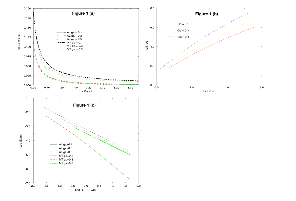
FIG. 1.: Figure 1 (a), shows the MT and the AL terms for several values of $\gamma$ (ga). Figure 1 (b), shows the ration of MT/AL terms for several values of $\gamma$ (ga). Figure 1 (c) is a Log-Log plot of Figure 1 (a).

IV SNS CONTACT

Consider a structure of similar geometry as the structures considered perviously but with a normal-metal channel and superconducting electrodes. The superconductor and normal metal are characterized by the diffusion coefficients $D_{s}$ and $D_{n}$ and by the phase-breaking rates $\Gamma_{s}$ and $\Gamma_{n}$, respectively. In the case of SNS contacts, the fluctuational Cooper pairs generated in the superconducting electrodes can penetrate into the normal metal only a distance shorter than $\xi_{0}$ as the BCS coupling constant $\lambda$ is zero in the normal metal. However, as well as in the superconducting state at $T<T_{c}$ [6], [7], they can affect the conduction of normal electrons at distances much larger than the phase-breaking length $L_{\varphi}$. In this case, the conductance of the contact depends on the geometry of the electrodes even though their dimensions are much larger than the transverse dimensions of the contact.

In view of this reasoning, the AL correction is negligible in SNS contacts. The MT correction is obtained by averaging Eqn. (25) over the contact length, then integrating with respect to ${\bf r}_{1}$, ${\bf r}_{2}$, and ${\bf r^{\prime}}$ over the bulk of both electrodes, each giving an independent contribution to the conductance of the contact. Hence in Eqn. (25), one may use the expressions for $K^{R(A)}$ in a bulk homogeneous superconductor:

$$K^{R}(\omega,{\bf r},{\bf r^{\prime}})=-\frac{i}{\Omega}\sum_{\bf q}\frac{\exp[i{\bf q}({\bf r}-{\bf r^{\prime}})]}{\omega+i[D_{s}q^{2}+\tau T_{c}+\Gamma_{s}]},$$ (40)

where $\Omega$ is the normalization volume.

First consider the contribution from the left electrode. Assume that the origin coincides with the left end of the contact. As in the case of NSN contact, all the quantities inside the channel depend only on the longitudinal coordinate $x$. As the integral (25) is dominated by $|{\bf r}_{1}|$ and $|{\bf r}_{2}|$ of the order of $\xi(T)$, i.e., much larger than the transverse dimensions of the contact, the quantity $P^{R}(\epsilon,x,{\bf r})$, where $x$ is the coordinate of a point inside the contact and $\bf r$ is the coordinate of a point inside the left electrode, may be represented in the form

$$P^{R(A)}(\epsilon,x,{\bf r})=P_{0}^{R(A)}(\epsilon,-{\bf r})\,\psi(\pm\epsilon,x),$$ (41)

where $P_{0}^{R}(\epsilon,-{\bf r})$ is given by Eqn. (14) and function $\psi$ is the solution of the equation

$$D_{n}\frac{d^{2}\psi}{dx^{2}}+(i\epsilon-\Gamma_{n})\psi(\epsilon,x)=0$$

with the boundary conditions $\psi(0)=1$ and $\psi(L)=0$. Explicitly, it is given by the expression

$$\psi(\epsilon,x)=\frac{\sinh[\kappa(1-x/L)]}{\sinh\kappa},\qquad\kappa(\epsilon)=(\gamma_{n}-i\epsilon/\epsilon_{L})^{1/2}.$$ (42)

With these expressions and taking into account contributions from both electrodes, Eqn. (25) takes the form

$$\delta I_{MT}=64e^{2}\epsilon_{L}TLSV\frac{1}{\Omega}\sum_{\bf q}\int\frac{d\omega}{2\pi}\,\frac{1}{\omega^{2}+(D_{s}q^{2}+\tau T_{c}+\Gamma_{s})^{2}}\int\frac{d\epsilon}{2\pi}\,\frac{1}{4\epsilon^{2}+(D_{s}q^{2}+\Gamma_{s})^{2}}\Phi(2\epsilon),$$ (43)

where

$$\Phi(\epsilon)=\frac{1}{L}\int\limits_{0}^{L}dx\,\psi(\epsilon,x)\psi(-\epsilon,x)=\frac{(2\kappa_{1})^{-1}\sinh(2\kappa_{1})-(2\kappa_{2})^{-1}\sin(2\kappa_{2})}{\cosh(2\kappa_{1})-\cos(2\kappa_{2})},$$

$$\kappa_{1}={\rm Re}[\kappa(\epsilon)],\quad\kappa_{2}={\rm Im}[\kappa(\epsilon)].$$ (44)

Integrating with respect to frequency $\omega$ in Eqn. (43) gives

$$\delta I_{MT}=32e^{2}\epsilon_{L}TLSV\frac{1}{\Omega}\sum_{\bf q}\frac{1}{D_{s}q^{2}+\tau T_{c}+\Gamma_{s}}\int\frac{d\epsilon}{2\pi}\,\frac{1}{4\epsilon^{2}+(D_{s}q^{2}+\Gamma_{s})^{2}}\Phi(2\epsilon).$$ (45)

To be specific, consider the case where the electrodes represent a film of thickness $d_{0}<\xi(T)$, then in this case the sum over $\bf q$ may be replaced by the integral

$$\frac{1}{\Omega}\sum_{\bf q}\to\frac{1}{d_{0}}\int\frac{d^{2}q}{(2\pi)^{2}}.$$

Introducing the dimensionless integration variable $\theta=2\epsilon/\epsilon_{L}$, one arrives at the following expression:

$$\delta I_{MT}=\frac{4e^{2}}{\pi^{2}}\frac{TLS}{D_{s}d_{0}}V\int\limits_{0}^{\infty}\frac{d\theta}{\theta^{2}+\tau_{L}^{2}}\left[\ln\left(\frac{\sqrt{\theta^{2}+\gamma_{s}^{2}}}{\tau_{L}+\gamma_{s}}\right)+\frac{\tau_{L}}{\theta}\arctan\left(\frac{\theta}{\gamma_{s}}\right)\right]\frac{\theta_{1}^{-1}\sinh\theta_{1}-\theta_{2}^{-1}\sin\theta_{2}}{\cosh\theta_{1}-\cos\theta_{2}},$$

$$\theta_{1}=2^{1/2}\left(\gamma_{n}+\sqrt{\gamma_{n}^{2}+\theta^{2}}\right)^{1/2},\quad\theta_{2}=2^{1/2}\left(\sqrt{\gamma_{n}^{2}+\theta^{2}}-\gamma_{n}\right)^{1/2}.$$ (46)

Assume for simplicity that the depairing rates in the normal and superconducting metals are equal ($\gamma_{s}=\gamma_{n}=\gamma$). First consider the case of a very short contact, $\gamma\ll\tau_{L}\ll 1$. In this case, the integral (46) is dominated by $\theta\sim\tau_{L}$, so the last factor in the integrand may be set equal to 1/3. This yields

$$\delta I_{MT}=\frac{1}{12}\frac{D_{n}}{D_{s}}\frac{e^{2}}{d_{0}\tau}\ln\left(1+\frac{\tau T_{c}}{\Gamma}\right)\frac{SV}{L}.$$ (47)

To within the factor $D_{n}/D_{s}$ and a numerical coefficient, the correction to the conductivity of the contact material is equal to the MT conductivity of the electrodes. A similar result was previously obtained by Zaitsev [10] for short ScS contacts.

Consider now the case where the contact is of intermediate length, $\gamma\ll 1\ll\tau_{L}$, one obtains with logarithmic accuracy

$$\delta I_{MT}=\frac{1}{12}\frac{D_{n}}{D_{s}}\frac{e^{2}}{d_{0}\tau}\ln(1/\gamma)\frac{SV}{L}.$$ (48)

This expression differs from that for the short contact in that the quantity $(8/\pi)(T-T_{c})$ in the logarithm is replaced by the Thouless energy $\epsilon_{L}$.

Lastly, consider the case of a long contact, $1\ll\gamma\ll\tau_{L}$. In that case, the integral (46) is dominated by $\theta\gg 1$, so the second factor in the integrand may be approximated by $(2\theta)^{-1/2}$, yielding

$$\delta I_{MT}=\frac{1}{2}\frac{D_{n}}{D_{s}}\frac{e^{2}}{d_{0}\tau}\gamma^{-1/2}\frac{SV}{L}.$$ (49)

The physical meaning of this result is that the superconducting correlations that result in the MT correction penetrate into the contact over the length $L_{\varphi}\sim\gamma^{-1/2}L\ll L$.

Note that unlike the case of NSN contact, the correction to the total current is proportional to the cross-sectional area of the contact.

V Conclusions

The fluctuation conductivities of NSN and SNS contacts of arbitrary lengths have been calculated. We have established that the fluctuation conductivity in NSN contacts consists of contributions from both the Maki - Thompson and Aslamasov - Larkin terms. The MT contribution dominates over the whole temperature range. However, near the renormalized critical temperature $T_{c}^{*}$ the ratio of the MT and AL terms does not contain any parameters, and equals about 1.56 .

In SNS contacts the AL contribution is absent. The increase in the conductivity due to fluctuations is caused by the anomalous MT term containing the product of retarded and advanced functions (see Eqn. (25)).

The superconducting fluctuations modiify the density of states and decrease the conductivity. In the case of NSN and SNS contacts analyzed by us, this decrease is small (i.e. it does not diverge as $T$ tends to $T_{c}^{*}$). However the correction to the conductivity due to the decrease of the density of states is essential in SNS contacts at $T<T_{c}^{*}$, this leads to the reentrant behaviour of the conductance [6],[7], [8], and is also essential in tunnel SIS junctions [9] and in layered superconductors [12],[17]

VI Acknowledments

This work was supported by the Russian Foundation for Basic Research, grant 96-02-16663-a,the Russian Superconductivity Program, grant no. 96053, the Royal Society, and by the CRDF, grant no. RP1 - 165. We would also like to thank C. J. Lambert for his attention and useful suggestions to this work.

REFERENCES

• [1] V.T. Petrashov, V.N. Antonov, P. Delsing, and T. Claeson, Phys. Rev. Lett. 70, 347 (1993); Phys. Rev. Lett. 74, 5268 (1995).
• [2] H. Pothier, S. Gueron, D. Esteve, and M.H. Devoret, Phys. Rev. Lett. 73, 2488 (1994).
• [3] P.G.N. de Vedgar, T.A. Fulton, W.H. Mallison, and R.E. Miller, Phys. Rev. Lett. 73, 1416 (1994).
• [4] H. Dimoulas, J.P. Heida, B.J. van Wees, T.M. Klapwijk, W. van der Graaf, and G. Borghs, Phys. Rev. Lett. 74, 602 (1992).
• [5] H. Courtois, Ph. Grandit, D. Maily, and B. Pannetier, Phys. Rev. Lett. 76, 130 (1996).
• [6] A.F. Volkov, N. Allsopp, and C.J. Lambert, J. Phys.: Condens. Matter 8, 45 (1996).
• [7] Yu. V. Nazarov and T.H. Stoof, Phys. Rev. Lett. 76, 823 (1996).
• [8] A.F. Volkov and V.P. Pavlovskii, in Correlated Fermions and Transport in Mesoscopic Systems, Proc. XXXI Moriond Conf., Les Arcs, 1996, p. 267.
• [9] I.O. Kulik, Sov. Phys. JETP 32, 510 (1971).
• [10] A. V. Zaitsev, Sov. Phys. Solid State 26, 1619 (1984).
• [11] A.I. Larkin and Yu.N. Ovchinnikov, J. Low Temp. Phys. 10, 407 (1973).
• [12] A.F. Volkov, Phys. Lett. A 175, 445 (1993); Solid State Commun. bf 88, 715 (1993).
• [13] A.I. Larkin and Yu.N. Ovchinnikov, in Nonequilibrium Superconductivity, Eds. D.N. Langenberg and A.I. Larkin, Elsevier, Amsterdam, 1986, p. 493.
• [14] L.G. Aslamazov and A.I. Larkin, Sov. Phys. Solid State 10, 875 (1968).
• [15] K. Maki, Progr. Theor. Phys 39, 897 (1968).
• [16] R.S. Thompson, Phys. Rev. B1, 327 (1970).
• [17] A.I. Larkin, A.Varlamov, and L.Yu, Phys. Rev. B47, 8936 (1993).