The effect of chain stiffness on the phase behaviour of isolated homopolymers

Abstract

We have studied the thermodynamics of isolated homopolymer chains of varying stiffness using a lattice model. A complex phase behaviour is found; phases include chain-folded ‘crystalline’ structures, the disordered globule and the coil. It is found, in agreement with recent theoretical calculations, that the temperature at which the solid-globule transition occurs increases with chain stiffness, whilst the $\theta$-point has only a weak dependence on stiffness. Therefore, for sufficiently stiff chains there is no globular phase and the polymer passes directly from the solid to the coil. This effect is analogous to the disappearance of the liquid phase observed for simple atomic systems as the range of the potential is decreased.

I Introduction

Most of the work on the thermodynamics of isolated homopolymers has concentrated on the collapse transition between the high temperature coil and the lower temperature dense globule. This emphasis is a result of the extensive theoretical work on the transition[1, 2] and the relative ease of simulations at these low densities—indeed simulations have been performed up to very large sizes,[3] thus providing detailed tests of theoretical predictions.

In contrast, there has been much less interest in the possibility of a low temperature order-disorder transition between two dense phases both because of the greater difficulty of simulating dense polymers and because fewer theoretical expectations for such a transition are available. This situation contrasts with that for heteropolymers where, in the context of protein folding, there has been intense interest in the transition between the molten globule and the native state of the protein. The structure of the native state reflects the amino acid sequence and the specific interactions between these units, and so it might be thought that an ordered structure is less likely when all polymer units are identical. However, this is not the lesson from other finite systems. For example, homogeneous atomic clusters show a rich low temperature phase behaviour; there is the finite-size analogue of the first-order melting transition,[4, 5] surface melting,[6] and even low temperature transitions between different ordered forms.[7]

Recently, the existence of an isolated homopolymer order-disorder transition has begun to be confirmed.[8, 9, 10] In their study of a lattice homopolymer model which involved three-body forces Kuznetsov et al. found phases with orientational order,[9] and in their simple off-lattice model Zhou et al. observed a order-disorder transition and also a solid-solid transition.[10] Moreover, in some earlier studies of the collapsed polymer glimpses of these transitions were seen.[11, 12, 13, 14] Here, we add to this growing understanding of the low temperature phase behaviour of isolated homopolymers by studying a lattice model of a semi-flexible polymer, looking particularly at the effect of stiffness on the order-disorder transition. We compare our results with the phase diagram calculated in recent theoretical[15] and simulation[16] studies of the polymer model we use here.

II Methods

A Polymer Model

In our model the polymer is represented by an $N$-unit self-avoiding walk on a simple cubic lattice. There is an attractive energy, $\epsilon$, between non-bonded polymer units on adjacent lattice sites and an energetic penalty, $\epsilon_{g}$, for kinks in the chain. The total energy is given by

$$E=-n_{pp}\epsilon+n_{g}\epsilon_{g}$$ (1)

where $n_{pp}$ is the number of polymer-polymer contacts and $n_{g}$ is the number of kinks or ‘gauche bonds’ in the chain. $\epsilon$ can be considered to be an effective interaction representing the combined effects of polymer-polymer, polymer-solvent and solvent-solvent interactions, and so our model is a simplified representation of a semi-flexible polymer in solution. The behaviour of the polymer is controlled by the ratio $kT/\epsilon$; large values can be considered as either high temperature or good solvent conditions, and low values as low temperature or bad solvent conditions. The parameter $\epsilon_{g}$ defines the stiffness of the chain. The polymer chain is flexible at $\epsilon_{g}$=0 and becomes stiffer as $\epsilon_{g}$ increases. In this study we only consider $\epsilon_{g}\geq 0$.

When $\epsilon_{g}=0$, this model corresponds to one originated by Orr[17] and has been much used to study homopolymer collapse.[3, 14, 18, 19, 20] The system with positive $\epsilon_{g}$ has been recently studied theoretically by Doniach et al.[15] and using simulation by Bastolla and Grassberger.[16] In our work we pay special attention to the structural changes of a polymer of a specific size. In this sense our work is complementary to that of ref. [16] which focussed on the accurate mapping of the phase diagram.

Our model was chosen because we wished to have the simplest model in which we could understand the effects of stiffness, and because it gives low energy states that have chain folds resembling those found in lamellar homopolymer crystals.[21] Similar structures have previously been seen in a diamond-lattice model of semi-flexible polymers,[11, 12, 13] and in molecular dynamics simulations of isolated polyethylene chains.[22, 23, 24] Particular mention should be made of the studies by Kolinski et al. on the effect of chain stiffness on collapse[11, 12, 13] since they found evidence for many of the phenomena that we explore systematically here.

The global minimum at a particular (positive) $\epsilon_{g}$ is determined by a balance between maximizing $n_{pp}$ and minimizing $n_{g}$. If the polymer is able to form a structure that is a cuboid with dimensions $a\times b\times c$ ($N=abc$), where $a\leq b\leq c$, then

$$n_{pp}=2N-ab-ac-bc+1$$ (2)

and

$$n_{g}^{min}=2ab-2$$ (3)

The structures that correspond to $n_{g}=n_{g}^{min}$ have the polymer chain folded back and forth along the longest dimension of the cuboid. By minimizing the resulting expression for the energy one finds that the lowest energy polymer configuration should have

$$a=b\quad\hbox{and}\quad{c\over a}=1+{2\epsilon_{g}\over\epsilon}.$$ (4)

Therefore, at $\epsilon_{g}=0$ the ideal shape is a cube and for positive $\epsilon_{g}$ a cuboid extended in one direction, the aspect ratio of which increases as the chain becomes stiffer. As the ideal aspect ratio of the crystallite is independent of $N$, its squared radius of gyration, $R_{g}^{2}$, will scale as $N^{2/3}$; this scaling is the same as for the disordered collapsed globule.

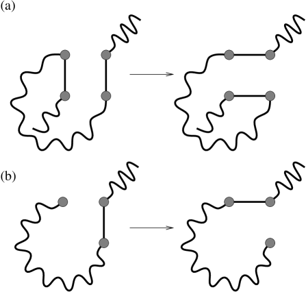
FIG. 1.: Bond-flipping moves. (a) Four-bond flip in which the mid-section of the chain is reordered. Moves of this type were only attempted if they preserved the integrity of the chain. (b) Two-bond flip which results in a new chain end. Only the bonds which change are explicitly depicted; other sections of the polymer are represented by wiggly lines.

Substitution of the optimal dimensions of the cuboid [Equation (4)] into Equations (1)–(3) gives a lower bound to the energy of the global minimum,

$$E_{opt}/\epsilon=-2N+3N^{2/3}(1+2\epsilon_{g}/\epsilon)^{1/3}-1-2\epsilon_{g}/\epsilon.$$ (5)

However, at most sizes and values of $\epsilon_{g}$ it is not possible to form a cuboid with the optimal dimensions, and so the energy of the global minimum will be higher than given by the above expression. Nevertheless, it is easy to find the global minimum just by considering the structures which most closely approximate this ideal shape.

B Simulation Techniques

Recent advances in simulation techniques have made it possible to begin to study dense polymer systems. In particular, we use configurational-bias Monte Carlo[25] including moves in which a mid-section of the chain is regrown.[26] We also make occasional bond-flipping moves [Figure 1] which, although they do not change the shape of the volume occupied by the polymer, change the path of the polymer through that volume.[27, 28] These moves speed up equilibration in the dense phases. The simulation method was tested by comparing to results obtained for $\epsilon_{g}=0$ by exact enumeration.[29, 30] Thermodynamic properties, such as the heat capacity, were calculated from the energy distributions of each run using the multi-histogram method.[31, 32]

The number of Monte Carlo steps used in our simulations was typically 4–30$\times 10^{6}$. The longer simulations were required for the larger polymers, especially at temperatures where two or more states coexisted. The sizes of the polymers we studied were $N$=27, 64, 100, 216, 343. These sizes are ‘magic numbers’ for $\epsilon_{g}=0$, because compact cuboids of low aspect ratios can be formed at these sizes. In the presentation of our results we concentrate on polymers with $N$=100 and 343, the former because the smaller size allows for clear visualization of the structures of the different phases, and the latter because the effects of finite size will be smallest.

TABLE I.: Properties of the global optima for a 100-unit polymer. $\epsilon_{g}^{min}$ and $\epsilon_{g}^{max}$ give the range of $\epsilon_{g}$ for which a structure is the global minimum. $c/\sqrt{ab}$ is the aspect ratio and $\epsilon_{g}^{opt}$ is the value of the stiffness for which a crystallite with that aspect ratio is expected to be lowest in energy and is given by $\epsilon_{g}^{opt}=(c/\sqrt{ab}-1)\epsilon/2$.

	$n_{pp}$	$n_{g}$	$\epsilon_{g}^{min}/\epsilon$	$\epsilon_{g}^{max}/\epsilon$	$c/\sqrt{ab}$	$\epsilon_{g}^{opt}/\epsilon$
A	136	38	0.000	0.375	1.118	0.059
B	133	30	0.375	0.500	1.563	0.281
C	129	22	0.500	0.833	2.406	0.703
D	124	16	0.833	2.167	3.704	1.352
E	111	10	2.167	3.500	6.804	2.902
F	97	6	3.500	12.000	12.500	5.750

In order to monitor the orientational order within the polymer we devised an order parameter, $Q$, which is given by

$$Q={1\over N-1}\sqrt{{3\over 2}\sum_{\alpha=x,y,z}\left(n_{\alpha}-{(N-1)\over 3}\right)^{2}},$$ (6)

where $n_{\alpha}$ is the number of bonds in the direction $\alpha$ and $(N-1)/3$ is the expected value of $n_{\alpha}$ if the bonds are oriented isotropically. $Q$ has a value of 1 if all the bonds are in the same direction, i.e. the polymer has a linear configuration, and a value of 0 if the bonds are oriented isotropically.

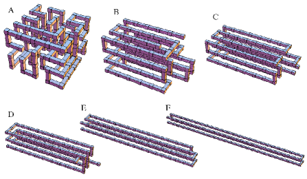
FIG. 2.: Global minima of the 100-unit polymer at different values of $\epsilon_{g}$. The labels correspond to those in Table I.

III Results

A Solid phase

In Table I the properties of the global minima for $N$=100 are given for the range of $\epsilon_{g}$ we consider in this study, and examples of these minima are illustrated in Figure 2. The shapes of the global minima agree well with that expected based on the analysis of section II A. In the final column of Table I we have given the value of the stiffness for which a crystallite with the aspect ratio of the global minimum is expected to be lowest in energy based on Equation (4). This value generally lies in the middle of the range for which the structure is the global minimum. Most of the global minima have a degeneracy associated with the different possible ways of folding the chain back and forth. This degeneracy decreases as the chains become stiffer and the crystallites become more extended. For $\epsilon_{g}=0$ there is no constraint on $n_{g}$, and so the global minimum has a much larger degeneracy, and the majority of the isomers of the global minimum have no orientational order.

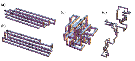
FIG. 3.: Visualizations of various states of a 100-unit polymer. (a) A polymer based on structure D with some disorder in the stem lengths from a simulation at $T=0.9\epsilon k^{-1}$ and $\epsilon_{g}=2\epsilon$. (b) A folded structure with 8 stems that contributes to the middle peak of Figure 5b ($T=1.2\epsilon k^{-1}$, $\epsilon_{g}=3\epsilon$). (c) A typical configuration of the dense globule with $R_{g}^{2}=5.60$ ($T=0.75\epsilon k^{-1}$, $\epsilon_{g}=\epsilon$). (d) A typical configuration of the coil with $R_{g}^{2}=38.91$ ($T=5.0\epsilon k^{-1}$, $\epsilon_{g}=\epsilon$)

The global minimum is the free energy global minimum at zero temperature. However, as the temperature is increased it will become favourable to introduce defects into the structures. One of the mechanisms we commonly observed was through fluctuations in the lengths of the folds, moving in and out like the slide of a trombone. An example of such a structure is shown in Figure 3a. The generation of this type of defect is especially common at larger values of $\epsilon_{g}$ since it does not involve an increase of $n_{g}$.

The dependency of the degeneracy, and therefore the entropy, on the aspect ratio of the crystallites raises the possibility of transitions to crystallites with a smaller aspect ratio as the temperature is increased. Indeed, this is usually what is seen and leads to the decrease of $R_{g}^{2}$ with temperature that is observed before melting [Figure 4]. At the centre of the transition, where the free energy of each crystallite is equal, ideally, the polymer would be seen to oscillate between the two forms [Figure 5a] during the simulation spending equal time in each. This ‘dynamic coexistence’ of structures leads to a bimodal (or even multimodal if more than two forms are stable) distribution of $R_{g}^{2}$ [Figure 5b]. Since the Landau free energy is given by $A_{L}(q)=A-kT\log p_{q}(q)$, where $A$ is the Helmholtz free energy and $p_{q}(q)$ the canonical probability distribution for an order parameter $q$, the multimodality in $R_{g}^{2}$ implies that there are free energy barriers between the different crystallites. In the example shown in Figure 5, the peak with the highest value of $R_{g}^{2}$ corresponds to structures similar to the global minimum D, and the peak with the lowest value of $R_{g}^{2}$ have structures similar to C. The other peak consists of structures that have eight aligned stems, either in a $4\times 2$ array or a square array with one corner unoccupied [Figure 3b].

FIG. 4.: Behaviour of $R_{g}^{2}$ as a function of temperature and $\epsilon_{g}$ for (a) $N$=100 and (b) $N$=343. Each line is labelled by the value of $\epsilon_{g}/\epsilon$.

However, isomerization between the different forms often requires a large-scale change in structure, which is particularly difficult if these transitions occur at low temperature, where the free energy barriers to transitions are largest. With simulation techniques that only apply local moves, transitions between crystallites would be effectively impossible to observe and even with a technique such as configurational-bias Monte Carlo, where global moves are possible, transitions may be rare, particularly for the larger polymers in this study. This possible lack of ergodicity on the simulation time scales can lead occasionally to the abrupt jumps seen in $R_{g}^{2}$ (e.g. for $N$=100 at $\epsilon_{g}$=4$\epsilon$ and $T$=1$\epsilon k^{-1}$, and for $N$=343 at $\epsilon_{g}$=2$\epsilon$ and $T$=0.95$\epsilon k^{-1}$) rather than the smoother transition that would be expected if equilibrium values of $R_{g}^{2}$ were obtained.

FIG. 5.: Solid-solid coexistence observed for a 100-unit polymer with $\epsilon_{g}=3\epsilon$ at $T=1.2\epsilon k^{-1}$. (a) Fluctuations in $R_{g}^{2}$ during a 10 million step Monte Carlo run. (b) Probability distribution of $R_{g}^{2}$.

The differences in energy and entropy between crystallites of different aspect ratio are due to surface effects and so scale less than linearly with size. Therefore, these solid-solid transitions are not finite-size analogues of bulk first-order phase transitions.

Interestingly, this coexistence of polymers with different cuboidal shapes but the same basic structure bears some resemblance to the coexistence of cuboidal sodium chloride clusters that has recently been observed experimentally.[33] All the clusters have the rock-salt structure but the cuboids have different dimensions.

FIG. 6.: Behaviour of (a) $Q$ and (b) $C_{v}$ as a function of temperature and $\epsilon_{g}$ for $N$=343. Each line is labelled by the value of $\epsilon_{g}/\epsilon$.

B Solid-globule/coil transition

For $\epsilon_{g}>0$ the global minimum is orientationally ordered with a value of $Q$ near to unity. Of course, this folded state corresponds to the free energy global minimum at zero temperature. However, as the temperature is increased there must come a point when a disordered higher entropy state, be it the globule or coil, becomes lowest in free energy, and the polymer loses its orientational order—it ‘melts’. This transition is signalled by a decrease in $Q$ to a value close to zero, giving rise to a typical sigmoidal shape for the temperature dependence of $Q$ [Figure 6a]. This transition is accompanied by a peak in the heat capacity [Figure 6b], and we use the position of this maximum to define the melting temperature of the polymer, $T_{m}$. (Alternative definitions, such as the temperature at which $Q=0.5$, give practically identical results). The transition also often involves a change in the radius of gyration, the sign and magnitude of this change depending on the stiffness of the polymer. For lower values of $\epsilon_{g}$ the transition to the dense globule, leads to a decrease in $R_{g}$, but at higher values of $\epsilon_{g}$ the transition to the coil leads to an increase in $R_{g}$ ($\epsilon_{g}$=6$\epsilon$, 8$\epsilon$ in Figure 4a).

At temperatures in the transition region, as for the solid-solid transitions, dynamic coexistence of the ordered and disordered states is seen, leading to multimodal probability distributions (and free energy barriers) [Figure 7]. In the example shown in Figure 7a three states are seen. Structures based on the global minima B and C give rise to the two ordered states. The low value of $Q$ ($\sim 0.5$) for the state associated with structure $C$ is a reflection of the considerable disorder that can be present in the solid state at $T_{m}$. The peak with the lowest $Q$ value is due to the disordered globule and an example of a polymer configuration that contributes to this peak is given in Figure 3c.

The effects of stiffness on this order-disorder transition can be seen from Figures 6 and 8. The temperature of the transition increases with stiffness, and at larger values of $\epsilon_{g}$ this increase is a little slower than linear. Accompanying this change is an increase in the height of the heat capacity peak, and therefore the latent heat of the transition. This increasing energy gap between the ordered and disordered states is a result of the increasing energetic penalty for the larger number of gauche bonds associated with the disordered state. As $T_{m}=\Delta E/\Delta S$, the dependence of the energy gap, $\Delta E$, on the stiffness is one of the main causes of the increase in $T_{m}$. This effect is reinforced by the changes in the entropy difference between ordered and disordered states, $\Delta S$: as $\epsilon_{g}$ increases the number of gauche bonds decreases, thus lowering the number of configurations contributing to the disordered state.

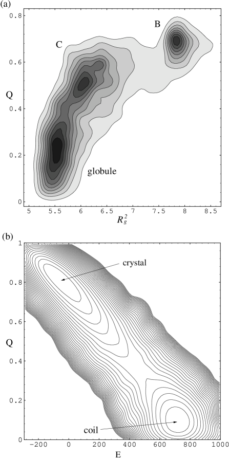
FIG. 7.: (a) Solid-globule coexistence observed for a 100-unit polymer with $\epsilon_{g}=\epsilon$ at $T=0.675\epsilon k^{-1}$. Two-dimensional probability distribution in $Q$ and $R_{g}^{2}$. The labels $B$ and $C$ refer to the global minima of Table I on which the structure of the polymers contributing to the maxima are based. (b) Crystal-coil coexistence for a 343-unit polymer with $\epsilon_{g}=\epsilon$ at $T=3.45\epsilon k^{-1}$. Two-dimensional free energy profile in $Q$ and $E$. The contours occur at intervals of $0.5kT$ above the global free energy minimum. The contours over $15kT$ above the global minimum are not plotted.

This behaviour is similar to simple liquids where decreasing the range of the potential leads to an increasing energy gap between solid and liquid because of the increasing energetic penalty for the disorder associated with the dispersion of nearest-neighbour distances in the liquid, thus playing an important role in the destabilization of the liquid phase.[34, 35]

FIG. 8.: Phase diagram of the 343-unit polymer. The phase diagram is divided into regions by the values of $T_{m}$ and $T_{\theta}$. The position of the heat capacity peak associated with collapse, $T_{c}$, has also been included. The solid lines with data points are simulation results, and the dotted line is from the simple theoretical calculation of $T_{m}$ outlined in Section III B.

The respective roles of energy and entropy in the increase of $T_{m}$ with stiffness can be investigated more quantitatively by approximating the free energy of the disordered state by that for the ideal coil. This is a reasonable approximation, since the ideal expression for $n_{g}$, $n_{g}^{ideal}=4N/(\exp(\beta\epsilon_{g})+4)$, fits the simulation values for the coil, and for the globule, fairly closely. The free energy of an ideal coil $A_{ideal}$ is

$$A_{ideal}=-NkT\log\left(1+4\exp(-\beta\epsilon_{g})\right).$$ (7)

Decomposing this expression into its energetic and entropic components showed that the increase in the energy with stiffness is the main contributor to the change in the free energy of the disordered state with stiffness, except at the higher temperatures relevant to the ‘melting’ transition for larger values of $\epsilon_{g}$.

Use of Equation (7) also allows us to calculate a value of $T_{m}$ if we approximate the free energy of the solid by only its energetic component [Equation (5)]. This simple calculation gives surprisingly good agreement with the simulation data [Figure 8], especially at larger $\epsilon_{g}$. It breaks down at low $\epsilon_{g}$, e.g. the prediction of a non-zero value of $T_{m}$ at $\epsilon_{g}$=0, because Equation (7) is the free energy of a coil in the absence of any interactions; for the dense polymers at low $\epsilon_{g}$ and near to $T_{m}$, the polymer-polymer contacts make a significant contribution to the energy of the disordered state. The number of polymer-polymer contacts in the disordered polymer decreases significantly with increasing temperature, because of the larger entropy of less dense configurations. Therefore, Equation (7) becomes a better approximation to the free energy at higher temperatures, and thus provides a better description of melting at the higher temperatures relevant for larger $\epsilon_{g}$.

Our simulation results for $T_{m}$ are also in qualitative agreement with theoretical results in which a more sophisticated treatment of the globule[15] gives the correct behaviour for $T_{m}$ at low $\epsilon_{g}$. However, a drawback of the description of Doniach et al. is that the free energy of the coil per polymer unit is nonzero in the limit of large $\epsilon_{g}/kT$, causing $T_{m}$ to reach an asymptotic value, rather than continuing to increase with $\epsilon_{g}$.

The increase in $\Delta E$ with stiffness also has an effect on the coexistence of ordered and disordered states. At large values of $\epsilon_{g}$ there is multimodality in the probability distribution for the energy as well as for the order parameter, because of larger free energy barriers between the states. In the example shown in Figure 7b there is a free energy barrier of $3.24kT$ for passing from the crystal to the coil.

A consideration of the effect of size on the transition shows that as the polymer becomes longer the melting point becomes higher, and the transition becomes sharper with an increasing latent heat per monomer [Figure 9b]. This is consistent with the transition being the finite-size analogue of a first-order phase transition. $T_{m}$ increases with size because the effect of the surface term (the $N^{2/3}$ term) in the energy of a crystallite [Equation (5)] diminishes with size. Moreover, as the coefficient of the surface term increases with $\epsilon_{g}$ (the higher aspect ratio crystallites have a larger surface area) the effects of size on $T_{m}$ are more pronounced at larger $\epsilon_{g}$.

FIG. 9.: $C_{v}/N$ as a function of size for (a) $\epsilon_{g}=0$ and (b) $\epsilon_{g}=3\epsilon$.

At $\epsilon_{g}$=0 the behaviour is qualitatively different because there is no energy difference between the orientationally ordered and disordered forms. As there are far fewer states that possess orientational order, they are never thermodynamically favoured and so there is no orientational order-disorder transition and $Q$ always has a low value [Figure 6a]. Despite this, the polymers we studied do have a low temperature heat capacity peak at $T\sim 0.4\epsilon k^{-1}$ [Figure 9a]. This feature stems from a transition between the maximally compact cuboidal global minimum and a more spherical dense globule, and gives rise to bimodality in the canonical probability distribution of the energy. However, the latent heat per atom for the transition decreases with increasing size, indicating that the transition is not tending to a first-order phase transition in the bulk limit. Furthermore, the form of the heat capacity can be very different for sizes at which it is not possible to form complete cuboids.

The order-disorder transition observed by Zhou et al. was also for a fully flexible polymer.[10] However, as the model used was off-lattice, unlike in our model, there is the possibility of a first-order transition associated with the condensation of the monomers onto a lattice.

C The globule to coil transition

For polymers, there can be two disordered phases, the dense globule [Figure 3c] and the coil [Figure 3d]. They are differentiated by the scaling behaviour of the size of the polymer in each phase. For the globule $R_{g}^{2}\propto N^{2/3}$ and for the coil $R_{g}^{2}\propto N^{6/5}$. Between these two states is the $\theta$-point where $R_{g}^{2}\propto N$ and the polymer is said to behave ideally. On passing from the coil to the globule the polymer collapses, as seen in the sigmoidal shapes of the $R_{g}^{2}$ curves [Figure 10a]. The collapse transition can also give rise to a high temperature peak in the heat capacity, which is more rounded than that for melting and the latent heat of which is associated with the loss in polymer-polymer contacts on going to the lower density coil [Figure 9a]. These features are most clear at $\epsilon_{g}=0$ where they are not obscured by the features due to the melting transition. At higher values of $\epsilon_{g}$ the sigmoidal shape of $R_{g}^{2}$ is cut off at low temperatures by the rise associated with the transition to the crystalline states [Figure 4], and the collapse transition just causes a high temperature shoulder in the heat capacity [Figure 6b]. As the size of the polymer increases the transition becomes sharper with a steeper rise in $R_{g}^{2}$ [Figure 10a] and a narrower heat capacity peak at a higher temperature [Figure 9a]. In the limit $N\rightarrow\infty$ this heat capacity peak occurs at the $\theta$-point.

FIG. 10.: $R_{g}^{2}/N$ as a function of size for (a) $\epsilon_{g}=0$ and (b) $\epsilon_{g}=3\epsilon$.

To complete the phase diagram for our model polymer we estimated $T_{\theta}$ by making use of the scaling relations: a series of plots of $R_{g}^{2}/N$ should all cross at $T_{\theta}$. However, due to finite size effects the value obtained by this method only approaches the exact $T_{\theta}$ (from below) as $N\rightarrow\infty$. For example, we estimate $T_{\theta}(\epsilon_{g}$=0)=3.537 from the crossing point of the lines for $N$=216 and 343, whereas an accurate determination gives $T_{\theta}$=3.721.[3]

Figure 8 shows that $T_{\theta}$ has only a weak dependence on $\epsilon_{g}$. Combined with the increase of $T_{m}$ with $\epsilon_{g}$, this leads to the loss of the globular phase at $\epsilon_{g}\sim 12\epsilon$. Above this value the polymer passes directly between the solid and the coil phases, i.e. there is only one disordered phase. An analogy can be made to the phase behaviour of simple atomic systems, with a correspondence between the dense globule and the liquid and between the coil and the vapour. For both systems the denser phase disappears as an interaction parameter is varied, for polymers as the stiffness is increased and for atomics systems as the range of the potential is decreased.[36]

Our phase diagram is consistent with the work of Bastolla and Grassberger. From simulations of polymers longer than those we study here, they found that the globular phase disappears at $\epsilon_{g}\sim 13\epsilon$.[16] The phase diagrams is also very similar to the theoretical predictions of Doniach et al. who estimate the loss of the globular phase to occur at $\epsilon_{g}\sim 15\epsilon$.[15] However, they assumed that $T_{\theta}$ is constant whereas both in ref. [16] and here a small increase with $\epsilon_{g}$ is observed.

Precursors of the loss of the globular phase can be seen at $\epsilon_{g}<12$. These effects are due to finite size, and for smaller polymers they occur at lower values of $\epsilon_{g}$. Firstly, the features in the heat capacity due to collapse become engulfed by the peak due to melting. As the stiffness increases, the collapse peak becomes only a shoulder and then it disappears altogether [Figure 6b]. Secondly, on melting the polymer can pass directly from the solid to a low density disordered state, albeit one where $R_{g}^{2}$ scales less than linearly with size. This effect can be seen for the 27-unit polymer at $\epsilon_{g}=3\epsilon$ [Figure 10], and is also seen for longer polymers at larger values of $\epsilon_{g}$ [Figure 4a]. It results from the expansion of sufficiently stiff and small polymers with decreasing temperature, which is because the persistence length becomes a significant fraction of the total length. An estimate of the persistence length is given by the ratio $N/n_{g}$, the average length between gauche bonds, $N/n^{ideal}_{g}=1+\exp(\beta\epsilon_{g})/4$.

Considerable theoretical effort has gone into studying the evolution of the coil–globule transition as the stiffness of the polymer is increased, see Refs. [37, 38] and references therein. The theories predict that the coil–globule transition is second order for flexible polymers (this has been confirmed by simulation[3]) but becomes first order as the stiffness increases. Due to the small size of the polymers we have simulated we are unable to determine the order of the transition accurately and so cannot test this prediction. However, the theories all assume a liquid-like dense phase; they neglect the possibility of an ordered dense phase, despite it being well known that the dense state of DNA, a stiff polymer, has hexagonal order.[39, 40] It is clear from Figure 8 that for stiff polymers, the coil–globule transition is preempted by a coil–solid transition.

The difference in phase behaviour between flexible and stiff polymers can be easily understood. As a flexible polymer is cooled, the Boltzmann weight for polymer-polymer contacts increases and so the number of contacts increases, at a cost in the entropy of the polymer. The entropy cost derives from the fact that the polymer must bend back on itself in order for the units to be in contact. The increase in the number of contacts is continuous and so the radius of gyration of the polymer varies continuously — the coil–globule transition is second order. However, bending a stiff polymer back on itself is more difficult, it costs both entropy and energy. This larger cost can be repaid if more than one pair of units is in contact, which is true if the two parts of the polymer run parallel to each other for several units. Of course, as the polymer is stiff the entropy cost for two parts of the polymer to run parallel for a number of units is small. The low energy configurations of a stiff polymer are those with long parts of the polymer parallel, see Section IIA. The energy gain is even larger if a number of parts of the polymer form a bundle,[41, 42] e.g. if four parts of the polymer which are running parallel form a square bundle the energy is not twice but four times that of two parts running parallel. So, when the polymer is cooled below the point where the energy gain of bundles outweighs their entropy cost then these bundles proliferate and the radius of gyration drops suddenly — the coil–solid transition is first order.

Our results can also be related to experiment. The coil-globule transition of polystyrene, a flexible polymer, is continuous and the globule is liquid-like.[37, 43] For DNA, an example of a stiff polymer, a first-order transition has been observed between the coil and a compact dense state,[39, 44] which has hexagonal order.[39, 40] The lattice model used here also has a continuous [3] coil–globule transition when $\epsilon_{g}/\epsilon$ is small and a first-order transition from a coil to an ordered dense state when $\epsilon_{g}/\epsilon$ is large. It is thus able to reproduce the phenomenology of the existing experimental data. However, we do not know of any examples where the three phases—coil, globule and crystalline—predicted by our model to occur for semi-flexible polymers have been experimentally observed.

IV Conclusion

In this paper we have provided an example of an order-disorder transition that can be observed for an isolated homopolymer. Its basis in the interactions of the model is clear. The global minimum is orientationally ordered in order to minimize the energetic penalty for gauche bonds. At some finite temperature this order must be lost in a transition to the higher entropy globule or coil. As the stiffness of the polymer increases the energy gap between the ordered and disordered states increases contributing to an increase in the temperature at which this ‘melting’ transition occurs. This effect, coupled with the weak dependence of the $\theta$-point on the stiffness parameter, leads to the disappearance of the disordered globule for sufficiently stiff polymers; there is no longer a collapse transition from the coil to globule. This behaviour is analogous to the disappearance of the liquid phase of simple atomic systems as the range of the potential is decreased. The phase diagram we obtain is in good agreement with recent theoretical[15] and simulation[16] studies of this polymer model.

One of the intriguing aspects of our model is the folded structures that form at low temperature. Firstly, these states are not artifacts of our lattice model. In simulations of isolated polyethylene chains, for the same energetic reasons as in our model—the extra energy from polymer-polymer contacts outweighs the energetic cost of forming a fold—relaxation to folded structures was observed.[22, 23] Furthermore, as here, it was also found that the aspect ratio of the crystallites increased with increasing stiffness.[23] However, we know of no experiments on a homopolymer system where evidence has been found for a transition from a disordered globule to a crystalline structure with chain folds. The most likely signature for such a transition would be an increase in the radius of gyration with decreasing temperature in very dilute polymer solutions.

It is also natural to ask whether this study can provide any insights into polymer crystallization, since polymer crystals have a lamellar morphology in which the polymer is folded back and forth in a similar manner to the folded structures we observe. However, the formation of the folded structures for the isolated polymer is a purely thermodynamic effect—the structures are the global minima—whereas in the bulk case it is a kinetic effect[45, 46]—it is generally accepted that the global minimum is a crystal where all the chains are in an extended conformation. The study, though, may have a more indirect relevance to the crystallization of polymers from solution. Although little consideration has been given to the structure of the polymer arriving at the surface in theories of polymer crystallization, it is not implausible that the existence of significant ordering in the adsorbing polymer would have a considerable effect on the crystallization process.

Although the present study only examines the homopolymer thermodynamics, some comments concerning the dynamics can be made. Klimov and Thirumalai made the interesting observation that model proteins are most likely to be good folders when $T_{f}/T_{\theta}$ is large, where $T_{f}$ is the temperature at which the transition to the native state of the protein occurs.[47] For our system $T_{m}/T_{\theta}$ increases with $\epsilon_{g}$ [Figure 8]. Therefore, if Klimov and Thirumalai’s relation also holds for our homopolymers, one would expect crystallization of the polymer to become more rapid as the stiffness increases—crystallization is easier direct from the coil than via the disordered dense globule. However, whereas at $T_{f}$ there is a transition to a single state, the globule minimum, at our $T_{m}$ a transition to an ensemble of crystalline structures occurs. Therefore, it does not necessarily follow that the homopolymers would be able to reach the global minimum more rapidly as the stiffness increased—indeed it might be that trapping in low-lying crystalline structures is more pronounced for stiff polymers.

- [1] P. J. Flory, Principles of Polymer Chemistry (Cornell University, Ithaca, 1967).
- [2] P. G. de Gennes, Scaling Concepts in Polymer Physics (Cornell University, Ithaca, 1979).
- [3] P. Grassberger and R. Hegger, J. Chem. Phys. 102, 6681 (1995).
- [4] R. S. Berry, T. L. Beck, H. L. Davis, and J. Jellinek, Adv. Chem. Phys. 70, 75 (1988).
- [5] P. Labastie and R. L. Whetten, Phys. Rev. Lett. 65, 1567 (1990).
- [6] O. H. Nielsen et al., Europhys. Lett. 26, 51 (1994).
- [7] J. P. K. Doye and D. J. Wales, Phys. Rev. Lett. submitted (1997).
- [8] R. M. Bradley, Phys. Rev. E 48, R4195 (1993).
- [9] Y. A. Kuznetsov, E. G. Timoshenko, and K. A. Dawson, J. Chem. Phys. 104, 336 (1996).
- [10] Y. Zhou, C. K. Hall, and M. Karplus, Phys. Rev. Lett. 77, 2822 (1996).
- [11] A. Kolinski, J. Skolnick, and R. Yaris, J. Chem. Phys. 85, 3585 (1986).
- [12] A. Kolinski, J. Skolnick, and R. Yaris, Proc. Natl. Acad. Sci. USA 83, 7267 (1986).
- [13] A. Kolinski, J. Skolnick, and R. Yaris, Biopolymers 26, 937 (1987).
- [14] I. Szleifer, E. M. O’Toole, and A. Z. Panagiotopoulos, J. Chem. Phys. 97, 6802 (1992).
- [15] S. Doniach, T. Garel, and H. Orland, J. Chem. Phys. 105, 1601 (1996).
- [16] U. Bastolla and P. Grassberger, preprint (1997).
- [17] W. J. C. Orr, Trans. Faraday Soc. 43, 12 (1947).
- [18] W. Bruns, Macromolecules 17, 2826 (1984).
- [19] H. Meirovitch and H. A. Lim, J. Chem. Phys. 92, 5144 (1990).
- [20] M. C. Tesi, E. J. Janse van Rensburg, E. Orlandini, and S. G. Whittington, J. Phys. A 29, 2451 (1996).
- [21] A. Keller, Rep. Prog. Phys. 31, 623 (1968).
- [22] T. A. Kavassalis and P. R. Sundararajan, Macromolecules 26, 4144 (1993).
- [23] P. R. Sundararajan and T. A. Kavassalis, J. Chem. Soc., Faraday Trans. 91, 2541 (1995).
- [24] S. Fujiwara and T. Sato, J. Chem. Phys. 107, 613 (1997).
- [25] J. I. Siepmann and D. Frenkel, Mol. Phys. 75, 59 (1992).
- [26] M. Dijkstra, D. Frenkel, and J. P. Hansen, J. Chem. Phys. 101, 3179 (1994).
- [27] R. Ramakrishnan, B. Ramachandran, and J. F. Pekny, J. Chem. Phys. 106, 2418 (1997).
- [28] J. M. Deutsch, J. Chem. Phys. 106, 8849 (1997).
- [29] T. Ishinabe, J. F. Douglas, A. M. Nemirovsky, and K. F. Freed, J. Phys. A 27, 1099 (1994).
- [30] J. F. Douglas, C. M. Guttman, A. Mah, and T. Ishinabe, Phys. Rev. A 55, 738 (1997).
- [31] A. M. Ferrenberg and R. H. Swendsen, Phys. Rev. Lett. 63, 1195 (1989).
- [32] R. Poteau, F. Spiegelman, and P. Labastie, Z. Phys. D 30, 57 (1994).
- [33] R. R. Hudgins, P. Dugourd, J. M. Tenenbaum, and M. F. Jarrold, Phys. Rev. Lett. 78, 4213 (1997).
- [34] J. P. K. Doye and D. J. Wales, Science 271, 484 (1996).
- [35] J. P. K. Doye and D. J. Wales, J. Phys. B 29, 4859 (1996).
- [36] M. H. J. Hagen and D. Frenkel, J. Chem. Phys. 101, 4093 (1994).
- [37] A. Y. Grosberg and D. V. Kuznetsov, Macromolecules 25, 1970 (1992).
- [38] C. Williams, F. Brochard, and H. L. Frisch, Ann. Rev. Phys. Chem. 32, 433 (1981).
- [39] L. S. Lerman, Proc. Natl. Acad. Sci. USA 68, 1886 (1971).
- [40] J. Ubbink and T. Odijk, Biophys. J. 68, 54 (1995).
- [41] R. P. Sear, Phys. Rev. E 55, 5820 (1997).
- [42] R. P. Sear, J. Chem. Phys. in press (1997).
- [43] S.-T. Sun, I. Nishio, G. Swislow, and T. Tanaka, J. Chem. Phys. 73, 5971 (1980).
- [44] M. Ueda and K. Yoshikawa, Phys. Rev. Lett. 77, 2133 (1996).
- [45] J. D. Hoffman, G. T. Davis, and J. I. Lauritzen, in Treatise on Solid State Chemistry, edited by N. B. Hannay (Plenum Press, New York, 1976), Vol. 3, Chap. 7, p. 497.
- [46] K. Armistead and G. Goldbeck-Wood, Adv. Polym. Sci. 19, 219 (1992).
- [47] D. K. Klimov and D. Thirumalai, Phys. Rev. Lett. 76, 4070 (1996).