Fine structure and complex exponents in
power law distributions from random maps

Abstract

Discrete scale invariance (DSI) has recently been documented in time-to-failure rupture, earthquake processes and financial crashes, in the fractal geometry of growth processes and in random systems. The main signature of DSI is the presence of log-periodic oscillations correcting the usual power laws, corresponding to complex exponents. Log-periodic structures are important because they reveal the presence of preferred scaling ratios of the underlying physical processes. Here, we present new evidence of log-periodicity overlaying the leading power law behavior of probability density distributions of affine random maps with parametric noise. The log-periodicity is due to intermittent amplifying multiplicative events. We quantify precisely the progressive smoothing of the log-periodic structures as the randomness increases and find a large robustness. Our results provide useful markers for the search of log-periodicity in numerical and experimental data.

PACS numbers: 02.50.-r, 05.40.+j, 47.53.+n

I INTRODUCTION

Complex critical exponents and complex fractal dimensions have until recently been discussed only for hierarchical systems, be they man-made [1, 2, 3, 4, 5, 6, 7, 8] or naturally occurring as in the mammalian bronchial tree [9, 10]. These hierarchical systems are characterized by discrete scale invariance (DSI), a notion qualitatively similar to the concept of “lacunarity”. A signature of this DSI is the presence of log-periodic oscillations correcting the usual power laws, corresponding to complex exponents.

Recently, their occurrence in irreversible rupture [11, 12, 13, 14, 15, 16] and growth processes [17, 18] as well as prior to financial crashes [19, 20] have been documented. It has been suggested [21] that complex exponents are rather common and should be looked for generically in any model whose critical properties are described by an underlying non-unitary field theory. This excludes the usual homogeneous spin systems in which the renormalization flow is a gradient [22]. This includes models with non-local properties such as percolation and animals [21], polymers and their generalizations, models of irreversible growth processes such as rupture [11, 12, 13, 14, 15, 16], Diffusion-Limited-Aggregation (DLA) [17, 18], and models with quenched disorder like spin-glasses [23, 24, 25, 26, 27]. See [28] for a review.

Three outstanding problems remain :

• do we know all the physical mechanisms that can produce complex critical exponents?

• how strong are the log-periodic structures and how robust are they with respect to noise and disorder?

• does there exist a smooth invariant probability distribution (having a density), or is it discrete?

With respect to the first question, six situations have been discussed :

1. the presence of a built-in geometrical hierarchy [1, 2, 3, 4, 5, 6, 7, 8, 10] ;

2. the diffusion in anisotropic quenched random lattices in which the hierarchy is constructed dynamically due to the probabilistic encounters with traps [29] ;

3. intermittent amplification processes [30] ;

4. cascades of ultra-violet instabilities as in rupture and growth processes [17, 18] ;

5. non-local geometry [21] ;

6. quenched disordered systems [23, 24, 25, 26, 27].

In regards to the second question, log-periodic oscillations of spin systems on a fractal amounts to exceedingly small effects, typically of the order of $10^{-5}$ in relative value [2, 6]. In contrast, it is still not fully understood why log-periodic structures seem to be many times stronger, of the order of $10\%$ or so, in rupture and growth processes. In addition, log-periodicity implies a prefered scaling ratio which, in nature, should be largely perturbed by disorder. Theoretical estimates of the effect of disorder on the log-periodic corrections indicate that they should be generally robust [21]. An important practical question is how much disorder or noise will make the log-periodic corrections too small to be observed. Ensemble averaging is also an issue as finite-size effects cause significant variations in the phase of the log-periodic oscillations. Averaging may cause them to disappear. This was observed in DLA clusters [17] in which single cluster analysis uncovered the log-periodic structures while averaging procedures destroyed them.

In order to address these questions on the effect of disorder, we study a simple, positive, random map with parametric noise ,

$$X_{t+1}=a_{t}X_{t}+b_{t},\;\;\mbox{with}\;a_{t},b_{t}>0\;.$$ (1)

The growth rate $a_{t}$ and the additional term $b_{t}$ are assumed to be pairs of positive identically distributed random values with the joint distribution function ${\cal P}_{a,b}$. In most of the cases treated below, we assume that $a_{t}$ and $b_{t}$ are independent, which yields ${\cal P}_{a,b}={\cal P}_{a}{\cal P}_{b}$.

FIG. 1.: $X_{t}$ history for $a_{t}$ with a two point distribution (section IV) at $a=2$, $\xi=2$, $p=0.95$, and $b_{t}=1$.

It may seem that the linear model (1) is so simple that it does not require a careful mathematical investigation. This is however not the case, as the rather extensive mathematical analysis of the problem in [33] indicates. We will show a very unusual behavior of solutions of the difference equation (1). It is known [33] that, provided some regularity assumptions hold and when the average rate of growth $\langle\ln a_{t}\rangle$ is negative, then the time series $X_{t}$ is stationary. Furthermore $X_{t}$ is characterized statistically by a probability distribution function with a power law tail :

$${\cal P}_{X}(x)\sim x^{-(1+\mu)}\;,$$ (2)

when the equation for $\mu$,

$$\langle a^{\mu}\rangle=1$$ (3)

has a positive solution [31, 32, 33, 34, 35, 36].

The power law distribution function stems from an intermittent and transient amplification occurring when several successive $a_{t}$ are larger than $1$. Its origin is thus in the class of intermittent amplifications [30] and intermittent trapping [29] mechanisms. We may therefore expect complex valued $\mu$ exponents. This should lead to the occurrence of detectable log-periodic corrections in the leading simple power law behavior.

We are here concerned with the continuity or discreteness of this distribution function and with the strength and detection of the potential log-periodic corrections, especially as a function of the distributions ${\cal P}_{a}$ and ${\cal P}_{b}$. Intuitively, the broader these distributions are, the weaker we expect the log-periodic corrections to be since a log-periodicity is the signature of a favored scaling ratio. This preference must disappear as the disorder increases. We aim to carefully quantify this scenario, for the benefit of future analysis of log-periodicity.

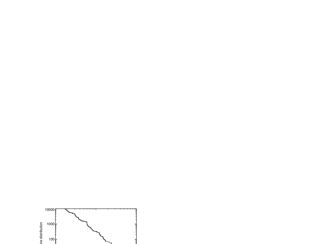
FIG. 2.: Cumulative distribution of the $10^{4}$ largest iterates among $10^{8}$ realized for $a_{t}$ with a two point distribution (section IV) at $a=2$, $p=0.95$, and $b_{t}=1$.

In the next two sections, we recall useful information, discuss a connection with products of random matrices and iterated function systems and review the so-called transition operator approach determining the probability density function (pdf) $P(X)$. We then discuss the case in which $a_{t}$ take only two values ${1/a}$ and $a^{\xi}$ with probability $p$ and $1-p$ respectively, where $a>1$ and $\xi>0$, first in the case of a fixed $b=1$ and then with increasingly widening ${\cal P}_{b}$ distributions. We then analyze the case in which $a_{t}$ is broadly distributed and discuss the detection criteria for the log-periodic corrections.

In addition to the present focus as a paradigm of system exhibiting complex exponents, this random map (1) has been introduced in various contexts, for instance in the physical modelling of 1D disordered systems [31] and the statistical representation of financial time series [32]. The variable $X_{t}$ is known in probability theory as a Kesten variable [33]. The map (1) describes for instance the time evolution of a fish population $X_{t}$ with $a_{t}$ depending on the rate of reproduction and on the depletion rate due to fishing as well as environmental conditions and $b_{t}$ describing the input due to restocking from an external source such as a fish hatchery, or from migration from adjoining reservoirs [36]. The random map (1) can also be applied to other problems of population dynamics, epidemics, investment portfolio growth, and immigration across national borders [36]. Variations of this model have recently been proposed for the analysis of crop control in the presence of weed infestion [37]. Models of enonomic evolution typically involve a system of affine coupled equations of the type (10) below, which are multi-dimensional generalization of (1). For instance, the economic model of Keynes in its simplest form links consumption, investment and production in a linear affine system of deterministic equations. The system (10) corresponds to a generalization in which the coefficients of the auto-regression are allowed to fluctuate in time to account for uncertainty. More generally, models used in econometrics [38] are very similar to (1) and (10) below, even if they usually assume constant coefficients.

It is probably true that (1) is one of the simplest linear stochastic equation that can provide an alternative modeling strategy for describing complex time series. We note that a nonlinear version with a quadratic nonlinearity (corresponding to the logistic equation with random multiplicative noise) has recently been shown to lead to a new type of crisis, in that there is a sudden qualitative change in the chaotic dynamical behavior induced by variations of the parameters [39]. We do not discuss these properties but restrict our considerations to the affine random map (1).

II RESULTS ON THE KESTEN AFFINE RANDOM MAP

A Formal solution

The formal solution of (1) for $N\geq 1$ reads

$$X_{t+N}=(\prod_{l=0}^{N-1}a_{t+l})X_{t}+\sum_{l=0}^{N-1}b_{t+l}\prod_{m=l+1}^{N-1}a_{t+m}\;,$$ (4)

where we define $\prod_{m=N}^{N-1}a_{t+m}\equiv 1$ for the special value $l=N-1$. It is clear that the $\prod_{l=0}^{N-1}a_{t+l}$ multipliers of (4) control the $X_{t}$ dynamics. Thus, $X_{t+N}$ diverges (resp. remains bounded) if the average logarithmic growth factor $\langle\ln a_{t}\rangle$ is positive (resp. negative). Here, we focus our attention on the case

$$\langle\ln a_{t}\rangle<0\;.$$ (5)

In this regime, we notice the role of $b_{t}$ which provides a reinjection mechanism [34] allowing $X_{t}$ to fluctuate without converging to zero, as it would if $b_{t}$ vanished.

B Product of random matrices

The map (1) can be written as a product of random $2\times 2$ matrices :

$$\left(\begin{array}[]{c}X_{t+1}\\ 1\end{array}\right)=\left(\begin{array}[]{cc}a_{t}&b_{t}\\ 0&1\end{array}\right)\left(\begin{array}[]{c}X_{t}\\ 1\end{array}\right)\;.$$ (6)

By Furstenberg’s theorem, the norm $||V_{t}||$ ($\sim X_{t}$ for large $X_{t}$) of the $t$-th vector

$$V_{t}\equiv\left(\begin{array}[]{c}X_{t}\\ 1\end{array}\right)$$ (7)

grows as [40]

$$||V_{t}||=||V_{0}||e^{\lambda_{1}t}\;,$$ (8)

where $\lambda_{1}$ is the largest Lyapunov exponent of the product of the random matrices. The $2\times 2$ matrices are triangular and thus

$$\lambda_{1}=\max\{\langle\ln a_{t}\rangle,\,0\}\;.$$ (9)

We recover the exponential growth regime of $X_{t}$ for $\langle\ln a_{t}\rangle>0$. In the reverse case, $\langle\ln a_{t}\rangle<0$, the Lyapunov exponent is zero, which corresponds to the marginal case between exponential growth and exponential decay. This is the regime where one usually encounters power law behavior, for instance in power law sensitivity to initial conditions in dynamical systems at the onset of chaos [42].

It is worth noticing that this zero Lyapunov exponent is different from the directly measured Lyapunov exponent of (1). Indeed, the solution (4) shows that a perturbation $\delta X_{t}$ at time $t$ gives an error $\delta X_{t+N}=\delta X_{t}\prod_{l=1}^{N-1}a_{t+l}\sim e^{(N-1)\langle\ln a\rangle}$. This corresponds to a negative Lyapunov exponent for the case studied here (5), equal to $\langle\ln a\rangle$. This would lead one to conclude that the dynamics is trivial. Generally speaking, the widespread opinion in the physical community that notions like chaos, etc., have some strict correspondence to the positivity of Lyapunov exponents is not quite correct. See, for example, the detailed discusssion of nonchaotic dynamical systems with positive Lyapunov exponents and vice versa, and futher references in [43, 44]. Here, the usual calculation of the Lyapunov exponent is not sensitive to the “reinjection” mechanism brought by the $b_{t}$ term. By construction, the matrix formulation (6) takes this effect into account. The resulting vanishing Lyapunov exponent alerts us to the possibility of complex behavior.

C Iterated Function System

We also mention the relationship with Iterated Function Systems (IFS), which are defined as follows [45]. One first defines an affine transformation $W$ from $R^{D}$ to $R^{D}$:

$$W[{\bf x}]={\bf Ax}+{\bf b}\;,$$ (10)

where ${\bf A}$ is a $D\times D$ matrix and ${\bf b}$ a vector in $R^{D}$. An affine transformation is contractive if there exists a Lipschitz constant $s<1$ such that

$$|W[{\bf x}]-W[{\bf y}]|<s|{\bf x}-{\bf y}|\;.$$ (11)

An IFS consists of $N$ affine transformations $W_{i}$ and a set of probabilities $p_{i}>0$ with $\sum_{i=1}^{N}p_{i}=1$. Starting with a given set of points, the IFS code consists in applying to it an infinite sequence of transformations, each of them being chosen with its corresponding probability. In general, IFS codes satisfy the average contractive condition :

$$s_{1}^{p_{1}}s_{2}^{p_{2}}\cdots s_{N}^{p_{N}}<1\;.$$ (12)

Taking $D=1$, we see that (10) is the same as (1), where $N$ is the number of different values taken by $a_{t}$ (suppose for simplicity that $b_{t}$ is constant) with their respective probabilities $p_{i}$. In other words, the affine random map (1) is a one-dimensional IFS. Then, the Lipschitz constant $s_{i}$ is equal to the $i$-th value $a_{i}$ that $a_{t}$ can take. Condition (12) then becomes the familiar

$$\sum_{i=1}^{N}p_{i}\ln a_{i}\equiv\langle\ln a\rangle<0\;.$$ (13)

This retrieves the regime (5) discussed above. Usually, IFS are studied in situations where all the affine transformations have their Lipschitz constant individually negative, i.e. all are contractive. The present work (where $D=1$) deals with a rather special but very interesting situation where some of them are dilating, while on average the set of transformations is contractive. This correspondence and the discovery that power law distributions are found when some of the transformations of the IFS are dilating suggests to us an investigation of the behavior of similar intermittent dilating IFS in higher dimensions, where rotations are added to the translation and dilation processes. This is left for future work. Here we will next use the correspondence with IFS to understand intuitively the fractal structures found when the $a_{t}$ take a finite number of values.

D Probability density function

Calling $P_{a_{t}}$, $P_{b_{t}}$, and $P_{X_{t+1}}$ the pdf’s of $a_{t}$, $b_{t}$, and $X_{t+1}$ respectively (and assuming that they are integrable functions), then the pdf of $X_{t}$ (obtained by the standard Markov argument) obeys the following equation :

$$P_{X_{t+1}}(X) = \int_{-\infty}^{\infty}P_{a_{t}}(a)d{a}\int_{-\infty}^{\infty}P_{b_{t}}(b)d{b}$$ (15)

$$\mbox{}\times\int_{-\infty}^{\infty}P_{X_{t}}(Y)\delta(X-aY-b)d{Y}\;,$$

or

$$P_{X_{t+1}}(X)=\int_{-\infty}^{\infty}{P_{a_{t}}(a)\over a}d{a}\int_{-\infty}^{\infty}P_{b_{t}}(b)P_{X_{t}}({{X-b}\over{a}})d{b}\;.$$ (16)

The two pdfs $P_{X_{t}}$ and $P_{X_{t+1}}$ approach a common stationary pdf, $P(X)$, for large $t$ [34, 35]. We are interested in the description of the tail of $P(X)$, i.e. for $X\gg b$. We can then neglect the $b$ term of $P_{X_{t}}((X-b)/{a})$ in the r.h.s. of (16). This allows us to simplify (16) into

$$P(X)=\int_{-\infty}^{\infty}{P_{a_{t}}(a)\over a}P({X\over a})d{a}\quad\mbox{for large}\quad X\;,$$ (17)

using $\int_{-\infty}^{\infty}P_{b_{t}}(b_{t})d{b_{t}}=1$. Since (17) is linear in $P(X)$, the general solution can be written as a sum over a set of particular solutions [31]. These solutions are composed of power laws and faster decaying functions (exponentials). The set of power law solutions is obtained by assuming the form $P(X)\sim X^{-(1+\mu)}$ for $X\gg 1$. This yields (3) determining the exponent $\mu$.

The inequality (5) and the equation (3) are the corner stones of our analysis. We construct and analyze several examples whose parameters are constrained by (5) and we study the solutions of (3) and compare them to direct numerical simulations.

III TRANSITION OPERATOR APPROACH

One of the obstacles in the implementation of the approach in the previous section is that we need to assume that all the considered distributions have densities, which is not the case with at least some of our examples. To study a more general situation, let us consider the so-called transition operator approach.

A Transition operator approach and non-smooth distributions

According to our definitions, (1) defines a Markov chain. We can define the transition operator ${\bf P}$ of this random process as :

$${\bf P}h(x)=\int h(\frac{x-b}{a})\,d{\cal P}_{a,b}(a,b)$$ (18)

for any integrable function $h$. This operator describes the image of a distribution density under the action of our random process. If an invariant probability density $P$ exists it should satisfy

$${\bf P}P=P\;.$$ (19)

The introduction of (18) is justified by the fact that this integral operator allows for the study of non-smooth and even discontinous distributions.

Consider a simple implementation of a random selection scheme. Assume that $0<a_{1}<1<a_{2}$, $0<b_{1}$, $0<b_{2}$ for the two maps :

$$x \to a_{1}x+b_{1}\,$$ (20)

$$x \to a_{2}x+b_{2}\,$$ (21)

such that (20) is chosen with the probability $p$, while (21) is chosen with the probability $1-p$. The corresponding joint distribution ${\cal P}_{a,b}$ for the random variables $a_{t}$ and $b_{t}$ is singular. Furthermore, these two random variables heavily depend on each other. Therefore (16) cannot directly be used. However it is trivial to specify the corresponding transition operator :

$${\bf P}h(x)=\frac{p}{a_{1}}h(\frac{x-b_{1}}{a_{1}})+\frac{1-p}{a_{2}}h(\frac{x-b_{2}}{a_{2}})\;.$$ (22)

Moreover, this description is easily generalized to the case with an arbitrary (albeit finite) number of linear maps $x\to a_{i}x+b_{i}$, where each is selected with the probability $p_{i}$ (provided $\sum_{i}p_{i}=1$),

$${\bf P}h(x)=\sum_{i}\frac{p_{i}}{a_{i}}h(\frac{x-b_{i}}{a_{i}})\;.$$ (23)

The representation (23) shows that our random system lacks a smooth (and even bounded) invariant density for any choice of the positive coefficients $a_{i}$ and $b_{i}$. Assume on the contrary that such pdf $h(x)$ exists. This has to satisfy ${\bf P}h(x)=h(x)$ for any $x\in[0,1]$. To proceed further, we need to estimate the variation of the image of the $h$ function. The variation of a function is, roughly speaking, an integral of the modulus of the derivative of the function over its domain. In the case of monotonic functions, it can be shown that

$${\rm var}({\bf P}h)={\rm var}(h)\sum_{i}\frac{p_{i}}{a_{i}}\;.$$ (24)

According to (12), we note that

$$\prod_{i}a_{i}^{p_{i}}<1\;,$$ (25)

which yields

$$\sum_{i}\frac{p_{i}}{a_{i}}>1\;.$$ (26)

Therefore, each time we apply the transition operator, the variation of the image of a function is multiplied by the factor $\sum_{i}\frac{p_{i}}{a_{i}}>1$. Hence the limit distribution (if it exists) cannot be a function of bounded variation.

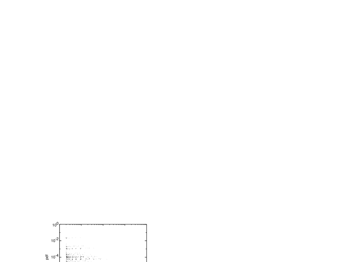
FIG. 3.: The (numerically obtained) pdf for $a_{t}$ with a two point distribution (section IV) at $a=2$, $\xi=2$, $p=0.95$ and $b_{t}=1$ ($10^{8}$ iterates, $10^{4}$ equispaced bins per unit of $\log X_{t}$).

A special case was treated in [31] with a finite system of random maps producing a discrete invariant distribution :

$$x \to 1\qquad\hbox{with probability}\quad p\;,$$ (27)

$$x \to ax+1\qquad\hbox{with probability}\quad 1-p\;.$$ (28)

In this case, it is easy to find the invariant distribution analytically. However, since the first map has a zero value of the multiplier $a$, the system does not satify our assumptions that all coefficients should be positive.

B Existence of pdf for the case of the smooth distribution of coefficients

In this subsection, we study a more general case, where we have a random map $x\to ax+b$ with random coefficients $a,b$, whose joint probability distribution is ${\cal P}(a,b)$. The case considered above corresponds to the discrete distribution ${\cal P}(a,b)$. Our main aim here is to prove that, if the distribution ${\cal P}(a,b)$ has a density $p(a,b)$ with “good enough” properties, then the random map system also has a finite invariant density. Indeed, consider the corresponding transition operator:

$${\bf P}h(x)=\int\int\frac{p(a,b)}{a}h(\frac{x-b}{a})\,da\,db\;.$$ (29)

After the change of variables $\xi=x-b$ this operator becomes

$${\bf P}h(x)=-\int\int\frac{p(a,x-\xi)}{a}h(\frac{\xi}{a})\,da\,d\xi\;.$$ (30)

Assume now that

$${\rm var}_{b}p(a,b)\leq C<\infty$$ (31)

for any $a>0$, where ${\rm var}_{b}p(a,b)$ stands the variation of the $p(a,b)$ function with respect to the second variable. Using the above representation, we find that

$${\rm var}({\bf P}h) \leq \int\int\frac{C}{a}h(\frac{\xi}{a})\,da\,d\xi=C\int\left(\int h(\frac{\xi}{a})\,d(\frac{\xi}{a})\right)\,da$$ (32)

$$= C(\int h(x)\,dx)\int da\;.$$ (33)

Since $h$ is assumed to be the density of a probability distribution, then $\int h(x)\,dx$ is finite. This shows that the variation of ${\bf P}h$ is universally bounded from above. The existence of the invariant distribution [33] then proves the existence of the pdf.

C Markov dependent choice of the subsequent map

Our earlier discussion of random map systems assumed that the choice of a subsequent map $x\to a_{i}x+b_{i}$ does not depend on the immediatly antecedent map chosen. This is a relatively strong restriction and in this section we shall show that this assumption is not necessary. We will show that, for the stationary process, the representation of the transition operator depends only on the stationary probabilities of the random choices $p_{i}$ and not on the transition probabilities between subsequent maps.

Assume that currently the map $x\to a_{i}x+b_{i}$ was chosen, then the conditional probability to choose the map $x\to a_{j}x+b_{j}$ is equal to $p_{ij}$. The process of the random choice is governed by the finite state Markov chain with the transition probabilities $(p_{ij})$. Assume that this Markov chain is ergodic and denote by $p_{i}$ its unique invariant distribution. Then our entire system is still a Markov chain, whose transition operator is:

$${\bf P}h(x)=\sum_{i}p_{i}\left(\sum_{j}\frac{p_{ij}}{a_{j}}h(\frac{x-b_{j}}{a_{j}})\right)$$ (34)

$$= \sum_{j}\frac{1}{a_{j}}h(\frac{x-b_{j}}{a_{j}})\sum_{i}p_{i}p_{ij}=\sum_{j}\frac{p_{j}}{a_{j}}h(\frac{x-b_{j}}{a_{j}})\;.$$ (35)

It depends only on the stationary probabilities $p_{i}$. As a result, we immediately see that all asymptotic properties also depend only on the choice of $p_{i}$.

The generalization of our argument for the general case where the joint distribution of the coefficients $a$ and $b$ may have both discrete and continuous components is straightforward.

IV TWO-POINT DISTRIBUTIONS

Let us return now to the question about the asymptotic (as $x\to\infty$) properties of pdf for the case of only two linear maps. The above derivations show that these asymptotic properties do not depend on the choice of the additional terms $b_{i}$ (as long as they are non-zero and well-behaved). Let

$$a>1,\quad 0<p<1,\quad\mbox{and}\quad\xi>0\;,$$ (36)

such that $a_{1}=1/a<1$ and $a_{2}=a^{\xi}>1$. Equation (17) becomes

$$P(X)=paP(aX)+(1-p)a^{-\xi}P(a^{-\xi}X)\;.$$ (37)

Condition (5) imposes the requirement

$${\xi\over 1+\xi}<p<1\;,$$ (38)

and equation (3) leads to

$$(1-p)z^{1+\xi}-z+p = 0,$$ (39)

$$\qquad\mbox{where}\;z \equiv a^{\mu}\;\mbox{and $z$ complex}\;.$$ (40)

A $\xi$ integer

At first take $\xi=1$, then from (38), we see that $p$ must be within ${1\over 2}<p<1$. The two real solutions of (40) are $z_{\pm}={1\pm\sqrt{\Delta}\over 2(1-p)}$, where $\Delta=1-4p(1-p)\geq 0$. From the definition $z=a^{\mu}$ (and $e^{i2n\pi}=1$ for any integer n), we obtain

$$\mu_{\pm,n}\equiv\mu_{R}+i\mu_{I}={\ln z_{\pm}\over\ln a}+i{2\pi n\over\ln a}\;.$$ (41)

The pdf of $X_{t}$ is thus of the form

$$P(X_{t})=\sum_{\pm,n}{C_{\pm,n}\over X_{t}^{(1+\mu_{R})}}\cos(\mu_{I}\ln X_{t})\;.$$ (42)

The prefered scaling ratios are obtained by the factors of $X_{t}$ reproducing the same values of the cosine, i.e. $a^{1\over n}$, with $n$ integer. The discrete scale invariance is simply the result of the intermittent amplification by the fixed factor $a$. The log-periodicity is thus trivially associated with the discrete multiplicative structure.

When $\xi=2$, three real $z$ solutions exist for $z$, for the allowed range ${2\over 3}<p<1$. The imaginary part of $\mu$ thus stems from the same technical reason as for $\xi=1$ and reflects the intermittent amplification by the factor $a^{2}$.

In general if $\xi=N$ is a positive integer, (40) obeys

$$(1-p)z^{N+1}-z+p=0\quad\Leftrightarrow\quad(z-1)Q_{N}(z;p)=0\;,$$ (43)

where

$$Q_{N}(z;p)\equiv(1-p)\sum_{k=1}^{N}z^{k}-p\;.$$ (44)

The root structure of $Q_{N}(z;p)=0$ for $\Re z>0$ is determined with e.g. Routh’s algorithm [41]. It can be shown that for $N<5$, this polynomial has only one root with $\Re z>0$ and that $\Im z=0$ for this single root. However for $N\geq 5$ there always exist roots such that $\Re z>0$ and $\Im z\neq 0$.

To illustrate the integer $\xi$ regime, Fig. 1 shows a segment of the $X_{t}$ history for the case $a=2$, $\xi=2$, $p=0.95$, and a constant $b_{t}=1$. Most iterates are small while rare intermittent excursions explore very large values. The (numerically obtained) cumulative distribution is shown in the log-log plot of Fig. 2.

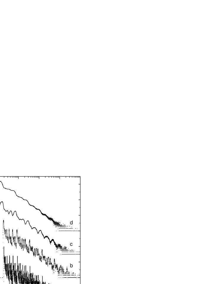
FIG. 4.: The scaled pdf of $X$ given by (1) for $a_{t}$ with two point distribution at $a=2$, $\xi=2$, $p=0.95$, and $b_{t}$ uniform with (a) $1\times{\rm pdf}$ and $\beta={31\over 32}$ ($10^{8}$ iterates, $10^{4}$ equispaced bins per unit of $\log X_{t}$), (b) $10^{3}\times{\rm pdf}$ and $\beta={7\over 8}$ ($10^{9}$ iterates, $10^{3}$ equispaced bins per unit of $\log X_{t}$, the same for (c–d)), (c) $10^{6}\times{\rm pdf}$ and $\beta={1\over 2}$, (d) $10^{9}\times{\rm pdf}$ and $\beta=0$.

A complex structure, reminiscent of a devil staircase, overlays an average linear decay. The structure corresponds to all possible values of $n$ in the imaginary part (41) of the exponent $\mu$, where the largest $n$ provide the smallest details of the cumulative distribution. Figure 3 shows the (numerically obtained) pdf, i.e. the derivative of Fig. 2. We observe a self-similar structure, as expected from the correspondence with the IFS discussed in section II C (IFS in general encode stochastic fractal structures [45]). We also observe that the distribution seems to be nowhere continuous, as expected from the derivation in section III A.

It is interesting to progressively coarse-grain this self-similar structure by introducing a disorder on $b_{t}$. This is accomplished by chosing $b_{t}$ uniformly in the interval $[\beta,1]$. The value $\beta=1$ recovers the ordered case $b_{t}=1$. Decreasing $\beta$ corresponds to increasing the disorder. Figure  4 shows the pdf $P(X_{t})$ for decreasing values $\beta={31\over 32},{7\over 8},{1\over 2},0$ (while keeping $a=2$, $\xi=2$, and $p=0.95$). The roots of (40) are $z_{0}=1$ and $z_{\pm}={-1\pm{\sqrt{7}7}\over 2}$, or $\mu_{R0}=0$, $\mu_{I0}=n{2\pi\over\ln 2}$, $\mu_{R+}\approx 1.9588$, $\mu_{I+}=\mu_{I0}$, $\mu_{R-}\approx 2.5890$, $\mu_{I-}=(1+2n){\pi\over\ln 2}$ for integer $n$.

FIG. 5.: (a) The logarithmic derivative of a portion of the pdf tail for the upper ($\beta=0$) trace in (4). (b) The Lomb periodogram of (a).

The “frequency” of a log-periodic oscillation is defined by

$$f(n)\equiv{\mu_{I}(n)\over{2\pi\log e}}\equiv{1\over\ln\lambda}\;,$$ (45)

where we define $\lambda$ as the scaling ratio associated with the log-periodicity [13, 21]. Here $f(1)_{0}=f(1)_{+}\approx 3.3219$, $f(0)_{-}\approx 1.6609$, and $f(1)_{-}\approx 4.9828$. These numbers are compared to the spectrum analysis of the tail portion of the pdf. We use the logarithmic derivative of the $\beta=0$ pdf of Fig. 4 to get a data with zero average slope (its averave value is the leading power law exponent). This is represented in Fig. 5 a. Its Lomb periodogram spectrum [46] is shown in Fig. 5 b and yields four frequencies $0.6$, $1.6$, $3.3$, and $5.0$. The smallest of these is attributed to the inverse of the (log) tail length used. The others are in good agreement with the predictions $f(0)_{-}$, $f(1)_{+}$, $f(1)_{-}$ in ascending order. The small, partially hidden, bump at $2.1$ and the more recognizable one at $4.3$ are of unknown origin.

B $\xi$ non-integer

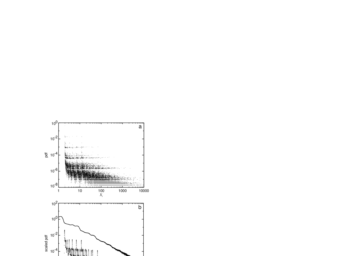
FIG. 6.: (a) The pdf for $a_{t}$ with two point distribution at $a=2$, $\xi=2.5$, $p=0.95$, and $b_{t}=1$ ($10^{8}$ iterates, $10^{4}$ equispaced bins per unit of $\log X_{t}$). (b) The scaled pdfs for $a_{t}$ with two point distribution at $a=2$, $\xi=2.5$, $p=0.95$, $\beta={15\over 16}$ (lower trace, $1\times{\rm pdf}$), and $\beta=0$ (upper trace, $10^{3}\times{\rm pdf}$). Both with $10^{9}$ iterates and $10^{3}$ equispaced bins per unit of $\log X_{t}$.

We have shown that for integer $\xi\geq 5$ there will always exist some roots of (40) with non-zero imaginary and positive real parts. This type of root structure is common for non-integer $\xi$. If $\xi$ is irrational then an infinite number of distinct roots solves (40). We select the slightly simpler case $\xi=2.5$ (with $a=2$ and $p=0.95$ as before).

In Fig. 6 a, the pdf for $b_{t}=1$ is given for the $10^{8}$ first iterates of (1) with a binning density of $10^{4}$ points per decade. Figure 6 b shows the pdf for a uniformly distributed $b_{t}$ with $\beta={15\over 16}$ (lower trace) and the scaled pdf (upper trace, $10^{3}\times{\rm pdf}$) for $\beta=0$, i.e. $b_{t}$ uniformly distributed between $0$ and $1$. These two pdfs use the first $10^{9}$ iterates of (1) with a log-equidistant binning of $10^{3}$ points per decade.

As already pointed out in section III B, a continuous $b_{t}$ distribution seems to lead to a continuous pdf for $X$. The analysis above neglected the influence of a varying $b_{t}$. We resort to a limit consideration on a sequence of progressively thinned, uniform, $b_{t}$ distributions to match theory with the present simulation results. We select the three cases $\beta=0,{3\over 4},{7\over 8}$. For each of these tail regions of the pdf (Fig. 7 a, Fig. 8 a, and Fig. 9 a), the logarithmic derivative is computed (Fig. 7 b, Fig. 8 b, and Fig. 9 b). This gives a local estimate of the leading exponent of the power law tail of the pdf. A constant value would correspond to a pure power law. Oscillations which are approximately periodic in $\ln X$ are the signatures of the log-periodicity. This is confirmed by a spectral analysis given in Fig. 7 c, Fig. 8 c, and Fig. 9 c of the signals shown in Fig. 7 b, Fig. 8 b, and Fig. 9 b respectively, using the Lomb periodogram technique [46]. We clearly identify a number of frequencies. We compare these numerical results with a direct analytical determination of the roots of (3,40). The complex $\mu$ solutions are sought where $z=a^{\mu}=e^{x+iy}$. These are the roots of

$$R(x,y;\xi,p)+iJ(x,y;\xi,p)=0\;,$$ (46)

where

$$R(x,y;\xi,p) \equiv (1-p)e^{(1+\xi)x}\cos((1+\xi)y)$$ (48)

$$\mbox{}-e^{x}\cos y+p\;,$$

$$J(x,y;\xi,p) \equiv (1-p)e^{(1+\xi)x}\sin((1+\xi)y)$$ (50)

$$\mbox{}-e^{x}\sin y\;.$$

The zeroes of (48) and (50) define nodal curves in the $x$–$y$ plane. The solutions $(x,y)$ are the intersections of these nodal curves. When $\xi$ is rational $\xi=M/N$, where $M$ and $N$ are the smallest relative prime positive integers, we see that the set of solutions is periodic in the $y$-direction with a period $2\pi N$. The two equations (48,50) are converted into

$$(1-p)e^{\xi x} = {\sin y\over\sin(1+\xi)y}\;,$$ (51)

$$e^{x} = p{\sin(1+\xi)y\over\sin\xi y}\;.$$ (52)

This shows that the values of $x$ are bounded from above by a finite number. An unbounded $x$ would from (52) correspond to a vanishing $\sin\xi y$. This would imply that $\xi y=n\pi$, for some integer $n$, and therefore that $\sin(1+\xi)y=(-1)^{n}\sin y$. Using (51) we would obtain $(1-p)e^{\xi x}=1$ ($n$ odd is not allowed) leading to a contradiction. This implies that there is a maximum value for $\mu_{R}$. Table I gives the five solutions $(x_{m},y_{m})$, indexed by $m=1$ to $5$. For a given $m$, we also extract the few first solutions obtained by $4\pi$ periodic repetitions in the $y$ direction. These solutions are indexed by an additional integer $n$ corresponding to the order of the $4\pi$ period. We give these solutions in the $\mu_{R}$ and $\mu_{I}$ parameter space.

TABLE I.: All roots $x$, $y$, and the first few $\mu=\mu_{R}+i\mu_{I}$ roots (here $a^{\mu}=e^{x+iy}$) of (48, 50) for $a_{t}$ with two point distribution at $a=2$, $\xi=2.5$, and $p=0.95$.

$m$	1	2	3	4	5
$x(m)$	1.03	1.28	1.19	1.19	1.28
$y(m)$	0.0	2.56	4.91	7.66	10.06
$\mu_{R}(m)$	1.47	1.85	1.72	1.72	1.85
$\mu_{I}(m,n=0)$	0.0	3.69	7.08	11.04	14.43
$\mu_{I}(m,n=1)$	18.13	21.82	25.21	29.18	32.57
$\mu_{I}(m,n=2)$	36.26	39.95	45.34	47.31	50.69
$\mu_{I}(m,n=3)$	54.39	58.08	61.47	65.43	68.82

The appendix provides an approximate but quite accurate analytical determination of the solutions found in this table, based on a perturbative scheme. The pdf of $X_{t}$ is thus a sum of power laws overlayed by log-periodic oscillations of the type

$$P(X_{t})={C_{m,n}\over{X_{t}^{1+\mu_{R}(m)}}}\cos(\mu_{I}(m,n)\ln X_{t})\;.$$ (53)

The leading power law behavior is given by the first $m=1$ real solution, which has the smallest $\mu=\mu_{R}(1)\approx 1.47$ (with $\mu_{I}(1,0)=0$). The other solutions have larger $\mu_{R}$ and thus corresponds to subleading corrections. We define the “gap” as the smallest difference between the real parts of the complex solutions to the first real solution. This gap measures the strength of the subleading log-periodic corrections to the leading power law behavior. In the present situation, all $\mu_{R}(m)$ take two values $\approx 1.72$ and $\approx 1.85$, which are close to $\mu_{R}(1)$. The gap is approximately $0.25$. This corresponds to strong corrections to the leading scaling for which the log-periodic oscillations are very visible. Notice that, asymptotically, the oscillations disappear for $X_{t}\to\infty$, as $\mu_{R}(m>1)>\mu_{R}(1)$. This effect is very weak in the present case, since the relative amplitude of the dominant log-periodic oscillations decays as $X_{t}^{-0.25}$.

FIG. 7.: The pdf tail for $a_{t}$ with two point distribution at $a=2$, $\xi=2.5$, $p=0.95$, and $b_{t}$ uniform with $\beta=0$ ($10^{9}$ iterates, $10^{3}$ equispaced bins per unit of $\log X_{t}$) (a). (b) Its logarithmic derivative. (c) The Lomb periodogram of (b).

FIG. 8.: The pdf tail for $a_{t}$ with two point distribution at $a=2$, $\xi=2.5$, $p=0.95$, and $b_{t}$ uniform with $\beta={3\over 4}$ ($10^{9}$ iterates, $10^{3}$ equispaced bins per unit of $\log X_{t}$) (a). (b) Its logarithmic derivative. (c) The Lomb periodogram of (b).

FIG. 9.: The pdf tail for $a_{t}$ with two point distribution at $a=2$, $\xi=2.5$, $p=0.95$, and $b_{t}$ uniform with $\beta={7\over 8}$ ($10^{9}$ iterates, $10^{3}$ equispaced bins per unit of $\log X_{t}$) (a). (b) Its logarithmic derivative. (c) The Lomb periodogram of (b).

TABLE II.: The predicted and the observed frequencies (obtained by spectral analysis of Fig. 7 c, Fig. 8 c, and Fig. 9 c). The increased disorder on the variable $b_{t}$ is noted with the different $\beta$ subscript. The first and the fith rows (the $F(M)$ labelled rows) contain the predicted frequencies. The $F$-$\beta$ subscripted rows list the frequencies retrieved from the numerical realizations. The bold type is used to indicate the frequency that gives the largest peak in the spectrum window, whereas the other well-defined peaks are given in standard type. The parenthesis enclosed values correspond to spectrum peaks that barely are above the noise level of the Lomb periodgram.

$M$	1	2	3	4	5
$F(M)$	1.35	2.60	4.05	5.29	6.64
$F_{\beta=7/8}(M)$	-	-	4.13	5.25	6.63
$F_{\beta=3/4}(M)$	(1.33)	(2.53)	4.08	5.25	6.65
$F_{\beta=0}(M)$	1.31	2.64	$\bf{4.08}$	-	(6.69)
$M$	6	7	8	9	10
$F(M)$	8.00	9.24	10.69	11.93	13.29
$F_{\beta=7/8}(M)$	(7.83)	9.13	-	11.96	$\bf{13.25}$
$F_{\beta=3/4}(M)$	(7.84)	$\bf{9.12}$	10.77	11.92	13.30
$F_{\beta=0}(M)$	-	-	-	-	-

Table II gives the observed frequencies obtained by the spectral analysis of Fig. 7 c, Fig. 8 c, and Fig. 9 c and compare them with the predicted values. This contains the different cases with increased disorder on the variable $b_{t}$. Here a slight generalization of frequency is used, $f(m,n)\equiv{\mu_{I}(m,n)\over 2\pi}$ and $F(M)\equiv f(M+1-5n,n=[{M\over 5}])$. Increasing the disorder in the variable $b_{t}$ increases the noise level and progressively washes out the higher frequencies.

V TWO LEVEL “STAIRCASE” DISTRIBUTION

We now study a situation with a much larger disorder where the multiplicative factors $a_{t}$ are selected from a broad, continuous, distribution. To minimize the number of control parameters for the pdf’s, we use distributions which are constant by parts. In the next section we will examine the uniform distribution. Here, we divide the interval $[{1\over a},a^{\xi}]$ into two sub-intervals $[{1\over a},1]$ and $[1,a^{\xi}]$ having different weights $p$ and $1-p$ respectively. The idea is to allow for a different weight of the damping versus amplificating processes and examine the consequence on the amplitude of the log-periodic structures. This choice corresponds to the following pdf for $a_{t}$ :

$$P_{a_{t}}(a_{t}) = {{p}\over{1-1/a}}(\Theta(a_{t}-1/a)-\Theta(a_{t}-1))$$ (55)

$$\mbox{}+{{1-p}\over{a^{\xi}-1}}(\Theta(a_{t}-1)-\Theta(a_{t}-a^{\xi}))\;,$$

where $\Theta$ is the Heaviside function. The stationarity condition (5) that $\langle\ln a_{t}\rangle<0$ reads

$$\check{p}(a,\xi)<p<1\;,$$ (56)

where

$$\check{p}(a,\xi) \equiv {{a^{\xi}(\xi\ln a-1)+1}\over{a^{\xi}(\xi\ln a-1)+1+\delta(a,\xi)}}$$ (57)

with $$\delta(a,\xi)={a^{\xi}-1\over{a-1}}(a-1-\ln a)\;.$$ (58)

The integral equation (17) is now

$$P(X)={{ap}\over{a-1}}\int_{1/a}^{1}{P({X\over a_{t}})\over a_{t}}da_{t}+{{1-p}\over{a^{\xi}-1}}\int_{1}^{a^{\xi}}{P({X\over a_{t}})\over a_{t}}da_{t}\;.$$ (59)

This equation has a power law solution for large $X$ if the exponent $\mu$ satisfies (3), leading to

$$\mu+1={{ap}\over{a-1}}(1-a^{-(\mu+1)})+{{1-p}\over{a^{\xi}-1}}(a^{\xi(\mu+1)}-1)\;.$$ (60)

Assuming a complex solution $\mu=\mu_{R}+i\mu_{I}$ splits equation (60) into

$$\mu_{R}+1 = {{ap}\over{a-1}}(1-a^{-(\mu_{R}+1)}\cos({\mu_{I}\ln a}))$$ (62)

$$\mbox{}+{{1-p}\over{a^{\xi}-1}}(a^{\xi(\mu_{R}+1)}\cos({\xi\mu_{I}\ln a})-1)\;,$$

$$\mu_{I} = {{ap}\over{a-1}}a^{-(\mu_{R}+1)}\sin({\mu_{I}\ln a})$$ (64)

$$\mbox{}+{{1-p}\over{a^{\xi}-1}}a^{\xi(\mu_{R}+1)}\sin({\xi\mu_{I}\ln a})\;.$$

To allow for a comparison with the previous case, we keep the same parameters $a=2$, $\xi=2.5$ and $p=0.95$ as before. The solutions of these equations are graphically represented as the intersections of the continuous and dashed lines in Fig. 10 (here $\check{p}(2.0,2.5)\approx 0.78266$). Table III lists the smallest roots and their corresponding log-periodic frequencies ($f(m)\equiv{{\mu_{I}(m)}\over{2\pi}}$).

FIG. 10.: A portion of the complex $\mu$ plane with roots $\mu=\mu_{R}+i\mu_{I}$ of (60) (for $a_{t}$ with a two level staircase distribution at $a=2$, $\xi=2.5$, $p=0.95$) as intersections between its real part (solid lines) and imaginary part (dashed lines).

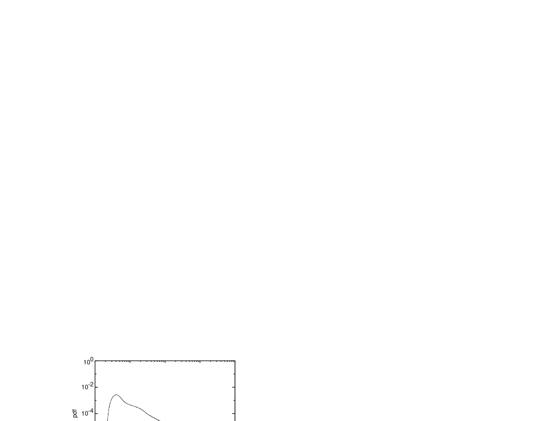
FIG. 11.: The pdf for the case where the pdf of $a_{t}$ has a level staircase structure at $a=2$, $\xi=2.5$, $p=0.95$, with $b_{t}=1$ ($10^{9}$ iterates, $10^{3}$ equispaced bins per unit of $\log X_{t}$).

TABLE III.: The first few $\mu=\mu_{R}+i\mu_{I}$ roots of (62, 64) and the predicted log-periodic frequencies for $a_{t}$ with a two level staircase distribution at $a=2$, $\xi=2.5$, and $p=0.95$.

$m$	1	2	3	4	5	6
$\mu_{R}(m)$	1.6535	2.4918	2.8418	3.0389	3.2015	3.3179
$\mu_{I}(m)$	0.0000	4.3475	8.0152	11.6794	15.3255	18.9598
$f(m)$	0.0000	1.5932	2.9373	4.2801	5.6163	6.9482

An important difference with the previous two-point pdf is that now the gap value is $\mu_{R}(2)-\mu_{R}(1)\simeq 0.84$, which is about three times larger than before. This means that the log-periodic structure are smaller and decay faster for large $X$. They are still quite visible as found in Fig. 11, where we can observe the undulation of $P(X)$’s tail. The results obtained for the various $b_{t}$ distributions (from a non-random $b_{t}=1$ to a uniform $b_{t}$ with $\beta=0$) are essentially the same for $X\geq 3$. The only difference is that a larger disorder in $b_{t}$ allows for an exploration of the interval closer to $0$. The Lomb power spectrum analysis is presented in Fig. 12. The fundamental frequency, $f(2)\approx 1.59$, is visible in all the simulations and more clearly in the spectral analysis where a strong peak appears in the Lomb power spectrum. The next higher frequency, $f(3)\approx 3.0$, is the only one which can be detected as the disorder in $b_{t}$ increases. All higher frequencies are lost in the noise. The reason for this is clear. The relative amplitude of a given frequency $f(m)$ is quantified by $\mu_{R}(m)-\mu_{R}(1)$. For the second frequency, we have $\mu_{R}(3)-\mu_{R}(1)=1.19$. For the third frequency, we have $\mu_{R}(4)-\mu_{R}(1)=1.39$ and so on. It seems that a difference $\mu_{R}(m)-\mu_{R}(1)$ of the order or less than $1$ is necessary for the clear detection of log-periodicity. Intuitively, this ensures that the amplitude of the oscillations does not decay more than by a factor $100$ over two decades. We notice that a similar gap about $1$ was found in the analysis of the log-periodic structure of DLA clusters [17]. The present analysis rationalizes why we have been able to detect these structures in this case.

FIG. 12.: (a) The Pdf tail for $a_{t}$ with two point distribution at $a=2$, $\xi=2.5$, $p=0.95$, and $b_{t}=1$ ($10^{9}$ iterates, $10^{3}$ equispaced bins per unit of $\log X_{t}$). (b) The logarithmic derivative of (a). (c) The Lomb periodogram of (b).

Table IV makes the comparison between the predicted and observed frequencies.

TABLE IV.: Predicted and observed frequencies for $a_{t}$ with a two level staircase distribution at $a=2$, $\xi=2.5$, $p=0.95$, and two different choices for $b_{t}$ distribution. The first row contains the predicted frequencies. Subsequent rows are the frequencies retrieved from the numerical simulations. The bold emphasis indicates the frequency that gives the largest peak in the spectrum. The other well-defined peaks are written in normal format, while numbers inside parenthesis correspond to peaks in the spectrum that are barely above the noise level of the Lomb periodgram.

$m$	1	2	3
$f(m+1)$	1.59	2.94	4.28
$f_{b_{t}=1}(m)$	$\bf{1.51}$	3.07	(4.31)
$f_{\beta=0}(m)$	$\bf{1.51}$	3.00	(4.50)

We conclude that a log-periodic structure of the tail of the $X_{t}$’s pdf is present for the smeared out two level staircase distribution, although its amplitude is weakened as compared to the previous two point distribution case. This was expected from the theoretical analysis of the influence of disorder [21, 17]. The important aspect of our result is that the log-periodicity, and the prefered scaling ratios $\lambda$, can no more be associated to a specifically chosen amplification factor, as for the previous two-point distribution. Notwithstanding the presence of a large disorder, a discrete set of effective scaling factors are selected. It is amazing to us how strong is this effect and how relatively weak is the influence of the disorder.

VI UNIFORM DISTRIBUTION

This last section deals with the effects of a very strong disorder on $a_{t}$. To attain this goal, we consider a uniform $a_{t}$-distribution

$$P_{a_{t}}(a_{t})={{\Theta(a_{t}-a_{\ell})-\Theta(a_{t}-a_{r}))}\over{a_{r}-a_{\ell}}}\;,$$ (65)

where

$$0 \leq a_{\ell}<1\;,$$ (66)

$$1 < a_{r}<\hat{a}_{r}(a_{\ell})\;.$$ (67)

$\hat{a}_{r}(a_{\ell})$ is such that (5) is obeyed and is the solution of

$$\hat{a}_{r}(a_{\ell})\ln\hat{a}_{r}(a_{\ell})-\hat{a}_{r}(a_{\ell})=a_{\ell}\ln a_{\ell}-a_{\ell}\;.$$ (68)

Figure 13 shows the allowed $a_{\ell}$–$a_{r}$ region.

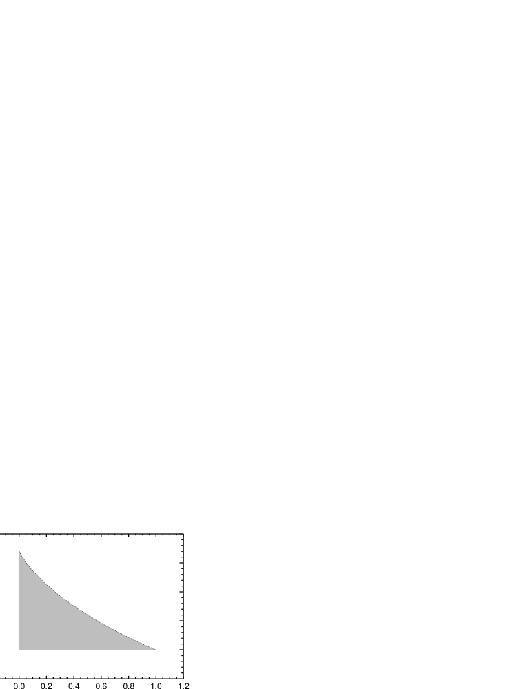
FIG. 13.: Allowed $a_{l}$–$a_{r}$ domain for $a_{t}$ with uniform distribution. The dotted boundary depicts the strict inequalities given in (67).

The largest width compatible with (5) corresponds to $a_{\ell}=0$ and $a_{r}=e$. When $a_{\ell}$ is made larger, the maximum value of $a_{r}$ progressively decays towards $1$.

The integral equation (17) is

$$P(X)={{1}\over{a_{r}-a_{\ell}}}\int_{a_{\ell}}^{a_{r}}{{P({X\over a_{t}})}\over a_{t}}da_{t}\;.$$ (69)

The tail of $P(X)$ takes the form of a power law if the exponent $\mu$ is the solution of

$$(\mu-1)(a_{r}-a_{\ell})=a_{r}^{\mu+1}-a_{\ell}^{\mu+1}\;.$$ (70)

With $\mu=\mu_{R}+i\mu_{I}$, we get

$$(\mu_{R}+1)(a_{r}-a_{\ell}) = a_{r}^{\mu_{R}+1}\cos({\mu_{I}\ln a_{r}})$$ (72)

$$\mbox{}-a_{\ell}^{\mu_{R}+1}\cos({\mu_{I}\ln a_{\ell}})\;,$$

$$\mu_{I}(a_{r}-a_{\ell}) = a_{r}^{\mu_{R}+1}\sin({\mu_{I}\ln a_{r}})$$ (74)

$$\mbox{}-a_{\ell}^{\mu_{R}+1}\sin({\mu_{I}\ln a_{\ell}})\;.$$

We select $a_{\ell}=0.001$ and $a_{r}=1.9$. The solutions with the smallest, positive, real parts are given in the table V, together with their corresponding log-frequencies $f$.

TABLE V.: The first few $\mu=\mu_{R}+i\mu_{I}$ roots of (72, 74) and the predicted log-periodic frequencies for the uniformly distributed $a_{t}$ with $a_{\ell}=0.001$ and $a_{r}=1.9$.

$m$	1	2	3	4	5
$\mu_{R}(m)$	1.2667	3.9414	4.8349	5.3984	5.8116
$\mu_{I}(m)$	0.0000	11.6095	21.6147	31.5024	41.3494
$f(m)$	0.0000	4.2545	7.9211	11.5446	15.1532

The most striking feature to note is the large gap value, $\mu_{R}(2)-\mu_{R}(1)\simeq 2.67$. These differences increase rapidly with the order $m$ of the solution. This implies that the oscillations must be extremely weak and severely dampened. In Fig. 14 we explore the dependence of the gap as a function of the parameters $a_{\ell}$ and $a_{r}$ of the model. If $a_{\ell}=0$ and $a_{r}=2.71$, we find $\mu_{R}(2)-\mu_{R}(1)\simeq 2.1$, but $\mu_{R}(1)=0.006$ is very small. When $a_{\ell}=0$ and $a_{r}=2.0$, we find $\mu_{R}(2)-\mu_{R}(1)=2.545$ with $\mu_{R}(1)=1.0$.

FIG. 14.: The gap value, $\mu_{R}(2)-\mu_{R}(1)$, as a function of $a_{r}$ for different choices of $a_{l}$.

The situation does not improve if we take $a_{\ell}\to 1^{-}$ and $a_{r}\to 1^{+}$ (while keeping the stationarity condition (5)). Notice that we need $a_{r}>1$ in order to get a solution for $\mu$, i.e to get a power law pdf for $X_{t}$. This stems from the fundamental fact that the power law pdf results from intermittent amplifications. In summary, the log-periodic oscillations are present theoretically but are very difficult to measure and quantify. The pdf for the $b_{t}=1$ case is shown in Fig. 15.

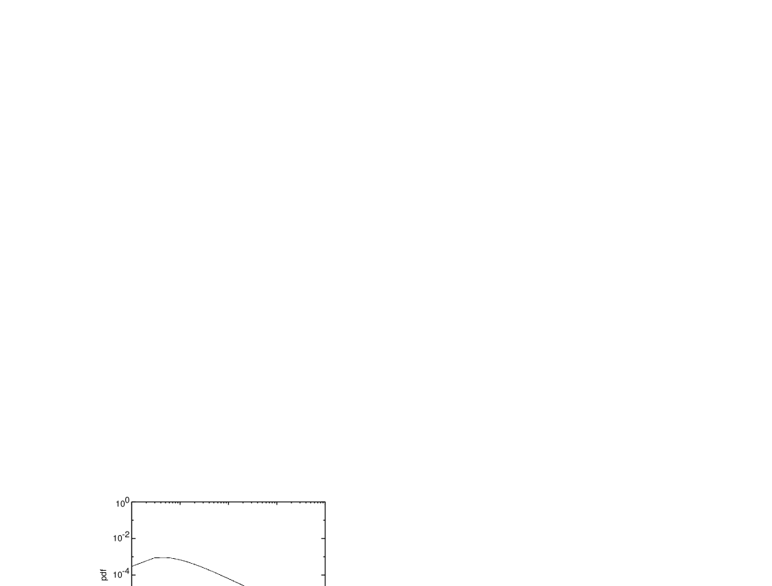
FIG. 15.: The pdf for $a_{t}$ with uniform distribution between $a_{l}=0.001$ and $a_{r}=1.9$; $b_{t}=1$ ($10^{9}$ iterates, $10^{3}$ equispaced bins per unit of $\log X_{t}$).

A segment of its tail is analyzed with the same procedure as was applied to the previous two $a_{t}$-distribution families (Fig. 16).

FIG. 16.: (a) The logarithmic derivative of the pdf of $X$ for $a_{t}$ with a uniform distribution between $a_{l}=0.001$ and $a_{r}=1.9$, $b_{t}=1$ ($10^{9}$ iterates, $10^{3}$ equispaced bins per unit of $\log X_{t}$). (b) The Lomb periodogram of (a).

Only $f(4)$ seems to be recognizable among all the peaks in the Lomb periodogram but this seems even far-fetched as the signal is within the noise level. In conclusion, this uniform case corresponds to a large gap and the log-periodic structures, that are present in theory, are not clearly visible.

VII CONCLUDING REMARKS

We started our analysis by considering the intermittent multiplicative processes of a simple binomial $a_{t}$ distribution. Not surprisingly, strong log-periodic corrections to the main power law probability density function have been found for the random affine map. The disorder in the additive constant smooths out the higher frequencies but does not dampen out the smallest log-periodic frequencies. We then analyzed situations with increasing disorder in the multiplicative terms. Instead of going to the weak disorder regime with two broadened peaks, we analyzed a pdf of multiplicative factors which consists of a two-step staircase. In this already large disorder regime, we have found that the log-periodic structure of the tail of the $X_{t}$’s pdf is present for the smeared out two level staircase distribution, although it is weakened in its amplitude as compared to the two point distribution case. The most important aspect of our results is that the log-periodicity, and the prefered scaling ratios $\lambda$, can no more be associated to a specifically chosen amplification factor, as for the two-point distribution. Notwithstanding the presence of a large disorder, a discrete set of effective scaling factors are selected. The “gap”, defined as the difference between the smallest exponent real part and the real solution, controls the strength of the log-periodicity. We have been able to determine that the gap must be of the order or less than $1$ in order for the log-periodicity to be strong. Larger gaps still lead to visible effects but the analysis must then be very precise and the noise level very low. This is the situation found for a uniform distribution of multiplicative factors. In summary, we have shown that log-periodicity remains a significant effect even in the presence of significant disorder.

VIII APPENDIX : DETERMINATION OF THE EXPONENTS FOR THE TWO-POINT DISTRIBUTION USING A PERTURBATIVE ANALYSIS

The power law structure of the $P(X)$ pdf characterizes rare excursions of $X_{t}$ to large values. These large values are reached by repeated occurrence of the amplifying multiplicative factor $a^{\xi}$. This motivates us to make the approximation of neglecting the first “damping” term in the r.h.s. of (37),

$$P(X)\approx(1-p)a^{-\xi}P(a^{-\xi}X)\;.$$ (75)

This functional equation is simpler to handle. It also has a form reminiscent of the renormalization group equation that Feigenbaum used in his analysis of a bifurcation sequence of the logistic equation [47]. Analoguous equations has also been discussed in [11, 12, 13, 21]. Assuming a power law form for $P(X)$ ($P(X)={A\over X^{1+\mu}}$) provides for the $\mu$ equation :

$$(1-p)a^{\mu\xi}=1\;.$$ (76)

With the notation $z=e^{x+iy}=a^{\mu_{R}+i\mu_{I}}$, we obtain

$$x = -{{1}\over{\xi}}\ln(1-p)\quad\mbox{and}\quad\mu_{R}=-{{\ln(1-p)}\over{\xi\ln a}}$$ (77)

$$y = {{2k\pi}\over{\xi}}\quad\mbox{and}\quad\mu_{I}={{2\pi}\over{\ln\lambda_{k}}}\;,$$ (79)

$$\mbox{}\quad\mbox{where}\quad\lambda_{k}\equiv a^{\xi/k},\quad k\quad\mbox{ integer}\;.$$

An approximation of the imaginary part of the roots of (46) therefore is

$$y={2k\pi\over\xi}\;.$$ (80)

This agrees fairly well with the exact computed roots shown in table I. We can improve on this estimation by inserting the parametrization

$$y={2k\pi\over\xi}+\epsilon\;,$$ (81)

in the full set of equations (48) and (50). This yields the following system of two equations of the two unknown $x$ and $\epsilon$ :

$$((1-p)e^{(1+\xi)x}\cos\epsilon(1+\xi)-e^{x}\cos\epsilon)\cos{{2k\pi}\over\xi}$$ (82)

$$\mbox{ }-((1-p)e^{(1+\xi)x}\sin\epsilon(1+\xi)$$ (83)

$$\mbox{\hskip 28.45274pt}\;\;-e^{x}\sin\epsilon)\sin{{2k\pi}\over\xi}+p=0\;,$$ (84)

$$((1-p)e^{\xi x}\cos\epsilon(1+\xi)-\cos\epsilon)\sin{{2k\pi}\over\xi}$$ (85)

$$\mbox{ }\;\;+((1-p)e^{\xi x}\sin\epsilon(1+\xi)$$ (86)

$$\mbox{\hskip 28.45274pt}-\sin\epsilon)\cos{{2k\pi}\over\xi}=0\;.$$ (87)

Assuming $\epsilon(1+\xi)$ to be “small”, we expand the trigonometric functions to first order in $\epsilon$ :

$$( (1-p)e^{(1+\xi)x}-e^{x})\cos{2k\pi/\xi}-\epsilon((1-p)(1+\xi)e^{(1+\xi)x}$$ (89)

$$\mbox{\hskip 28.45274pt}-e^{x})\sin{2k\pi/\xi}+p=0\;,$$

$$( (1-p)e^{\xi x}-1)\sin{2k\pi/\xi}+\epsilon((1-p)(1+\xi)e^{\xi x}$$ (91)

$$\mbox{\hskip 28.45274pt}-1)\cos{2k\pi/\xi}=0\;.$$

Eliminating $\epsilon$ between the two preceding equations, we get an equation in the sole variable $x$ :

$$(1-p)e^{(1+\xi)x}-e^{x}+p\cos{2k\pi/\xi}=0\;.$$ (92)

There is a unique solution in $x$ for each $k$. Knowing $x$, we then get $\epsilon$ from

$$\epsilon=-{{(1-p)e^{\xi x}-1}\over{(1-p)(1+\xi)e^{\xi x}-1}}\,\tan{2k\pi\over\xi}\;.$$ (93)

Table VI compares these solutions to the exact ones, in the case when $a=2$, $\xi=2.5$, $p=0.95$.

TABLE VI.: The appoximate (according to (92, 93, 81)) and the exact (from (48, 50)) roots for $a_{t}$ with two point distribution at $a=2$, $\xi=2.5$, and $p=0.95$.

$k$	0	1	2	3	4	5
$x_{apprx}(k)$	1.0333	1.2760	1.1597	1.1597	1.2760	1.0333
$x_{exact}(k)$	1.0333	1.2808	1.1922	1.1922	1.2808	1.0333
$\epsilon(k)$	0.0000	0.0480	-0.1301	0.1301	-0.0480	0.0000
$y_{apprx}(k)$	0.0000	2.5612	4.8965	7.6699	10.0051	12.5664
$y_{exact}(k)$	0.0000	2.5605	4.9101	7.6563	10.0058	12.5664

REFERENCES

- [1] Bessis D., J.S. Geronimo and P. Moussa, J. Physique-Lett. 44, L977 (1983).
- [2] B. Derrida, C. Itzykson and J.M. Luck, Commun. Math. Phys. 94, 115 (1984).
- [3] Douçot B., W. Wang, J. Chaussy, B. Pannetier and R. Rammal, Phys. Rev. Lett. 57, 1235 (1986).
- [4] D. Bessis, J.-D. Fournier, G. Servizi, G. Tourchetti and S. Vaienti, Phys. Rev. A 36, 920 (1987); J.-D. Fournier, G. Tourchetti and S. Vaienti, Phys. Lett. A 140, 331 (1989).
- [5] M.O. Vlad and M.C. Mackey, Physica Scripta 50, 615 (1994).
- [6] Y. Meurice, G. Ordaz, V.G.J. Rodgers, Phys. Rev. Lett. 75, 4555 (1995).
- [7] W.I. Newman, D.L. Turcotte and A.M. Gabrielov, Phys. Rev. E 52, 4827 (1995).
- [8] B. Kutjnak-Urbanc, Stefano Zapperi, S. Milošević and H. E. Stanley, Phys. Rev. E 54, 272 (1996).
- [9] Schlesinger M.F. and B.J. West, Phys. Rev. Lett. 67, 2106 (1991).
- [10] B.J. West, Int. J. Mod. Phys. B 4, 1629 (1990); Annals of Biomedical Engineering, 18, 135 (1990); B.J. West and W. Deering, Phys. Rep. 246, 1 (1994).
- [11] J.-C. Anifrani, C. Le Floc’h, D. Sornette and B. Souillard, J. Phys. I (France) 5, 631 (1995).
- [12] D. Sornette and C.G. Sammis, J. Phys. I (France) 5, 607 (1995).
- [13] H. Saleur, C.G. Sammis and D. Sornette, J. Geophys. Res. 101, 17661 (1996).
- [14] A. Johansen, D. Sornette, H. Wakita, U. Tsunogai, W.I. Newman and H. Saleur, J. Phys. I (France) 6, 1391 (1996).
- [15] D.J. Varnes and C.G. Bufe, Geophys. J. Int. 124, 149 (1996).
- [16] G. Ouillon, D. Sornette, A. Genter and C. Castaing, J. Phys. I (France) 6, 1127 (1996).
- [17] D. Sornette, A. Johansen, A. Arnéodo, J.-F. Muzy and H. Saleur, Phys. Rev. Lett. 76, 251 (1996).
- [18] Y. Huang, G. Ouillon, H. Saleur and D. Sornette, Phys. Rev. E, in press (1997).
- [19] D. Sornette, A. Johansen and J.-P. Bouchaud, J. Phys. I (France) 6, 167 (1996); D. Sornette and A. Johansen, Physica A, in press (http://xxx.lanl.gov/cond-mat/9704127) (1997).
- [20] Feigenbaum, J.A., and P.G.O. Freund, Int. J. Mod. Phys. 10, 3737 (1996).
- [21] H. Saleur and D. Sornette, J. Phys. I (France) 6, 327 (1996).
- [22] D. J. Wallace, R. K. P. Zia, Phys. Lett. A 48, 325 (1974).
- [23] J.-H. Chen and T.C. Lubensky, Phys. Rev. B 16, 2106 (1977).
- [24] Aharony A., Phys. Rev. B 12, 1049 (1975).
- [25] D.E. Khmelnitskii, Phys. Lett. A 67, 59 (1978).
- [26] Boyanovsky D. and J.L. Cardy, Phys. Rev. B 26, 154 (1982).
- [27] A. Weinrib and B.I. Halperin, Phys. Rev. B 27, 413 (1983).
- [28] D. Sornette, Discrete scale invariance and complex exponents, Physics Reports (submitted) (http://xxx.lanl.gov/abs/cond-mat/9707012)(1997).
- [29] Bernasconi J. and W.R. Schneider, J. Phys. A 15, L729 (1983).
- [30] M.O. Vlad, Int. J. Mod. Phys. B 6, 417 (1992); M.O. Vlad, J. Phys. A 25, 749 (1992).
- [31] C. de Calan, J.-M. Luck, Th. M. Nieuwenhuizen and D. Petritis, J. Phys. A 18, 501, (1985).
- [32] L. de Haan, S.I. Resnick, H. Rootzén and C.G. de Vries, Stochastic Processes and their Applications 32, 213, (1989).
- [33] H. Kesten, Acta Math. 131, 207, (1973).
- [34] D. Sornette and R. Cont, J. Phys. I (France) 7, 431 (1997).
- [35] M. Levy and S. Solomon, Int. J. Mod. Phys. C 7, 595 (1996); Int. J. Mod. Phys. C 7, 745 (1996).
- [36] D. Sornette and L. Knopoff, preprint (1997)
- [37] G. Hughes and J.L.G. Andújar, Nature 387, 241 (1997).
- [38] W.H. Greene, Econometric Analysis, 2nd ed. (Prentice Hall, Engelwood Cliffs, NJ, 1992).
- [39] H.L. Yang and Z.Q. Huang, Phys. Rev. Lett. 77, 4899 (1996).
- [40] A. Crisanti, G. Paladin and A. Vulpiani, Products of random matrices in statistical physics (Springer Verlag, Berlin, 1993).
- [41] F.R. Gantmacher, The Theory of Matrices (Chelsea Publishing Company, New York, 1959).
- [42] U.M.S. Costa, M.L. Lyra, A.R. Plastino and C. Tsallis, (http://xxx.lanl.gov/cond-mat/9701096) (1997).
- [43] M. Blank, Discreteness and continuity in problems of chaotic dynamics (Amer. Math. Soc., Providence, RI, 1997).
- [44] L. Biferale, M. Blank, and U. Frisch, J. Stat. Phys. 75, 781 (1994).
- [45] M.F. Barnsley, The science of fractal images, ed. by H.O. Peitgen and D. Saupe (Springer Verlag, Heidelberg, 1988).
- [46] W.H. Press, S.A. Teukolsky, W.T. Vetterling and B.P. Flannery, Numerical Recipes (Cambridge University Press, Cambridge, UK, 1992).
- [47] M.J. Feigenbaum, J. Stat. Phys. 19, 25 (1978); 21, 669 (1979); P. Coullet and C. Tresser, J. Phys. Coll. 39, C5 (1978); C. R. Acad. Sci. 287, 577 (1978); P. Collet and J.P. Eckmann, Iterated maps of the interval and dynamical systems (Birkhauser, Boston, 1980)