Modeling sublimation by computer simulation:
morphology dependent effective energies

Abstract

Solid-On-Solid (SOS) computer simulations are employed to investigate the sublimation of surfaces. We distinguish three sublimation regimes: layer-by-layer sublimation, free step flow and hindered step flow. The sublimation regime is selected by the morphology i.e. the terrace width. To each regime corresponds another effective energy. We propose a systematic way to derive microscopic parameters from effective energies and apply this microscopical analysis to the layer-by-layer and the free step flow regime. We adopt analytical calculations from Pimpinelli and Villain and apply them to our model.

keywords: Computer simulations; Models of surface kinetics; Evaporation and Sublimation; Growth; Surface Diffusion; Surface structure, morphology, roughness, and topography; Cadmium telluride
PACS: 81.10.Aj; 68.35.Fx; 68.10.Jy

1 Introduction

The sublimation of semiconductor materials such as cadmium telluride or silicium has been of considerable interest in the last few years. The motivation of these studies has been mainly to understand the kinetics on these surfaces. This would be helpful e.g. to gain better control in the fabrication of nanostructure devices. In this paper we want to describe computer simulations of sublimation. We use the conceptually simple SOS model which has been extensively used to model Molecular Beam Epitaxy (MBE) [1, 2]. As far as we know these are the first simulations of sublimation of this kind.

Theoretical studies of sublimation were based on the 1+1 dimensional Burton-Cabrera-Frank model. In this model the evolution of the surface is described by the motion of steps. In 2+1 dimensions it can be interpreted as a surface of parallel, mono-atomic and straight steps. Pagonabarraga et. al. examined the validity of the continuum approximation in the step flow regime [3]. Pimpinelli and Villain discussed the creation of surface vacancies and found a condition for the occurrence of “Lochkeime” (poly-vacancies) [4]. In the following we will refer to calculations in their introductory book of crystal growth [5]. In particular they found that in step flow sublimation the velocity of steps is influenced by the terrace width.

Experimental studies of CdTe(001) concentrated on the extraction of effective energies. Several authors used Reflection High Energy Electron Diffraction (RHEED) to study sublimation [6, 7, 8]. Other investigations were based on the use of a quadrupole mass spectrometer (QMS) [9, 10] (and references therein). Recently Neureiter et al applied Spot Profile Analysis of Low Energy Electron Diffraction (SPA-LEED) to CdTe(001)[11, 9]. The oscillation period $\tau$ in RHEED or SPA-LEED intensity can be described by an arrhenius-law $1/\tau=\nu\;\mbox{e}^{-E/kT}$. For CdTe(001) an activation energy of $1.9eV$ - derived from the diffraction data - is commonly accepted . Using QMS a value of $1.55eV$ for the mass desorption rate has been reported. We will show that this discrepancy can be explained by the existence of different morphology dependent sublimation regimes. Neureiter et. al. show that such a picture of the CdTe(001) surface is consistent with SPA-LEED and QMS measurements[9].

It would be desirable to obtain microscopic parameters of a computer model from ab-initio calculations. Calculations are now available for GaAs(001) [12, 13], but for II-VI semiconductors no such calculations are available yet. Thous computer simulations of MBE or sublimation can help to get insight into these parameters. E.g. Šmilauer and Vvedensky were able to find a set of parameters for GaAs(001). They compared the step density of their model to RHEED intensities during MBE growth and subsequent recovery [14]. These investigations showed that it is possible to describe such a complicated surface (reconstruction, 2 types of atoms …) by means of the simplest SOS model. Naturally the microscopic parameters found are still effective parameters. We expect that these values should be related to the true microscopic interactions describing the slowest processes.

There is a certain advantage in using sublimation data compared to MBE to find microscopic parameters of real materials. First of all the process is determined uniquely by microscopic processes, whereas in MBE the evolution of the morphology is dominated by the external flux of atoms. Secondly, sublimation has been recently studied by SPA-LEED [11, 9]. To a great extent this method can be analyzed in kinematic approximation [15, 16], whereas RHEED-profiles have to be calculated using multiple-scattering theory [17]. Also the mass desorption during sublimation can be easily compared with computer simulations.

The organization of this paper is as follows. In section two we will introduce the SOS model and the algorithm used in the simulations. In section three we will investigate sublimation similar to experimental investigations. We will identify three sublimation regimes in dependence of the terrace width. In section four we will connect effective activation energies (which are measurable in real experiments) to the underlying microscopic parameters. On the one hand we will be able to compare these relations with theoretical predictions of Pimpinelli and Villain (section five). On the other hand this leads to a systematic approach for determining microscopic energies of real materials which will be illustrated in section six. A discussion and an outlook will follow in section seven.

2 Solid-On-Solid model

One basic assumption in this model is the neglection of overhangs. Thus no bulk vacancy formation can be investigated. The second assumption is a fixed lattice structure. Both lead to the crucial simplification for the simulation that the surface can be stored in one simple data-array of heights.

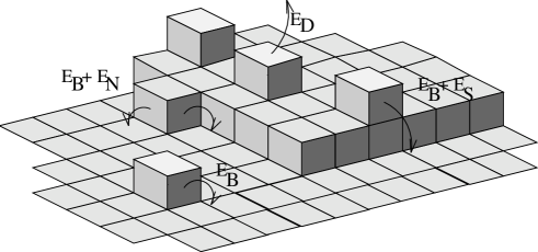
Figure 1: The activation energy in the jump rate of atoms depends on the local arrangement. The diffusion barrier is $E_{B}$, for desorption an energy of $E_{D}$ is necessary. Next in-plane neighbours have a binding energy of $E_{N}$. A jump over a step edge is hindered by the Ehrlich-Schwoebel barrier $E_{S}$.

We have used a simple version of this model: a simple cubic lattice with only one species of atoms. Since there is only one lattice constant all lengths will be given in units of this lattice constant. Figure 1 shows some selected processes and their corresponding activation energies.

Theories of activated processes lead to an arrhenius form of the jump frequency $\Gamma=\nu_{0}\>\mbox{e}^{-E/kT}$ [18]. The prefactor in general depends on the form of the potential and the temperature. Nevertheless the exponential factor gives the dominant temperature dependence. Thus we assume a constant prefactor $\nu_{0}$. The activation energy depends on the microscopic mechanism involved. We assume that diffusion has an activation energy of $E=E_{B}+n\cdot E_{N}$ where $n$ is the number of next in-plane neighbours. Thus free atoms in this model have the diffusion constant $D=\nu_{0}\>\mbox{e}^{-E_{B}/kT}$. At step edges an Ehrlich-Schwoebel barrier $E_{S}$ is considered. In addition to “conventional” SOS-models of MBE we take into account the desorption similar to the diffusion with an jump frequency $\Gamma_{desorption}=\nu_{0}\>\mbox{e}^{-(E_{D}+n\cdot E_{N})/kT}$. We assume the same prefactor for desorption as for diffusion which is certainly not valid in real materials.

Especially when simulating sublimation it is absolutely important to include all possible events because even events with very low rates can become very important. E.g. the creation of a surface vacancy has a rate which is several orders of magnitudes lower then the jump frequency of free adatoms. Nevertheless this process is the most important one to initiate layer-by-layer sublimation.

The Maksym-algorithm [19] is able to handle such big differences in jump rates. In this algorithm all possible events are considered simultaneously and are stored in one array of rates. The event with a high rate will be chosen with a corresponding high probability. Maksym described how to find in an efficient way the event selected by a random number in the range $(0,\sum rates)$. We improved the simulation of the (time consuming) diffusion of free adatoms by handling them separately.

In this paper we will concentrate on two sets of parameters: $\nu_{0}=10^{12}s^{-1},\>\>E_{B}=0.9eV,\>\>E_{D}=1.1eV,\>\>E_{N}=0.25eV,\>\mbox{ and }\>E_{S}=0.1eV$ (set 1). A second set $\nu_{0}=10^{12}s^{-1},\>\>E_{B}=0.5eV,\>\>E_{D}=0.7eV,\>\>E_{N}=0.35eV,\>\mbox{ and }\>E_{S}=0.1eV$ (set 2) will be compared.

3 Crossover from layer-by-layer to step flow sublimation

Since computer simulations are restricted to rather small systems (we use system sizes up to $800\times 800$ lattice constants, typically $512\times 512$), one is forced to induce equidistant steps by fixing a height difference between two opposite boundaries. We have investigated the effect of such an induced step train on the mass desorption.

There are two limiting cases. First the pure layer-by-layer sublimation. In this case the poly-vacancies are much smaller then typical terrace sizes. Changing the terrace sizes in this regime should not influence the total amount of layers desorbed after a fixed time. Furthermore the number of layers desorbed should be equal to the number of periods observed in LEED or RHEED.

In the second extreme the steps are so close together that there is no place to create poly-vacancies and there will be only desorption from steps. In this case the number of desorbed monolayers $\Delta h$ after the time $\Delta t$ will be equal to

$$\frac{\Delta h}{\Delta t}=\frac{v_{step}}{L_{terrace}}$$

because $L_{terrace}/v_{step}$ is just the time to evaporate one monolayer.

Figure 2: Height loss per time over $1/L_{terrace}$. Each data point represents a simulation of parameter set (1) at $600K$. For all simulations $\Delta t$ was chosen to be $800s$. The dashed line corresponds to $v_{step}=0.154s^{-1}$.

Figure 2 clearly show the existence of these two regimes. However at very small terrace sizes a third regime can be identified (we have not plotted another data point at $1/L_{terrace}=0.2$ which clearly establishes region III). This behaviour was already calculated by Pimpinelli and Villain using the modified Burton-Cabrera-Frank (BCF) model[5]. In this framework but without a Schwoebel-effect (however the estimation is valid in general) $v_{step}\propto\tanh(L_{terrace}/2\sqrt{D\tau_{D}})$, where $D$ is the diffusion constant of free atoms and $\tau_{D}$ the life-time of an particle until desorption occurs. If the terrace width is greater then the diffusion length $\sqrt{D\tau_{D}}$ one gets a constant velocity. But if one lowers $L_{terrace}$ the particles will cross the terraces and will be reincorporated at the step edges. In this case $v_{step}$ will be proportional to $L_{terrace}$ and $\Delta h/\Delta t$ will become constant again. That is why we want to distinguish between hindered and free step flow. Setting the argument of the tanh to one and identifying $D=\nu_{0}\;\mbox{e}^{-E_{B}/kT}\mbox{ and }1/\tau_{D}=\nu_{0}\;\mbox{e}^{-E_{D}/kT}$ one can estimate the crossover length between regime II and III to be $\ell_{\times}\approx 14$ in good correspondence to figure 2.

Likewise Pimpinelli and Villain calculated the crossover between the free step flow and the layer-by-layer regime. In the approximation described in section five we obtain for parameter set (1) a crossover length of about 60, which is once again in good correspondence to our simulations. However we will show in section five that this agreement of theory and simulation is merely by chance.

In addition we have investigated the intensity in antiphase of the (0,0)-spot using the kinematic approximation. We found that the oscillation period was the same either by calculating the step density or the width of the height distribution (in the case of singular surfaces). The evaluation of the LEED-profiles is complicated by the fact that due to the small system sizes the distribution of terrace sizes is limited. This leads to a pronounced twin-peak structure in k-space at $k_{peak}=\pm\frac{2\pi}{L_{terrace}}$. We have mimicked the effect of a broad distribution of terrace sizes by convolution of the obtained profile with an Gaussian of $0.5\%$ of the Brioullin Zone. In correspondence to the conclusions drawn from the mass desorption diagram (fig. 2) one oscillation period of $232s\pm 8$ down to a terrace size of $L_{terrace}\approx 100$ is observed. At $L_{terrace}=64$ an oscillation could be identified in the twin peak structure. However the period could only be estimated to be roughly $\tau\approx 265s\pm 20s$. With $L_{terrace}=32$ no such oscillations occurred.

We have shown that in regime I (layer-by-layer sublimation) the observed oscillations are independent of the terrace size. Decreasing the mean terrace width one reaches the free step flow regime (regime II) which is characterized by a constant step velocity. Furthermore oscillations do not exist in this regime. However at small terrace sizes (small compared to the diffusion length) one reaches the hindered step flow regime III which is again characterized by a mass desorption rate independent of the terrace width.

Figure 3: Comparison of the activation energies of the layer-by-layer and the free step flow sublimation of parameter set (1). In the layer-by-layer regime ($L_{terrace}=256$) the oscillation period is characterized by the effective activation energy $E_{I}=1.73eV$. At $L_{terrace}=16$ the step velocity yields $E_{II}=1.60eV$.

In each regime one could expect to define effective energies. In regime I the oscillation period is a well defined variable. In regime II -the free step flow regime- the step velocity and at small terrace sizes (regime III) the mass desorption rate can be analyzed. We concentrate on regime I and II but we will mention the theoretical result (including the Ehrlich-Schwoebel-barrier) in section 5.3 for regime III. Looking at the temperature dependence of $1/\tau$ and $v_{step}$ (figure 3) one can indeed identify arrhenius laws with different activation energies.

4 Interpretation of effective energies: microscopical analysis

We will now try to establish a link between the microscopic parameters of the model to the effective energies. The effective energies are derived from the variation of the temperature. In the simulations however it is possible to vary the microscopic parameters as well.

We will vary the energies of set (1) by fixing three energies and changing the fourth. In detail we have set the parameters to $E_{B}/eV$={0.8, 0.85, 0.9, 0.95}, $E_{D}/eV$={1.00, 1.05, 1.10, 1.15}, $E_{N}/eV$={0.23, 0.24, 0.25, 0.26} and $E_{S}/eV$={0.05, 0.10, 0.15, 0.20}. Assuming a linear dependence of the effective energy on the parameters $E_{\mbox{\small\tt regime}}=\beta E_{B}+\delta E_{D}+\nu E_{N}+\sigma E_{S}$ we want to extract the importance of the different microscopic parameters.

4.1 Layer-by-layer sublimation (regime I)

Our simulations at different temperatures (s. figure 3 ) show an arrhenius behaviour with $\nu^{T}_{I}=1.48\;10^{12}\;s^{-1}$ and an effective activation energy of $E^{T}_{I}=1.73\;eV$. The upper index “T” indicates that these are values obtained by simulations at different temperatures.

The investigation of the effect of the microscopic parameters yields $\nu^{l.a.}_{I}=6.3\;10^{11}\;s^{-1}$ and

$$E^{l.a.}_{I}=0.61\cdot E_{B}+0.35\cdot E_{D}+2.85\cdot E_{N}+0.44\cdot E_{S}.$$

In our case this leads to an effective activation energy close to the “conventional” effective energy

$$E^{l.a.}_{I}=1.69eV\approx E^{T}_{I}=1.73eV.$$

Note that $E^{l.a.}_{I}$ has been deduced from simulations at a fixed temperature $T=600K$. At first glance it is surprising that the diffusion parameter $E_{B}$ has a larger influence on the effective energy than the desorption energy $E_{D}$. This can be explained by the typical life of an evaporating particle. Firstly the atoms become freely diffusing atoms (this needs an activation energy of typically $E_{B}+3\cdot E_{N}$. Thereafter the atoms diffuse on the terrace until they evaporate. The Ehrlich-Schwoebel barrier plays an essential role in the creation of surface vacancies which explains the influence of $E_{S}$.

Figure 4: Temperature dependent sublimation rate in the layer-by-layer regime of set (2). However the predicted curve was multiplied by a factor 1.2 to show that the predicted energy is very good.

$E_{B}/eV$	$E_{D}/eV$	$E_{N}/eV$	$E_{S}/eV$	$\tau_{period}/s$	$\tau_{predicted}/s$
0.82	1.20	0.16	0.2	9.2	3.2
0.50	0.70	0.35	0.1	28	37
0.75	0.80	0.30	0.1	89	88
0.42	0.42	0.42	0.1	122	103
1.15	1.30	0.20	0.1	1290	1181

Table 1: Predicted and measured Oscillation periods. The simulations were carried out at $T=600K$, the vibration frequency was set to $\nu_{0}=12^{12}s^{-1}$

Other simulations show, that this approximation of first order is valid over a greater range in parameter space. The predicted periods of these models are compared with measured ones in Table 1. Figure 4 shows that the activation energy predicted by our linear approximation is still very good for the set (2) although the prefactor no longer holds.

4.2 Free step flow (regime II)

In the following investigations we used a surface with a mean terrace size of 16 lattice constants. Looking at Figure 2 one can see that one is in the free step flow regime.

By evaluating the temperature dependence in this extreme limit we find $\nu_{II}^{T}=3.9\cdot 10^{12}\;s^{-1}$ and $E_{II}^{T}=1.60eV$.

As in the case of layer-by-layer sublimation we connected this effective relation to the microscopic parameters. Of course we cannot be sure to stay in the free step flow regime. We checked that $\Delta h/\Delta t$ is at least twice as high as in the pure layer-by-layer regime. However with high $E_{D}$ or low $E_{B}$ we reached the hindered step flow regime due to the fact that the atoms stayed to short a time on the terrace.

Our results can be fitted by

$$E_{II}^{l.a.}=0.70\cdot E_{B}+0.32\cdot E_{D}+2.4\cdot E_{N}+0.21\cdot E_{S}$$

In this case the two different effective energies are identical $E^{l.a}_{II}=E^{T}_{II}=1.60eV$. Likewise the prefactor of $4.3\cdot 10^{12}\;s^{-1}$ is close to the previous one.

Comparing this relation with the equivalent relation for the layer-by-layer regime one observe that the contribution of $E_{N}$ and $E_{S}$ have significantly changed. This seems plausible because the creation of a surface vacancy compared to the creation of a kink is hindered by the energy $E_{N}+E_{S}$.

Figure 5: Predictions and measurements of $v_{step}$ for parameter set (2). No corrections were necessary!

A comparison between our prediction for the set (2) and measurements are shown in figure 5. As one can see our linear approximation is very good in this case.

5 Comparison with theoretical calculations

Now we are able to compare the theoretical predictions of Villain and Pimpinelli with our results. We will interpret variables in their results in terms of arrhenius activated jump rates.

5.1 Free step flow (regime II)

In the free step flow regime they obtained the following expression for $v_{step}$ on a surface with terraces of equal size $\ell$ (ch. 6.4 in [5])

$$v_{step}=\rho_{0}\kappa D\frac{4-\left(2-\kappa D\left(\frac{1}{D^{\prime\prime}}+\frac{1}{D^{\prime}}\right)\right)\mbox{e}^{-\kappa\ell}-\left(2+\kappa D\left(\frac{1}{D^{\prime\prime}}+\frac{1}{D^{\prime}}\right)\right)\mbox{e}^{\kappa\ell}}{\left(1+\kappa\frac{D}{D^{\prime}}\right)\left(1+\kappa\frac{D}{D^{\prime\prime}}\right)\mbox{e}^{\kappa\ell}-\left(1-\kappa\frac{D}{D^{\prime}}\right)\left(1-\kappa\frac{D}{D^{\prime\prime}}\right)\mbox{e}^{-\kappa\ell}}.$$

$\rho_{0}$ can be identified with the ratio between the detachment rate from a step and the diffusion jump rate ($\rho_{0}=\mbox{e}^{-(n\cdot E_{N})/kT}$, where $n\cdot E_{N}$ is a typical binding-energy to next in-plane neighbours at a step). The diffusion parameters at step edges are related with the diffusion constant $D$. Diffusion downward a step $D^{\prime}=\mbox{e}^{-E_{S}/kT}D$. Diffusion towards a step from the lower terrace is not changed in our model ($D^{\prime\prime}=D=\nu_{0}\cdot\mbox{e}^{-E_{B}/kT}$) . The inverse of the diffusion length is given by $\kappa=1/\sqrt{D\tau_{D}}=\mbox{e}^{-(E_{D}-E_{B})/2kT}$. Taking the limit for $\kappa\ell\gg 1$ (free step flow) and neglecting $\mbox{e}^{-(E_{D}-E_{B})/kT}$ versus 1 we obtain the simpler relation

$$v_{step}\approx\nu_{0}\mbox{e}^{-\frac{E_{B}/2+E_{D}/2+n\cdot E_{N}}{kT}}\cdot\left(1+\frac{1}{1+\mbox{e}^{-(E_{D}/2-E_{B}/2-E_{S})/kT}}\right).$$

This shows that the assumption of an arrhenius behaviour is not valid in this sublimation regime. However with parameter set (1) the correction factor has no temperature dependence . Because $E_{D}/2-E_{B}/2=E_{S}$ we obtain $v_{step}\approx 3/2\>\nu_{0}\mbox{e}^{-(E_{B}/2+E_{D}/2+n\cdot E_{N})/kT}$. In the microscopical analysis we measure an effective importance of $E_{D}$, $E_{B}$ and $E_{S}$ due the correction factor. The influence of $E_{N}$ is unchanged. Indeed if we use the theoretical result with $n\cdot E_{n}=2.4\cdot E_{N}$ (as the microscopical analysis suggests) we obtain an effective energy of $1.6eV$ in correspondence to our measurement.

5.2 Crossover to layer-by-layer sublimation

Given the two equations for the period of oscillations and the step velocity we can calculate in our linear approximation approach the dependence of $L_{\times}$ from the temperature and the microscopic parameters. From $1/\tau=v_{step}/L_{\times}$ we obtain

$$L_{\times}=\frac{\nu_{fsf}}{\nu_{lbl}}\mbox{e}^{-(E_{fsf}-E_{lbl})/kT}\approx 6.8\mbox{e}^{(0.03E_{D}-0.09E_{B}+0.45E_{N}+0.23E_{S})/kT}.$$

We already mentioned the theoretical relation for the crossover terrace width. Pimpinelli and Villain estimated the crossover to be at

$$\ell_{\times}^{2}\ln\ell_{\times}\approx 4\pi\left(\frac{\gamma}{kT}\right)^{2}\tau_{D}D\left(1+\frac{\Lambda\sigma_{0}}{D\rho_{0}}\right).$$

$\sigma_{0}$ is the equilibrium concentration and $\Lambda$ the diffusion constant of the surface vacancies. $\gamma$ is the free energy per step length. Neglecting $\Lambda$ and setting $\gamma=E_{N}$ (which is a good approximation if the step is nearly free of kinks) we can relate this expression to our model. If we simplify their relation in the vicinity of $\ell_{\times}$ at $T=600K$ we obtain approximately

$$\ell_{\times}\approx\sqrt{\pi}\left(\frac{E_{N}}{kT}\right)\cdot e^{(E_{D}-E_{B})/kT}.$$

which is at the same order of magnitude as our result but has a very different temperature dependence. In the theoretical result only desorption and diffusion energies contribute to the exponential temperature dependence. Whereas our simulations indicate that these terms cancel out and only $E_{N}$ and $E_{S}$ contribute exponentially.

5.3 Hindered step flow (regime III)

We have not examined in detail the hindered step flow regime by computer simulations. Nevertheless we want to mention the theoretical result for this regime. In this regime $\kappa\ell\ll 1$ and therefor one can use the Taylor series of the exponential functions $\mbox{e}^{\pm\kappa\ell}\approx 1\pm\kappa\ell$. In this case the step velocity is described by an arrhenius behaviour.

$$v_{step}\approx\ell\nu_{0}\mbox{e}^{-(E_{D}+n\cdot E_{N})/kT}$$

This means that the number of monolayers desorbed is independent of the terrace width in this regime.

6 Systematic derivation of microscopic energies

Our connection between effective and microscopic energies will help to develop a set of parameters describing e.g. the CdTe(001) surface. Taking the effective energies for CdTe(001) as $E_{I}=1.9eV$ and $E_{II}=1.55eV$ we can then reduce the four dimensional energy-parameter space to a two dimensional one. E. g. the Schwoebel-barrier can be expressed in terms of the diffusion and desorption barriers: $E_{S}=0.31eV+1.16E_{B}+0.16E_{D}$. In figure 6 the $E_{N}(E_{B},E_{D})$-plane is shown. But because there are further physical restrictions (namely that $E_{B}>0$, $E_{N}>0$ and $E_{D}>E_{B}$) only a triangle is left from the infinite plane. One should however be careful. In the dark region (where $E_{D}<E_{B}+E_{S}$) surface vacancies will be created via direct desorption rather than the creation of an adatom-vacancy pair. In this region our microscopic analysis is certainly incorrect. It should be emphasized that our relation of effective to microscopic energies is only valid in the vicinity of parameter set (1). However one can take it as a first approximation. Then one can systematically improve the result by iterating the microscopic analysis.

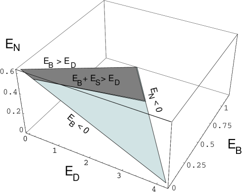
Figure 6: Proposed parameter plane $E_{N}(E_{B},E_{D})$ for CdTe(001). Due to physical constraints a triangle is cut out. In the dark region our microscopical analysis is not valid. There the process of the generation of surface vacancies is changed.

7 Conclusion

In this paper we have reported the first simulations of sublimation in the framework of the SOS model. We have been able to identify three regimes of sublimation by looking at the mass desorption: layer-by-layer sublimation, free and hindered step flow. The existence of these regimes is in correspondence to predictions for the BCF-model from Pimpinelli and Villain.

We have related the corresponding effective activation energies to the underlying microscopic parameters. Although our relation is just a linear approximation in the vicinity of the parameter set (1) the application to other sets of parameters is quite successful. From these relations we were able to compare the step velocity and the cross-over to layer-by-layer with analytical results from Pimpinelli and Villain. Our result for the step velocity is similar to the analytical result. However our approximation for the crossover length is very different from the analytical one.

Our simulations show that the effective desorption energy is to a great extent influenced by the diffusion of adatoms. Thus energies measured in real experiments cannot be understood as desorption energies. Furthermore the energies measured are highly influenced by the morphology of the surface. We have only compared singular and stepped surfaces but it is now obvious that e.g. in MBE one has to expect other desorption rates than measured by Sublimation.

In this work we have concentrated on the sublimation period and mass desorption. Morphological features as typical surface vacancy distances will be the work of further investigations. This way we hope to get a more detailed insight in the physics of sublimating surfaces.

References

- [1] P. Šmilauer and D.D. Vvedensky. Coarsening and slope evolution during unstable epitaxial growth. Physical Review B, 52(19):14263–14272, 1995.
- [2] D.P. Landau and S. Pal. Monte carlo simulation of simple models for thin film growth by MBE. Thin Solid Films, 272:184–194, 1996.
- [3] I. Pagonabarraga, J. Villain, I. Elkinani, and M.B. Gordon. Lattice effects in crystal evaporation. Journal of Physics A, 27(6):1859–1876, 1994.
- [4] A. Pimpinelli and J. Villain. What does an evaporating surface look like? Physica A, 204(1-4):521–542, 1994.
- [5] J. Villain and A. Pimpinelli. Physique de la croissance cristalline. Éditions Eyrolles, 1995.
- [6] T. Behr, T. Litz, A. Waag, and G. Landwehr. Growth model for the molecular beam epitaxial growth of CdTe using reflection high energy electron diffraction oscillation measurements. Journal of Crystal Growth, 156:206–211, 1995.
- [7] S. Tatarenko, B. Daudin, and D. Brun. Sublimation mechanism of (100) and (111) CdTe. Appl. Phys. Lett., 65(6):734–736, 1994.
- [8] I. Ulmer, N. Magnea, H. Mariette, and P. Gentile. Application of the RHEED oscillation technique to the growth of II-VI compounds: CdTe, HgTe and their related alloys. Journal of Crystal Growth, 111:711–714, 1991.
- [9] H. Neureiter, S. Tatarenko, M. Sokolowski, M. Schneider, and E. Umbach. Sublimation of CdTe(001): layer-by-layer sublimation vs. step flow. in preparation, 1997.
- [10] P. Juzza, W. Faschinger, K. Hingerl, and H. Sitter. Langmuir-type evaporation of CdTe epilayers. Semiconductour Science Technology, 5:191–195, 1990.
- [11] H. Neureiter, M. Schneider, S. Tatarenko, M. Sokolowski, and E. Umbach. New information on the sublimating CdTe(001) surface from high resolution LEED. In Sixth International Conference on the Formation of Semiconductor Interfaces, 1997.
- [12] A. Kley and M. Scheffler. Diffusivity of Ga and Al adatoms on GaAs(001). In Scheffler and Zimmermann, editors, 23rd Int. Conf. on the Physics of Semiconductours, pages 1031–1034, 1996.
- [13] M. Bockstedte and M. Scheffler. Theory of self-diffusion in GaAs. Zeitschrift für Physikalische Chemie, 1997. acc. Nov 1996.
- [14] P. Šmilauer and D.D. Vvedensky. Step-edge barriers on GaAs(001). Physical Review B, 48(23):17603–17606, 1993.
- [15] J. Wollschläger. Diffraction from surfaces with randomly distributed structural defects. Surface Science, 328:325–336, 1995.
- [16] M. Henzler. Defects at semiconductour surfaces. Surface Science, 152/153:963–976, 1985.
- [17] U. Korte and P.A. Maksym. Role of the Step Density in Reflection High-Energy Electron Diffraction: Questioning the Step Density Model. Physical Review Letters, 78(12):2381–2384, 1997.
- [18] S. Glasstone, K.J. Laidler, and H. Eyring. The theory of Rate Processes. Mc Graw-Hill, New York, 1941.
- [19] P. A. Maksym. Fast Monte Carlo simulation of MBE growth. Semicond. Sci. Technol., 3:594–596, 1988.