Semi-classical spectrum of integrable systems in a magnetic field.

Abstract

The quantum dynamics of an electron in a uniform magnetic field is studied for geometries corresponding to integrable cases. We obtain the uniform asymptotic approximation of the WKB energies and wavefunctions for the semi-infinite plane and the disc. These analytical solutions are shown to be in excellent agreement with the numerical results obtained from the Schrödinger equations even for the lowest energy states. The classically exact notions of bulk and edge states are followed to their semi-classical limit, when the uniform approximation provides the connection between bulk and edge.

I Introduction.

The aim of this work is to present some analytical methods to obtain the energy spectrum and the eigenfunctions of non-interacting electrons constrained to a finite domain with boundaries and submitted to a uniform magnetic field.

This problem is relevant to various situations in condensed matter physics. In the low magnetic field regime, defined by the condition $\Phi\ll{\Phi_{0}}$, where $\Phi$ is the magnetic flux through the system and $\Phi_{0}={hc\over e}$ is the quantum flux, recent experiments performed on small metallic systems did show how important is the effect of the boundaries [2]. It determines the nature of the zero-field classical motion being either integrable or chaotic. The magnetic susceptibility has been shown using numerical and semiclassical methods to be reduced and to present large fluctuations in the chaotic case, whereas it is larger and varies slowly with the field in the integrable case [3, 4]. In the opposite limit $\Phi\gg\Phi_{0}$ of high fields, we are in the so-called integer quantum Hall effect regime (IQHE), where the edge states associated with the boundary play a prominent role [5]. In this work, we shall concentrate on the problem of non-interacting electrons in a semi-infinite plane and in a disc.

The classical dynamics allows for a natural distinction between bulk and edge states. A first semiclassical method is based on the Einstein-Brillouin-Keller (EBK) quantization rules [6] and preserves this bulk and edge states splitting, by giving different quantization rules for each of them. This approximation is further improved for the semi-infinite plane by constructing the asymptotically matched WKB function and then finding its zeros corresponding to the energy levels. This procedure removes the gap between the bulk and edge energies, resulting in a very good approximation for the exact spectrum. The calculation is not new [7], however we present it in detail, as it serves a starting point for the WKB approximation for the disc. The spectrum of the disc is found using the more general comparison equation method (for a general reference, see [8]), also called the Miller-Good method [9] to map the problem onto the semi-infinite plane’s one. The obtained semiclassical formulas are valid for any strength of the magnetic field, thus providing us a way to study more particularly both the IQHE and the low field regimes.

II The WKB spectrum of the semi-infinite plane

In this section the spectrum of an electron in the semi-infinite plane in a magnetic field is approximated first using the EBK quantization rules and then building the matched WKB wavefunction. To introduce semiclassical language, we begin by considering the classical dynamics.

A The classical dynamics.

We consider a spinless particle of charge $-e$ ($e>0$) and mass $m$ constrained to move in the semi-infinite plane. A uniform magnetic field $B$ is applied perpendicular to the plane. Cartesian coordinates are defined such that the $x$ axis is perpendicular to the boundary and the motion is confined to positive values of $x$. It is convenient to consider the boundary having a finite length $L$ and therefore we impose periodic boundary conditions in the $y$ direction so that the particle moves on a semi-infinite cylinder (Fig. 1).

In the Landau gauge ${\bf{A}}=(0\,,Bx)$, the Hamiltonian of the particle is:

$$H=\frac{1}{2m}\,\left({{p}_{x}}^{2}+({p}_{y}+\frac{e}{c}Bx)^{2}\right),$$ (1)

and the momentum is ${\bf{p}}=(m\dot{x}\,,m\dot{y}-\frac{e}{c}Bx)$. The total energy $E$ and the $y$-component ${p}_{y}$ of the momentum are constants of motion, therefore the problem is integrable. In the four-dimensional phase space of the Cartesian coordinates and the corresponding momenta, each family of classical trajectories are winding on an invariant torus defined by the two constants of motion.

The ensemble of trajectories splits naturally into two families: those that do not touch the boundary (bulk trajectories), and others (edge trajectories). Bulk particles of energy $E$ go counterclockwise in circles of radius $r_{c}=\sqrt{{2E}/{m\omega^{2}}}\,$ (where $\omega={eB}/{mc}$ is the cyclotron frequency) with their center farther than $r_{c}$ from the edge and momenta $p_{y}<-\sqrt{2mE}$. Edge particles have momenta $p_{y}>-\sqrt{2mE}$ and undergo specular reflections on the boundary before closing a circle so that the cyclotron orbit center begins drifting along the edge (Fig. 1). Increasing $p_{y}$ at fixed energy, the bulk tori in phase space are transformed at $p_{y}=-\sqrt{2mE}$ in a discontinuous way into edge tori.

B The EBK quantization.

We consider now the quantum-mechanical version of the same problem. Dirichlet boundary conditions are imposed on the wavefunction $\Psi(x,y)$:

$$\Psi(0,y)=0.$$ (2)

The application of the EBK quantization rules for integrable systems leads to the quantization of the two actions $I_{y}$ and $I_{x}$ along the $y$ and $x$ axis. The action $I_{y}$ corresponding to the motion along the $y$ axis (parallel to the boundary) is

$$I_{y}=\frac{1}{2\pi}\oint p_{y}\;dy=\frac{p_{y}L}{2\pi}=n_{y}\hbar,$$ (3)

with $n_{y}\in{\rm Z\kern-3.20007ptZ}$. The motion along the $x$ axis (perpendicular to the boundary) is different for the bulk and the edge states, therefore their quantization differs too. In particular the energy of the bulk states is found from

$$I_{x} = \frac{1}{2\pi}\oint p_{x}\;dx=\frac{1}{\pi}\intop_{0}^{2r_{c}}\sqrt{2mE-(p_{y}+\frac{e}{c}Bx)^{2}}\,dx=\frac{E}{\omega}=\hbar(n_{x}+\frac{1}{2}),$$ (4)

where $n_{x}\in{\rm I\kern-1.49994ptN}$. For the edge states the EBK condition is

$$I_{x} = \frac{1}{\pi}\intop_{0}^{r_{c}-\frac{p_{y}}{m\omega}}\sqrt{2mE-(p_{y}+\frac{e}{c}Bx)^{2}}\,dx=\frac{E}{\pi\omega}\left(\arccos\xi_{0}-\xi_{0}\sqrt{1-\xi_{0}^{2}}\right)$$ (5)

$$= \hbar(n_{x}+\frac{3}{4}),$$ (6)

where

$$\xi_{0}=\frac{p_{y}}{m\omega r_{c}}=\frac{2\pi n_{y}L}{\sqrt{2mE}}.$$ (7)

For the bulk trajectories ($\xi_{0}<-1$), the Maslov index is $\frac{1}{2}$ and we obtain degenerate Landau levels $E=\hbar\omega(n_{x}+\frac{1}{2})$ which correspond to states that do not feel the boundary. For the edge trajectories ($|\xi_{0}|<1$), the integration range is restricted because of the reflection on the boundary and the Maslov index is $\frac{3}{4}$, since there is one turning point (Maslov index $\frac{1}{4}$) and one reflection (Maslov index $\frac{1}{2}$ associated to a change of sign of the wavefunction). The energies are implicit solutions of (5), they are non degenerate and bounded below by $\hbar\omega(n_{x}+\frac{3}{4})$ for each $n_{x}$. Note that $E\rightarrow\infty$ when $\xi_{0}\rightarrow 1$. There is a singularity in the EBK spectrum, separating bulk and edge energies.

C Matching the WKB wavefunctions.

Once the motion in the $y$-direction is integrated, the Schrödinger equation together with the boundary condition (2) reduces to a one-dimensional Sturm-Liouville problem. A systematic WKB analysis is well-developed for those kind of problems and improves the EBK quantization.

We introduce the dimensionless variable $\tilde{x}={\sqrt{2}\,x}/{l_{B}}$, and set $\tilde{x_{0}}={\sqrt{2}\,p_{y}}/{m\omega l_{B}}$ and $\epsilon={\hbar\omega}/{2E}$, where $l_{B}=\sqrt{{\hbar c}/{eB}}$ is the magnetic length. Using (1), the Schrödinger equation for the one-dimensional wavefunction $\varphi(\tilde{x})=e^{-{ip_{y}\,y}/{\hbar}}\,\Psi(x,y)$ reads:

$$\left(\frac{d^{2}}{d\tilde{x}^{2}}+\frac{E}{\hbar\omega}-\frac{1}{4}\,(\tilde{x}+\tilde{x}_{0})^{2}\right)\,\varphi(\tilde{x})=0.$$ (8)

A subsequent change of variable $\xi=\sqrt{\frac{\epsilon}{2}}\,(\tilde{x}+\tilde{x}_{0})-1=\frac{x}{r_{c}}+\xi_{0}-1$ gives:

$$\epsilon^{2}\,f^{\prime\prime}(\xi)-(\xi^{2}+2\xi)\,f(\xi)=0,$$ (9)

where $f(\xi)=\varphi(\tilde{x})$. Eq. (8) is a Weber equation [10, 12], and its solutions (vanishing at infinity) are: $\varphi(\tilde{x})=c\,D_{\frac{E}{\hbar\omega}-\frac{1}{2}}(\tilde{x}+\tilde{x}_{0})$, where $c$ is a constant and $D_{\nu}(u)$ a parabolic cylinder function. The Dirichlet boundary condition (2) reads in the new variables:

$$\varphi(0)=f(\xi_{0}-1)=0.$$ (10)

Since the solutions $f$ of Eq. (9) depend only on $\epsilon$, without this condition the energies would be proportional to $\hbar\omega$ (Landau levels). However this condition makes the rescaled energies $\frac{E}{\hbar\omega}$ to depend on the (energy-dependent) parameter $\xi_{0}$. They are therefore given by an implicit equation of the form:

$$\frac{E}{\hbar\omega}=\frac{1}{2\epsilon}=h_{n_{x}}(\xi_{0}),$$ (11)

where $\xi_{0}$ is given by (7), and the label $n_{x}$ refers to different ‘energy bands’ (in the infinite $L$ limit, $h_{n_{x}}(\xi_{0})$ gives the appropriate energy bands by continuously varying $\xi_{0}$).

Our purpose in this section is to use a semiclassical approximation in order to find explicit analytical expressions for the energies. As noted by Isihara and Ebina [7], for small $\epsilon$ (i.e., large energies), (9) is a standard example of equation where the WKB method is applicable. It has two turning points at $\xi_{1}=0$ and $\xi_{2}=-2$. Sufficiently far from them, the WKB function is given by the following asymptotic expression [10]:

$$f_{WKB}(\xi)=(\xi^{2}+2\xi)^{-{\frac{1}{4}}}\,\left(c_{1}\,e^{-\frac{1}{\epsilon}\,\intop^{\xi}dt\,\sqrt{t^{2}+2t}}+c_{2}\,e^{\frac{1}{\epsilon}\,\intop^{\xi}dt\,\sqrt{t^{2}+2t}}\,\right),$$ (12)

where $c_{1}$ and $c_{2}$ are arbitrary constants. In the vicinity of the turning points this approximation breaks down. The potential $(\xi^{2}+2\xi)$ is then linearized in Eq. (9) and the resulting Airy equation can be solved exactly. One obtains the approximate solution $f_{WKB}(\xi)$ by matching the corresponding Airy solutions for each turning point with the WKB solutions (12) valid to the right, between, and to the left of them.

The function $f_{WKB}(\xi)$ consists of five branches, related to the five overlapping intervals in which the WKB and Airy approximations are valid. We start from large $\xi$’s.

• The first branch has a domain defined by $\xi\gg\epsilon^{\frac{2}{3}}$, where the expression (12) holds [10]. The vanishing of the wavefunction at infinity fixes $c_{2}=0$, and we set arbitrarily $c_{1}=1$. Thus, the first branch of the WKB function is:

  $$f_{WKB}^{(1)}(\xi)=(\xi^{2}+2\xi)^{-{\frac{1}{4}}}\,e^{-\frac{1}{\epsilon}\,\intop^{\xi}_{0}dt\,\sqrt{t^{2}+2t}}.$$ (13)

  It is always nonzero, so there are no solutions of Eq. (10) for $\xi_{0}-1\gg\epsilon^{\frac{2}{3}}$.

• The second branch approximates the exact solution near the first turning point, i.e. for $|\xi|\ll 1$, where $\xi^{2}+2\xi$ can be linearized and replaced by $2\xi$ in equation (9). It consists therefore of a linear combination of two independent Airy functions Ai($t$) and Bi($t$) with $t=\frac{2^{{1}/{3}}}{\epsilon^{{2}/{3}}}\,\xi$. When $\xi$ is such that $\epsilon^{\frac{2}{3}}\ll\xi\ll\epsilon^{\frac{2}{5}}$, $t$ is large so the asymptotic approximations of Airy functions can be used, and we can approximate the exponential in (13) by $\exp(-\frac{2\sqrt{2}}{3\epsilon}\,\xi^{\frac{3}{2}})$. We match for such $\xi$’s the solution of the linearized equation with $f_{WKB}^{(1)}(\xi)$ and determine the unknown constants of the linear combination. This gives:

  $$f_{WKB}^{(2)}(\xi)=\frac{2\sqrt{\pi}}{(2\epsilon)^{\frac{1}{6}}}\,\rm{Ai}(\frac{2^{\frac{1}{3}}}{\epsilon^{\frac{2}{3}}}\xi).$$ (14)

  The energies are found by imposing the Dirichlet condition on this solution:

  $$\frac{E}{\hbar\omega}=(\frac{a_{n_{x}}}{2\xi_{0}-2})^{\frac{3}{2}},\,\,\,0<1-\xi_{0}\ll 1,$$ (15)

  where the $a_{n_{x}}$ are the $n_{x}$’th zeros of the Airy function Ai($t$). These energies are associated with the ‘whispering gallery’ orbits (see Fig. 1) which are concentrated in a very narrow region near the boundary. We notice that the energies (15) can be obtained from a ‘generalized EBK rule’ by letting $n_{x}$ be such that $n_{x}+\frac{3}{4}=\frac{2}{3\pi}(-a_{n_{x}})^{\frac{3}{2}}$ in (5), instead of an integer. Note that there are no energies for $\xi_{0}>1$, since the real zeros of Ai($t$) are negative.

• Between the two turning points $\xi_{1}$ and $\xi_{2}$, the expression (12) holds again and to determine the constants $c_{1}$ and $c_{2}$ we do the matching with $f_{WKB}^{(2)}(\xi)$ in the interval $-\epsilon^{\frac{2}{5}}\ll\xi\ll-\epsilon^{\frac{2}{3}}$. This gives for $\xi\ll-\epsilon^{\frac{2}{3}}$ and $\xi+2\gg\epsilon^{\frac{2}{3}}$ :

  $$f_{WKB}^{(3)}(\xi)=2(-\xi^{2}-2\xi)^{-{\frac{1}{4}}}\,\sin({\frac{1}{\epsilon}\,\intop^{0}_{\xi}dt\,\sqrt{-t^{2}-2t}+\frac{\pi}{4}}).$$ (16)

  The argument of the sine for $\xi=\xi_{0}-1$ is $\pi\,(\,\frac{I_{x}}{\hbar}+\frac{1}{4}\,)$, where $I_{x}$ is the classical action for the edge motion calculated in (5). Thus as expected we obtain the EBK quantization (5) for $\xi_{0}$ between but not too close to $1$ and $-1$. The comparison of the energies derived within the WKB approximation with the exact ones found numerically is shown in Fig. 2a.

• This branch represents the function in the vicinity of the second turning point $\xi_{2}=-2$. Repeating the scheme of matching with the previous third branch, we obtain for $|\xi+2|\ll 1$:

  $$f_{WKB}^{(4)}(\xi)=\frac{2\sqrt{\pi}}{(2\epsilon)^{\frac{1}{6}}}\,\left(\sin(\frac{\pi}{2\epsilon})\rm{Ai}(-\frac{2^{\frac{1}{3}}}{\epsilon^{\frac{2}{3}}}(\xi+2))+\cos(\frac{\pi}{2\epsilon})\rm{Bi}(-\frac{2^{\frac{1}{3}}}{\epsilon^{\frac{2}{3}}}(\xi+2))\right).$$ (17)

  The energies correspond here either to edge trajectories which nearly complete full circles before being reflected or to bulk trajectories very close to the boundary (fig. 1). In Fig. 2b we see that, for the lowest band ($\epsilon\sim 1$), the energies of the fourth branch, found by setting $f_{WKB}^{(4)}(\xi_{0}-1)=0$, become closer below $\xi_{0}\simeq-0.5$ to the exact energies than those of the third branch.

• The fifth branch $f_{WKB}^{(5)}(\xi)$ is derived in a similar way. For $-\xi-2\gg\epsilon^{\frac{2}{3}}$:

  $$f_{WKB}^{(5)}(\xi)=(\xi^{2}+2\xi)^{-{\frac{1}{4}}}\,\left(\sin(\frac{\pi}{2\epsilon})\,e^{-\frac{1}{\epsilon}\,\intop_{\xi}^{-2}dt\,\sqrt{t^{2}+2t}}+2\cos(\frac{\pi}{2\epsilon})\,e^{\frac{1}{\epsilon}\,\intop_{\xi}^{-2}dt\,\sqrt{t^{2}+2t}}\right).$$ (18)

  The equation to be solved for the energies is:

  $$\frac{1}{2}\tan\frac{\pi}{2\epsilon}=-e^{\frac{1}{\epsilon}(-\rm{arccosh}(-\xi_{0})-\xi_{0}\,\sqrt{\xi_{0}^{2}-1})},\,\,\,-\xi_{0}-1\gg\epsilon^{\frac{2}{3}}.$$ (19)

  When $|\xi_{0}|$ is large, the right-hand side of this equation is a large number so that the argument of the tangent in the left-hand side is to a good approximation $\pi$ time an half-integer. Thus for $|\xi_{0}|$ sufficiently large the energies are very close to the Landau levels given by (4), i.e. $1/{2\epsilon}=n_{x}+1/2$. The solutions of the energy equations for the fourth and the fifth branches and the exact energies are shown in Fig. 2c.

The graphs in Fig. 2a, 2b and 2c show a very good agreement between the exact calculation and the matched WKB approximation even for the lowest energies. The distinction between the bulk and the edge states disappears and the spectrum rises smoothly from $\frac{\hbar\omega}{2}$ (from above) to infinitely large edge energies.

III Semiclassical spectrum of the disc in magnetic field

We study here the similar problem as that of the previous section but for a disc of radius $R$ and a magnetic field applied in the $z$-direction perpendicular to the disc. For this geometry, a convenient choice for ${\bf{A}}$ is given by the radial gauge ${\bf{A}}=\frac{1}{2}Br\,{\bf{e}}_{\theta}$, where $(r,\theta)$ are polar coordinates and ${\bf{e}}_{r}$, ${\bf{e}}_{\theta}$ the corresponding unit vectors. The two momenta canonically conjugated to $r$ and $\theta$ are $p_{r}=m\dot{r}$ and $p_{\theta}=mr^{2}(\dot{\theta}-\frac{\omega}{2})$, the $z$-component of the angular momentum. In the symmetric gauge the Hamiltonian of the particle reads:

$$H=\frac{1}{2m}\,\left({{p}_{r}}^{2}+\frac{1}{r^{2}}({p}_{\theta}+\frac{m\omega}{2}r^{2})^{2}\right).$$ (20)

Since $p_{\theta}$ and the energy are conserved by reflexion on the boundary, we again deal with an integrable system.

We can as before distinguish between edge and bulk trajectories: for $-m\omega(\frac{1}{2}R^{2}+Rr_{c})<p_{\theta}<-m\omega(\frac{1}{2}R^{2}-Rr_{c})$ the particle bounces and drifts along the boundary (edge trajectories); for $-m\omega(\frac{1}{2}R^{2}-Rr_{c})<p_{\theta}\leq\frac{E}{\omega}$ it follows a closed-circle bulk trajectory; for $p_{\theta}>\frac{E}{\omega}$ or $p_{\theta}<-m\omega(\frac{1}{2}R^{2}+Rr_{c})$, the motion is forbidden or outside the disc. Note that positive values of angular momenta are associated with bulk trajectories whose cyclotron orbit centers are closer than $2r_{c}$ to the origin. Let us emphasize that if $R$ is of the order of or less than the magnetic length $l_{B}$, the distinction between edge and bulk motion becomes meaningless from the quantum-mechanical point of view, all cyclotron radii being greater than $l_{B}$, and then also than $R$ (${\hbar\omega}/2$ is a lower bound for the energy). For such low fields or small systems all classical trajectories of interest are of the edge type. The case of weak and zero fields has been extensively studied before [4, 11]. We will return to the weak field limit later to show the limitation of our methods in that regime.

We now formulate the quantum-mechanical problem. Since the system is invariant by rotation along ($Oz$), we choose wavefunctions $\Psi(r,\theta)=\varphi(r)e^{il\theta}$. We introduce the dimensionless variables $\xi=\frac{r}{r_{c}}$, $\epsilon=\frac{\hbar\omega}{2E}$ and $l_{z}=\frac{l\hbar}{m\omega r_{c}^{2}}=l\epsilon$. The wavefunction $\varphi(\xi)$ then satisfies the Schrödinger radial equation:

$$\left(\epsilon^{2}(\frac{d^{2}}{d\xi^{2}}+\frac{1}{\xi}\,\frac{d}{d\xi}\,)-\frac{\xi^{2}}{4}+1-l_{z}-\frac{l_{z}^{2}}{\xi^{2}}\,\right)\varphi(\xi)=0.$$ (21)

We impose the boundary conditions $\lim_{\xi\rightarrow 0}\,\varphi(\xi)<\infty$ and $\varphi(\frac{R}{r_{c}})=0$. Note that equation (21) with these boundary conditions has an exact solution given by $\varphi(\xi)=c\,{\xi}^{|l|}e^{-\frac{\xi^{2}}{4\epsilon}}\,_{1}F_{1}\,(\frac{1+l+|l|}{2}-\frac{1}{2\epsilon},1+|l|;\frac{\xi^{2}}{2\epsilon})$, where $c$ is a constant and ${}_{1}F_{1}\,(a,c;u)$ the confluent hypergeometric function [12]. The semiclassical approximation of Eq. (21) becomes better as the magnetic field is decreased. Indeed, the energies $E$ tend to their finite zero-field values when $B\rightarrow 0$ and therefore $\epsilon=\hbar\omega/E$ approaches zero.

As a result of the singularity at the origin due to the centrifugal potential $\frac{l_{z}^{2}}{\xi^{2}}$ in equation (21), the WKB method fails when applied directly. To overcome this difficulty we follow Langer [13] and make the change of variable $x=-\ln(\frac{\xi^{2}}{a})$, where $a=2(1-l_{z})$. The resulting equation for the function $f(x)=\varphi(\xi)$ is:

$$(\frac{4\epsilon}{a})^{2}\frac{d^{2}f}{dx^{2}}=Q(x)f(x),\,\,\,\,\,Q(x)=e^{-2x}-2e^{-x}+(\frac{2l_{z}}{a})^{2}.$$ (22)

This equation can be solved using a WKB analysis similar to that of section 2. The two turning points are $x_{\pm}=-\ln(1\mp c)$, where $c=\sqrt{1-(\frac{2l_{z}}{a})^{2}}$. Note that in two dimensions (the case we consider here) there is no need for a Langer substitution as in the case of the radial equation for the hydrogen atom [14]. For $l_{z}>\frac{1}{2}$, there are no real turning points, thus the WKB function is like in (13) an exponentially increasing function when $x\rightarrow-\infty$; therefore there are no solutions for such $l_{z}$’s, and we restrict our discussion to the classically allowed region $l_{z}\leq\frac{1}{2}$.

However we shall prefer a uniform approximation approach to the WKB analysis, because the two turning points $x_{+}$ and $x_{-}$ coalesce when $l_{z}\rightarrow\frac{1}{2}$ and $l_{z}\rightarrow-\infty$ (the value $l_{z}=\frac{1}{2}$ corresponds to a cyclotron trajectory centered at the origin; $l_{z}\rightarrow-\infty$ is actually not relevant). $l_{z}=0$ is also a special case where one of the turning points ($x_{-}$) goes to infinity. We make use here of the so-called comparison equation method, that gives correct approximations no matter how close are the turning points. This will enable us to map the problem of the disc to the previously solved semi-infinite plane case. In this method [8], the approximate solution is written in terms of a function $g(\sigma)$, solution of a simpler equation. We shall choose for this simpler ‘comparison equation’ the equation (9) we already solved, in which we make for convenience the change of variable $\bar{\xi}=\sqrt{\bar{\epsilon}}\,\sigma-1$ so that $\frac{d^{2}g}{d\sigma^{2}}=(\sigma^{2}-\frac{1}{\bar{\epsilon}})g(\sigma)$, where $\bar{\epsilon}$ is a parameter to be determined later. The solution of (22) is obtained by multiplying $g(\sigma)$ by a slowly varying amplitude and allowing its argument $\sigma$ to depend weakly on $x$. In other words, we look for solutions of the form $f(x)=A(x)g(\sigma(x))$. The equation obeyed by the mapping function $\sigma(x)$ is simplified by choosing $A(x)=(\frac{d\sigma}{dx})^{-\frac{1}{2}}$ and reads:

$$(\frac{a}{4\epsilon})^{2}Q(x)=(\frac{d\sigma}{dx})^{2}\left(\sigma^{2}-\frac{1}{\bar{\epsilon}}\right)+(\frac{d\sigma}{dx})^{\frac{1}{2}}\frac{d^{2}}{dx^{2}}(\frac{d\sigma}{dx})^{-\frac{1}{2}}.$$ (23)

If $(\frac{d\sigma}{dx})^{-\frac{1}{2}}$ varies slowly enough or if the left-hand side is large enough, the second term in the right-hand side of equation (23) is negligible. This constitutes the approximation itself (for more details see [8]).

We define by analogy with (5) the classical radial action variable:

$$\pi I_{r}(x_{0})=\oint p_{r}\;dr=\intop_{r_{c}\sqrt{a(1-c)}}^{r_{c}\sqrt{a}e^{-\frac{1}{2}x_{0}}}p_{r}\;dr=\frac{am\omega r_{c}^{2}}{4}\intop_{x_{0}}^{x_{+}}\;\sqrt{-Q(x)}\;dx$$ (24)

$$=\frac{am\omega r_{c}^{2}}{4}\left(\sqrt{c^{2}-(e^{-x_{0}}-1)^{2}}+\arccos(\frac{1-e^{-x_{0}}}{c})-\sqrt{1-c^{2}}\,\arccos(\frac{1-c^{2}}{c}e^{x_{0}}-\frac{1}{c})\right)$$ (25)

(if $x_{0}>x_{+}$, this action is purely imaginary and we use $\arccos(u)=-i\,\rm{arccosh}(u)$, $\sqrt{1-u^{2}}=-i\,\sqrt{u^{2}-1}$ for all $u>1$; if $x_{0}<x_{-}$, we define $I_{r}(x_{0})$ by integrating from $x_{0}$ to $x_{-}$ so it is again purely imaginary and (24) still holds with $\arccos(u)=i\,\rm{arccosh}|u|$, $\sqrt{1-u^{2}}=-i\,\sqrt{u^{2}-1}$ for $u<-1$ ).

For the above analysis to be meaningful, the mapping $x\mapsto\sigma$ has to be one-to-one, i.e. $\frac{d\sigma}{dx}$ and $\frac{dx}{d\sigma}$ must be always non-zero. From (23) it follows that $x_{\pm}$ must map into $\pm\frac{1}{\sqrt{\bar{\epsilon}}}$. This enables us to integrate our approximation of (23), which takes the form:

$$I_{r}(x_{0})=\bar{I_{x}}(\,\bar{\xi_{0}}=\sqrt{\bar{\epsilon}}\,\sigma(x_{0})\,)=\frac{\hbar}{2\pi\bar{\epsilon}}(\arccos\bar{\xi_{0}}-\bar{\xi_{0}}\sqrt{1-\bar{\xi_{0}}^{2}}),$$ (26)

where $\bar{I_{x}}(\bar{\xi_{0}})$ is the classical action (5) for the semi-infinite plane. The energy $\frac{1}{2\bar{\epsilon}}$ is obtained by letting $\sqrt{\bar{\epsilon}}\,\sigma(x_{-})=-1$ in (26). Taking $\theta(l)=0$ for $l<0$ and $1$ for $l\geq 0$, we obtain

$$\frac{1}{2\bar{\epsilon}}=\frac{1}{2\epsilon}-l\,\theta(l).$$ (27)

The mapping function takes the following forms for $x\rightarrow\pm\infty$ and $x\rightarrow x_{\pm}$:

$$\sqrt{\bar{\epsilon}}\,\sigma(x) \simeq (\bar{\epsilon}|l|x)^{\frac{1}{2}}\,\,\,{\rm{if}}\,\,x\gg 1\,\,{\rm{and}}\,\,x\gg\frac{1-l_{z}}{|l_{z}|}$$ (28)

$$\sqrt{\bar{\epsilon}}\,\sigma(x) \simeq -\sqrt{\frac{a\bar{\epsilon}}{2\epsilon}}\,e^{-\frac{x}{2}}\,\,\,{\rm{if}}\,\,x\ll-1$$ (29)

$$\sqrt{\bar{\epsilon}}\,\sigma(x)\mp 1 \simeq \left(\frac{a^{2}c\,\bar{\epsilon}^{2}}{16(1\mp c)^{2}\epsilon^{2}}\right)^{\frac{1}{3}}(-e^{-x}+1\mp c)\,\,\,{\rm{if}}\,\,|e^{-x}-1\pm c|\ll c.$$ (30)

The semiclassical wavefunction is then given (up to an arbitrary multiplicative constant) by:

$$f_{WKB}(x)=\left|\frac{\bar{\epsilon}\,\sigma^{2}(x)-1}{Q(x)}\right|^{\frac{1}{4}}\bar{f}_{WKB}(\,\bar{\xi}=\sqrt{\bar{\epsilon}}\,\sigma(x)-1\,),$$ (31)

where $\bar{f}_{WKB}(\bar{\xi})$ is the WKB solution of equation (9). Moreover, since $\lim_{x\rightarrow\infty}\sigma(x)=+\infty$, it satisfies the same boundary conditions as in section 2, i.e. $\lim_{\bar{\xi}\rightarrow\infty}\bar{f}_{WKB}(\bar{\xi})<\infty$ and $\,\,\bar{f}_{WKB}(\bar{\xi_{0}}-1)=0$, with:

$$x_{0}=-\ln(\frac{R^{2}}{ar_{c}^{2}})=\ln(\frac{1}{\epsilon N_{\Phi}}-\frac{l}{N_{\Phi}});\,\,\,\,\,\bar{\xi_{0}}=\sqrt{\bar{\epsilon}}\,\sigma(x_{0}),$$ (32)

where $N_{\Phi}=\frac{m\omega R^{2}}{2\hbar}$ is the total magnetic flux through the system in units of the flux quantum.

To find the set of discrete levels one has therefore to solve the implicit equation

$$\frac{1}{2\epsilon}=h_{\bar{n}_{x}}(\bar{\xi_{0}})+l\,\theta(l),$$ (33)

where $\bar{\xi_{0}}$ depends on $\epsilon$ through (32). $h_{\bar{n}_{x}}(\bar{\xi_{0}})$ is the band energy curve (11) for the semi-infinite plane, and also the band energy curve for the disc in the limit of infinitely large $N_{\Phi}$ if $l_{z}<0$. In fact, in this limit $\bar{\xi_{0}}$ in (32) varies continuously when $l$ runs over all negative integer values ($\sigma$ is continuous). We distinguish the following typical cases:

• $N_{\Phi}\gg 1$, bulk states.
  For absolute values of the angular momentum $|l|\ll N_{\Phi}$ and energies low enough for $N_{\Phi}\,\epsilon=\frac{R^{2}}{2r_{c}^{2}}\gg 1$ to hold, $x_{0}$ and $\bar{\xi_{0}}$ are large negative numbers (see (32), (27) and (28)). It follows from the analysis of the previous section that $h_{n_{x}}(\bar{\xi}_{0})$ is close to a Landau level $\bar{n}_{x}+\frac{1}{2}$, i.e. levels with small angular momenta $|l|\ll N_{\Phi}$ practically do not feel the boundary. For negative $l$, the level is close to the $\bar{n}_{x}$’th Landau level, for positive $l$ the level is close to the $(\bar{n}_{x}+l)$’th Landau level, i.e. $\frac{1}{2\epsilon}\simeq(\bar{n}_{x}+\frac{1}{2})+l\,$, $\bar{n}_{x}$ being a positive integer. One finds for $l_{z}$ the upper bound $l_{z}\leq\frac{n_{x}}{2n_{x}+1}$ (which gives back the classical condition for $n_{x}\rightarrow\infty$). The fact that there are no bulk levels with positive angular momenta $l>n_{x}$ near the $n_{x}$’th Landau level is seen clearly on the numerically calculated spectrum as a function of the magnetic field, by following the levels from $B=0$ (see Fig. 3 or [3]). Each time the band index $n_{x}$ is decreased by one, one level of positive $l$ is removed.

• $N_{\Phi}\gg 1$, edge states.
  These are associated with negative values of $l$, $|l|\geq N_{\Phi}$. Using the results of section 2, we see that there are no levels if $\bar{\xi_{0}}>1$, i.e. if $e^{-x_{0}}<1-c$ (since $\sigma$ is an increasing function). This corresponds to the lower classical bound for the angular momentum $l_{z}>(l_{z})_{min}$, where $(l_{z})_{min}=-N_{\Phi}\epsilon-\sqrt{2N_{\Phi}\epsilon}$. For $\bar{\xi_{0}}\rightarrow 1^{-}$, the rescaled energy $\frac{1}{2\epsilon}=\frac{1}{2\bar{\epsilon}}$ becomes infinite. The high energy part of the edge spectrum in a given band is thus given by those $l_{z}=l\epsilon\,$ very close to (but higher than) $(l_{z})_{min}$, i.e., by

  $$\frac{E}{\hbar\omega}\simeq\frac{1}{4N_{\Phi}}(|l|-N_{\Phi})^{2}.$$ (34)

  In other words, the energy $E$ (for fixed $R$) varies like $(|l|-N_{\Phi})^{2}$ with the magnetic field for such $|l|\gg N_{\Phi}$ (see Fig. 3). Note that $|l|$ may become infinite but this corresponds to $l_{z}\rightarrow 0$. Decreasing $|l|$, we go towards lower energies. In the limit $N_{\Phi}\gg 1$, $N_{\Phi}\epsilon$ and $|l_{z}|=|l|\epsilon$ become large, and to calculate the lower energy part of the edge spectrum we approximate $x_{0}\simeq\ln(\frac{|l|}{N_{\Phi}})$ and $a\simeq 2|l|\epsilon\simeq\frac{4}{c^{2}}$. Finally, by decreasing further $|l|$ below $N_{\Phi}$, the states transform gradually into Landau-like states located far apart from the boundary, with energy levels closer to the Landau levels.

  In the high field limit, so that edge states do correspond to large angular momenta with respect to $\hbar$, the semiclassical analysis is expected to work well. This is expressed in equation (22) by the fact that the small parameter is $\frac{4\epsilon}{a}\sim\frac{2}{|l|}\sim\frac{2}{N_{\Phi}}$. For these states ${1}/{N_{\Phi}}$ may be thought as an effective Planck constant. In Fig. 4 we show that the semiclassical bulk and edge energies are effectively very close to the exact energies for $N_{\Phi}=20$.

• $N_{\Phi}\ll 1$: low field limit.
  When $\omega\rightarrow 0$, the exact energies of the states of angular momentum $l\hbar$ tend to their zero-field values $E_{0}=\frac{\hbar^{2}j_{l}^{2}}{2mR^{2}}$, where $j_{l}$ are the zeros of the Bessel function of order $l$ (note that due to the time-reversal symmetry, states with opposite $l$ are degenerate in energy at $B=0$, i.e. $j_{l}=j_{-l}$). For small fields and fixed $l$, $\epsilon=\frac{\hbar\omega}{2E}=O(\omega)$ and $l_{z}=l\epsilon$ is small. By expanding the action $I_{r}(x_{0})$ in (24) up to second order in the field we find

  $$\frac{2\pi}{\hbar|l|}I_{r}(x_{0}) = 2\sqrt{z_{0}-1}-2\arccos({z_{0}}^{-\frac{1}{2}})+\frac{1-z_{0}^{-1}}{\sqrt{z_{0}-1}}(\delta z-\frac{2N_{\Phi}}{l})$$ (37)

  $$+(z_{0}-1)^{-\frac{3}{2}}\left(\,(-1+\frac{3}{z_{0}}-\frac{2}{z_{0}^{2}})(\frac{\delta z^{2}}{4}-\frac{N_{\Phi}\delta z}{l})\right.$$

  $$\left.+\frac{N_{\Phi}^{2}}{3l^{2}}(-z_{0}-3+\frac{12}{z_{0}}-\frac{8}{{z_{0}}^{2}})\,\right)+O(\omega^{i}\delta z^{j}),$$

  where $z\equiv\frac{2N_{\Phi}}{\epsilon\,l^{2}}=\frac{2mR^{2}E}{\hbar^{2}l^{2}}$, $\lim_{\omega\rightarrow 0}z=z_{0}$, $\delta z\equiv z-z_{0}$ and $i+j\geq 3$. Using (5), (26), (27) and $\lim_{\omega\rightarrow 0}\epsilon I_{r}(x_{0})=0$, we obtain $\lim_{\omega\rightarrow 0}\bar{\xi}_{0}=1$. Therefore we can use the ‘generalized EBK rules’ developed in ii. of section 2 to quantize the action $I_{r}(x_{0})$. Taking $\omega=0$ in (37), we obtain that the square root energy $\sqrt{l^{2}z_{0}}=\sqrt{\frac{2mR^{2}E_{0}}{\hbar^{2}}}$ is equal to the first term of the uniform approximation of the zeros of the Bessel function of order $l$, namely it satisfies (see for ex. [12]):

  $$\frac{\pi I_{r}(x_{0})}{\hbar}=|l|\sqrt{z_{0}-1}-|l|\arccos(z_{0}^{-\frac{1}{2}})=\frac{2}{3}(-a_{n_{x}})^{\frac{3}{2}}.$$ (38)

  Our semiclassical analysis gives thus the exact zero-field energies up to higher terms in this expansion (i.e. with an error of the order of one percent for the lowest energies - including those with $l=0$). This error decreases as a power law by increasing $|l|$ or $j_{l}$ [12]. The EBK rules to quantized the classical action $I_{r}(x_{0})$ (substituting $\pi(n_{x}+\frac{3}{4})$ in the right-hand side of Eq. (38)) give already very good approximations to the exact energies [11] in the zero field case. We conclude that then the corrections due to proper treatment of the whispering gallery orbits are small.

  For small but non-zero $\omega$, the action $I_{r}(x_{0})$ remains quantized through the same rules and is equal (in this approximation) to its zero field value (38). It immediately follows from (37) that $\delta z=\frac{2N_{\Phi}}{l}+O(\omega^{2})$. Replacing this value into the action we obtain the energies up to second order in $\omega$:

  $$\frac{2mR^{2}E}{\hbar^{2}}=j_{l}^{2}+2lN_{\Phi}+\frac{N_{\Phi}^{2}}{3}(1+\frac{2l^{2}}{j_{l}^{2}})+O(\omega^{3})$$ (39)

  This result agrees with recent semiclassical perturbative calculations at low fields [15]. However it does not coincide with the exact second-order perturbation theory result of Dingle [16], where a different factor multiplying $N_{\Phi}^{2}$ in (39) was obtained (the two expressions are equal in the limit of infinitely large energies). This discrepancy should affect the magnetic susceptibility, which is a measure of the field dependence of the levels, for low Fermi energies. For sufficiently large energies (39) can be used to study the level crossings at low $N_{\Phi}$’s. The values $N_{\Phi}$ at which there are level crossings are given by the solutions of the second degree equation:

  $$\frac{2N_{\Phi}^{2}}{3}(\frac{l_{1}^{2}}{j_{l_{1}}^{2}}-\frac{l_{2}^{2}}{j_{l_{2}}^{2}})+2N_{\Phi}(l_{1}-l_{2})+j_{l_{1}}^{2}-j_{l_{2}}^{2}=0,$$ (40)

  where $j_{l_{1}}$ and $j_{l_{2}}$ are zeros of the Bessel functions of order respectively $l_{1}$ and $l_{2}$.

For arbitrary $N_{\Phi}$ and $l$ we can compute the WKB wavefunction using the results of the previous section and the formula (26) and (28). It is given by ($\eta$ is a small parameter):

$$f_{WKB}(x) = Q(x)^{-\frac{1}{4}}\,e^{\frac{i}{\hbar}\pi I_{r}(x)},\,\,\,\,\,\,{\rm{if}}\,\,-e^{-x}+1-c\gg\eta$$ (41)

$$= \frac{2\sqrt{\pi}}{(c-c^{2})^{\frac{1}{6}}}(\frac{a}{8\epsilon})^{\frac{1}{6}}{\rm{Ai}}\left((\frac{a\sqrt{2c}}{4\epsilon(1-c)})^{\frac{2}{3}}(-e^{-x}+1-c)\right),\,\,\,\,\,\,{\rm{if}}\,\,|e^{-x}-1+c|\ll c$$ (42)

$$= 2(-Q(x))^{-\frac{1}{4}}\,\sin\left(\frac{\pi I_{r}(x)}{\hbar}+\frac{\pi}{4}\right),\,\,\,\,\,\,{\rm{if}}\,\,e^{-x}-1+c\gg\eta,\,\,-e^{-x}+1+c\gg\eta$$ (43)

$$= \frac{2\sqrt{\pi}}{(c+c^{2})^{\frac{1}{6}}}(\frac{a}{8\epsilon})^{\frac{1}{6}}\,\left\{\,\sin(\frac{\pi}{2\bar{\epsilon}})\,{\rm{Ai}}\left(\,(\frac{a\sqrt{2c}}{4\epsilon(1+c)})^{\frac{2}{3}}(e^{-x}-1-c)\right)+\right.$$ (45)

$$\,\,\,\,\,\,\,\,\,+\left.\cos(\frac{\pi}{2\bar{\epsilon}})\,{\rm{Bi}}\left(\,(\frac{a\sqrt{2c}}{4\epsilon(1+c)})^{\frac{2}{3}}(e^{-x}-1-c)\right)\,\right\}\,\,\,\,\,\,{\rm{if}}\,\,|e^{-x}-1-c|\ll c$$

$$= Q(x)^{-\frac{1}{4}}\,\left\{\sin(\frac{\pi}{2\bar{\epsilon}})\,e^{-\frac{i}{\hbar}\pi I_{r}(x)}+2\cos(\frac{\pi}{2\bar{\epsilon}})\,e^{\frac{i}{\hbar}\pi I_{r}(x)}\right\},\,\,\,\,\,\,{\rm{if}}\,\,e^{-x}-1-c\gg\eta.$$ (46)

Suppose that one introduce an Aharonov-Bohm flux line through the origin of the disc, and let us study the transport of charges induced by varying the flux $\Phi$. The vector potential is changed by ${\bf{A}}\rightarrow{\bf{A}}_{0}+\frac{\Phi}{2\pi r}{\bf{e}}_{\theta}$, where ${\bf{A}}_{0}$ is the vector potential created by the uniform magnetic field. The Schrödinger equation for this system is still of the form (21) but with $l$ replaced by $l+\alpha$, where $\alpha={\Phi}/{\Phi_{0}}$, therefore all our results still apply modulo this substitution. The spectrum is identical for $\alpha$’s which differ by integer values (gauge invariance). Changing continuously the flux $\Phi$ is equivalent to an electromotive force (e.m.f.) through the system. Consider $\alpha$ varying continuously from $0$ to $1$. Then all eigenstates and energies of the system evolve adiabatically so that edge levels lower their energies and fall (at $\alpha=1$) into the level situated just below them. Bulk levels are nearly not affected except those with positive $l$, whose energies $E=\hbar\omega(\bar{n}_{x}+l+\alpha+\frac{1}{2})$ is increased by $\hbar\omega$, the electron moving from one Landau level into another (see Fig. 4). Introducing the Fermi energy $E_{F}$ for an independent electron gas at zero temperature, we see that the effect of changing the flux by one unit is to remove $n_{x}$ electrons from the center of the disc and to transfer them to the boundary if $E_{F}$ is between the $n_{x}$’th and the $(n_{x}+1)$’th Landau level (as in Laughlin’s argument [5]). This conclusion is not specific to the disc geometry, since it is due to positive $l$ states which are almost insensitive to the boundary when $N_{\Phi}>>1$. This scenario is therefore generalizable to arbitrary billiards in the strong magnetic fields.

IV Conclusion

We have presented a calculation of the energy spectrum of an electron in a perpendicular and uniform magnetic field for the half plane and the disc geometry. These situations are the simplest to describe features due to the presence of both perpendicular field and a boundary. In fact, explicit calculations can be made in both cases using the existence of a constant of motion resulting from the symmetry of the system (namely the momentum in the direction parallel to the boundary for the half plane, and the angular momentum for the disc). One can then reduce these two-dimensional problems into one-dimensional ones and use semiclassical methods to solve them.

Because of the inherent splitting between bulk and edge classical trajectories, in the standard EBK approach one still have a clear separation between bulk and edge states. A more correct semiclassical approach removes this splitting by taking into account the coalescence of the caustics with the boundary which are due to edge orbits making nearly full circles before being reflected or to bulk orbits very close to the boundary. This removes the EBK gap between bulk and edge energies and results in a semiclassical spectrum which approximates surprisingly well the lowest levels, as far as we checked from our numerical calculations. Blaschke and Brack did independently reach similar conclusions using periodic orbits techniques in their recent work on the disc billiard [17]. In the quantum system under usual boundary conditions (like the Dirichlet case here considered), the notion of edge and bulk states is thus not anymore well-defined. To restore a precise meaning of such a dichotomy in the quantum case and describe for instance the transition from edge to bulk states in the context of the integer quantum Hall effect, one has to consider more general boundary conditions [18] pertaining to the family defined by Atiyah, Patodi and Singer [19]. The extension of our results to general (non-integrable) billiards with smooth boundaries could be made or by using the more elaborate path-integration semiclassical methods, or, for almost circular billiards, by expanding the wavefunction on the WKB disc wavefunction. Such billiards are interesting because of the existence in zero field of regimes of localization of the wavefunction in the angular momentum space [20]. Our approach of deriving the uniform approximation for the separable systems can be of relevance in connection with the recent work on uniform approximation of the diffraction contribution to the semiclassical spectral density for general magnetic field free billiards [21].

Acknowledgement

This work was supported in part by a grant from the Israel Science foundation and by the fund for promotion of the research at the Technion. R. N. acknowledges support by BSF grant 01-4-32842.

FIG. 1.: Semi-infinite cylinder in the magnetic field $B$.

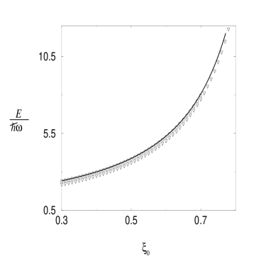
FIG. 2a.: The energy spectrum for $n_{x}=0$: the full line is the exact spectrum, triangles are the zeros of the second branch and circles - the zeros of the third branch.

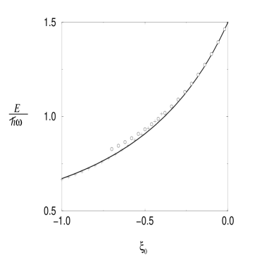
FIG. 2b.: The energy spectrum for $n_{x}=0$: circles are the zeros of the fourth branch, otherwise notations like in Fig. 2a.

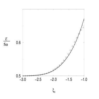
FIG. 2c.: The energy spectrum for $n_{x}=0$: triangles are the zeros of the fifth branch, otherwise notations like in Fig. 2b.

FIG. 3.: The energy spectrum of the disc as function of the magnetic flux. The energy $E$ in the vertical axis is in units of $\frac{2\hbar^{2}}{mR^{2}}$.

FIG. 4.: The energy spectrum of the disc as function of the angular momentum ($N_{\Phi}=20$): circles are the zeros of the third branch, pluses - the zeros of the fourth branch and triangles are the zeros of the fifth branch.

REFERENCES

- [1] Present address:Institut de Recherche sur les Systèmes Atomiques et Moléculaires Complexes (IRSAMC), Université Paul Sabatier, 118 route de Narbonne, Toulouse Cedex 04, France
- [2] Levy L P, Reich D H, Pfeiffer L and West K 1993 Physica B 189 204
- [3] Nakamura K, Thomas H 1988 Phys. Rev. Lett. 61 247
- [4] Ullmo D, Richter K, Jalabert R A 1995 Phys. Rev. Lett. 74 383; for a review see Richter K, Ullmo D, Jalabert R A 1996 Phys. Reports 276 1
- [5] Laughlin R B 1981, Phys Rev B 23 5632; MacDonald A H and Středa P 1984 Phys. Rev. B 29 1616; Halperin B I 1982 Phys. Rev. B 25 2185
- [6] Brillouin M L 1926 J. de Physique (Ser. 6) 7 355; Keller J B 1958 Ann. Phys. (N.Y.) 4 180
- [7] Isihara A and Ebina K 1988 J. Phys. C (Solid State) 21 L1079
- [8] Berry M V, Mount K E 1972 Rep. Prog. Phys. 35 315
- [9] Miller S C and Good R H 1953 Phys. Rev. 91 174
- [10] Bender C M and Orszag S A 1978 Advanced Mathematical Methods for Scientists and Engineers (McGraw Hill: New York)
- [11] Keller J B and Rubinow S I 1960 Ann. Phys. N.Y. 9 24
- [12] Abramowitz M and Stegun I A (eds) 1972 Handbook of mathematical functions (National Bureau of Standards: Washington, D. C.)
- [13] Langer R E 1937 Phys. Rev. 51 669
- [14] Kramers H A 1926 Z. Phys. 39 828
- [15] Gurevich E and Shapiro B 1997 J. Phys. I France 7 807
- [16] Dingle R B 1952 Proc. Roy. Soc. A 212 47
- [17] Blaschke J, Brack M 1997 Phys. Rev. A 56 182
- [18] Akkermans E, Avron J E, Narevich R and Seiler R 1996 cond-mat/9612063
- [19] Atiyah M F, Patodi V K and Singer I M 1975 Math. Proc. Camb. Phil. Soc. 77 43
- [20] Frahm K M and Shepelyansky D L 1997 Phys. Rev. Lett. 78 1440; Frahm K M 1997 Phys. Rev. B 55 8626
- [21] Primack H, Schanz H, Smilansky U and Ussishkin I 1996 Phys. Rev. Lett. 76 1615; Sieber M, Pavloff N and Schmit C 1997 Phys. Rev. E 55 2279