Bose-Einstein Condensation in a Confined Geometry with and without a Vortex

1 Introduction

Much attention has been focused on many-body dilute Bose systems since the discovery of Bose-Einstein condensation (BEC) in alkali atom gases at ultra-low temperatures around $O(\mu K)\sim O(nK)~{}$.${}^{\hbox{\immediate{\bf{?}},\penalty 1000\hskip 0.91003pt plus 0.70004pt minus 0.70004pt{\bf{?}},\penalty 1000\hskip 0.91003pt plus 0.70004pt minus 0.70004pt{\bf{?}})}}$ The current experiments ${}^{\hbox{\immediate{\bf{?}})}}$ performed on atomic gases such as sodium and rubidium in confined geometries trapped by a magnetic field and/or optical method. Furious experimental and theoretical investigations are now ongoing and rapidly developing. Since these atom gases are dilute Bose systems, allowing us to model these as weakly interacting many-body Bose systems, it is regarded as realization of ideal Bose-Einstein condensation. Although superfluid ⁴He has been considered as the first BEC, the mutual repulsive interaction is rather strong where the condensate fraction only $\sim$10$\%$ of the total. There is little chance to directly apply microscopic theory to it.

The microscopic theoretical work on BEC started with Bogoliubov ,${}^{\hbox{\immediate{\bf{?}})}}$ followed by several important progresses, such as Gross ,${}^{\hbox{\immediate{\bf{?}})}}$ Pitaevskii ,${}^{\hbox{\immediate{\bf{?}})}}$ Iordanskii ,${}^{\hbox{\immediate{\bf{?}})}}$ and Fetter .${}^{\hbox{\immediate{\bf{?}})}}$ They treat an infinite system. These mean-field theories ${}^{\hbox{\immediate{\bf{?}})}}$ are particularly suited for treating an spatially non-uniform system which is the case of the present gaseous BEC systems trapped optically or magnetically in a restricted geometry. Therefore, the current theoretical studies ${}^{\hbox{\immediate{\bf{?}})}}$ mainly focus on examining these mean field theories at various stages of the employed approximation for dilute Bose gases trapped by the usually harmonic potential in order to extract the spatial structures of the condensate and non-condensate and low-lying collective modes. Agreement between these mean field theories and experiments is generally fairly good so far, encouraging us to go along this line.

The purposes of this paper are two-fold: One is to compare various approximate treatments: (1) the Gross-Pitaevskii approximation (GP), which considers only the condensate, (2) the Bogoliubov approximation (BA), which takes into account the non-condensate too, but not self-consistent, (3) the Popov approximation (PA), which neglects the anomalous correlation and (4) the Hartree-Fock Bogoliubov approximation (HFB). (3) and (4) take into account the condensate and non-condensate self-consistently. We obtain a complete self-consistent solution numerically for these four cases on an equal footing. This has not been done before. This is particularly true for HFB whose detailed study has not been performed. These various approximate theories reveal both merits and demerits. None is complete and satisfactory. Nevertheless we may gain some insights to general properties of trapped BEC systems.

The second purpose, which is the main purpose, is to know various properties of the quantized vortex structure in rotating BEC systems since microscopic treatment of the vortex has been lacking so far except for a few attempts based on GP ${}^{\hbox{\immediate{\bf{?}})}}$ for present BEC systems. We are particularly interested in understanding (A) the spatial profiles of the condensate, non-condensate and anomalous correlation, (B) the dispersion relation of the excitation spectrum of the system, and (C) the low-lying excitations localized around a vortex core in detail, which is known as the Kelvin mode .${}^{\hbox{\immediate{\bf{?}})}}$ These features should be compared with those in vortices in a superconductor where extensive studies have been compiled .${}^{\hbox{\immediate{\bf{?}})}}$ This is particularly true for the localized excitations near a vortex core studied by Caroli et al. .${}^{\hbox{\immediate{\bf{?}})}}$ The HFB theory just corresponds to the so-called Bogoliubov de Gennes theory (BdG), which is widely used to treat various spatially non-uniform superconductors having interface or vortex. In particular, Gygi and Schlüter ${}^{\hbox{\immediate{\bf{?}})}}$ have done a detailed investigation on an isolated vortex, providing a fairly complete and clear picture of microscopic structures for quantized vortex in a s-wave superconductor.

We have been motivated by their impressive work and considered that a similar work should be done in a BEC system because vortex in BEC might be eventually observed and the vortex core structure and associated low-lying excitations may be probed experimentally. The characteristic core radius is estimated as the coherence length $\sim 0.1\mu$m which contrasted with a few $\AA$ in superfluid ⁴He. Thus there is a good chance to investigate the detailed core structure of the present BEC systems. In a superconductor scanning electron microscopy by Hess et al. ${}^{\hbox{\immediate{\bf{?}})}}$ directly gives vivid spatially resolved images of the low-lying excitations near a vortex core.

It turns out that although the full self-consistent HFB solution obtained here shows some fundamental unsatisfactory caveats of the gapfull excitation which are not in BdG, we believe that the present study is of still some use, because the overall features of the resulting vortex picture are expected to be independent of the approximations. These physical quantities obtained here may be directly observable once the experiment succeeds in creating a vortex.

In his series of papers Fetter ${}^{\hbox{\immediate{?})}}$ investigates the vortex structure in an imperfect Bose gas within the Bogoliubov approximation, giving an approximate analytic treatment for an infinite system: Although he succeeded in deriving asymptotic behaviors of several physical quantities, such as the non-condensate fraction at the core using the approximately obtained eigenfunctions on the basis of the work by Pitaevskii ${}^{\hbox{\immediate{?})}}$ and Iordanskii ${}^{\hbox{\immediate{?})}}$ who solve the Bogoliubov equation for the particular angular momentum states: $q_{\theta}=-1$ and $q_{\theta}=1$ respectively ($q_{\theta}$ is defined shortly). Hence the problem with the rotating BEC in the Bogoliubov theory is not solved completely even for an infinite system. Thus no one has analyzed it for a finite trapped system.

In next Section a brief description of the Hartree-Fock Bogoliubov theory (HFB) is given. In this process various approximate treatments mentioned above are introduced. We explain how to solve a set of the HFB equations numerically in a self-consistent manner, following the method devised by Gygi and Schlüter .${}^{\hbox{\immediate{?})}}$ Here we consider a cylindrically symmetric case with a rigid wall and choose parameters appropriate to present BEC systems for ²³Na and ⁸⁷Rb. The results for stationary non-uniform case are presented in §3. The vortex structure is discussed in details within HFB which turns out to be only stable theory among the above theories except for GP when the system rotates around the symmetry axis in §4. The final section is devoted to discussions and summary.

2 Formulation and Numerical Procedure

2.1 Various Approximations

We start with the following Hamiltonian in which Bose particles interact with a two-body potential $V_{\rm int}$:

$$\hat{\rm H} = \int{\rm d}{\bf r}\hat{\Psi}^{\dagger}({\bf r})\left\{-\frac{\hbar^{2}\nabla^{2}}{2m}+V_{\rm ext}({\bf r})-\mu\right\}\hat{\Psi}({\bf r})$$ (1)

$$+\frac{1}{2}\!\!\int\!\!{\rm d}{\bf r}_{1}\!\!\!\int\!\!{\rm d}{\bf r}_{2}\hat{\Psi}^{\dagger}({\bf r}_{1})\hat{\Psi}^{\dagger}({\bf r}_{2})V_{{\rm int}}({\bf r}_{1}-{\bf r}_{2})\hat{\Psi}({\bf r}_{2})\hat{\Psi}({\bf r}_{1})$$

where the chemical potential $\mu$ is introduced to fix the particle number and $V_{{\rm ext}}({\bf r})$ is the confining potential. In order to describe the Bose condensation, we assume that the field operator $\hat{\Psi}$ is decomposed into

$$\hat{\Psi}=\hat{\psi}({\bf r})+\phi({\bf r})$$ (2)

where the ground state average is given by

$$\langle\hat{\Psi}({\bf r})\rangle=\phi({\bf r}).$$ (3)

A c-number $\phi({\bf r})$ corresponds to the condensate wave function and $\hat{\psi}({\bf r})$ is a q-number describing the non-condensate. The two-body interaction $V_{\rm int}({\bf r}_{1}-{\bf r}_{2})$ is assumed to be $g\delta({\bf r}_{1}-{\bf r}_{2})$ with $g$ being a positive (repulsive) constant proportional to the s-wave scattering length $a$, namely $g=4\pi\hbar^{2}a/m$ ($m$ the particle mass). Substituting the above decomposition (2) in (1), we obtain

$$\hat{{\rm H}} = \int{\rm d}{\bf r}\Bigl{[}\phi^{*}({\bf r})h({\bf r})\phi({\bf r})+{1\over 2}g|\phi|^{4}$$ (4)

$$+\hat{\psi}^{\dagger}({\bf r})\left\{h({\bf r})+g|\phi({\bf r})|^{2}\right\}\phi({\bf r})+{\rm h.c.}$$

$$+\hat{\psi}^{\dagger}({\bf r})\left\{h({\bf r})+2g|\phi({\bf r})|^{2}\right\}\hat{\psi}({\bf r})$$

$$+\frac{g}{2}\hat{\psi}^{\dagger}({\bf r})\hat{\psi}^{\dagger}({\bf r})\phi({\bf r})\phi({\bf r})+{\rm h.c.}$$

$$+g\hat{\psi}^{\dagger}({\bf r})\hat{\psi}({\bf r})\hat{\psi}({\bf r})\phi^{*}({\bf r})+{\rm h.c.}$$

$$+\frac{g}{2}\hat{\psi}^{\dagger}({\bf r})\hat{\psi}^{\dagger}({\bf r})\hat{\psi}({\bf r})\hat{\psi}({\bf r})\Bigr{]}$$

with

$$h({\bf r})\equiv-\frac{\hbar^{2}\nabla^{2}}{2m}+V_{\rm ext}({\bf r})-\mu$$ (5)

one-body Hamiltonian. Let us introduce the variational parameters: the non-condensate density $\rho({\bf r})=\langle\hat{\psi}^{\dagger}({\bf r})\hat{\psi}({\bf r})\rangle$ and the anomalous correlation $\Delta({\bf r})=\langle\hat{\psi}({\bf r})\hat{\psi}({\bf r})\rangle$ and approximate as

$$\hat{\psi}^{\dagger}\hat{\psi}\hat{\psi} = 2\hat{\psi}\rho+\hat{\psi}^{\dagger}\Delta$$ (6)

$$\hat{\psi}^{\dagger}\hat{\psi}^{\dagger}\hat{\psi}\hat{\psi} = \hat{\psi}^{\dagger}\hat{\psi}^{\dagger}\Delta+\hat{\psi}\hat{\psi}\Delta^{*}+4\hat{\psi}^{\dagger}\hat{\psi}\rho.$$ (7)

Then, $\hat{\rm H}$ is rewritten as

$$\hat{\rm H} = \int\!{\rm d}{\bf r}\Bigl{[}\Bigl{\{}\phi^{*}({\bf r})h({\bf r})\phi({\bf r})+{1\over 2}g|\phi|^{4}\Bigr{\}}$$ (8)

$$+\hat{\psi}^{\dagger}({\bf r})\bigl{\{}h({\bf r})+g|\phi({\bf r})|^{2}+2g\rho({\bf r})\bigr{\}}\phi({\bf r})+{\rm h.c.}$$

$$+\hat{\psi}^{\dagger}({\bf r})g\Delta({\bf r})\phi^{*}({\bf r})+{\rm h.c.}$$

$$+\hat{\psi}^{\dagger}({\bf r})\left\{h({\bf r})+2g|\phi({\bf r})|^{2}+2g\rho({\bf r})\right\}\hat{\psi}({\bf r})$$

$$+\frac{g}{2}\hat{\psi}^{\dagger}({\bf r})\left\{\Delta({\bf r})+\phi^{2}({\bf r})\right\}\hat{\psi}^{\dagger}({\bf r})+{\rm h.c.}\Bigr{]}.$$

In order to diagonalize this Hamiltonian, the following Bogoliubov transformation is employed, namely, $\hat{\psi}({\bf r})$ is written in terms of the creation and annihilation operators $\eta_{q}$ and $\eta_{q}^{\dagger}$ and the non-condensate wave functions $u_{q}({\bf r})$ and $v_{q}({\bf r})$ as

$$\hat{\psi}({\bf r})=\sum_{{\it q}}\left[u_{q}({\bf r})\eta_{q}-v_{q}^{*}({\bf r})\eta_{q}^{\dagger}\right]$$ (9)

where $q$ denotes the quantum number. This leads to the diagonalized form:

$$\hat{\rm H}={\rm E}_{0}+\sum_{q}E_{q}\eta_{q}^{\dagger}\eta_{q}.$$ (10)

The condition that the first order term in $\hat{\psi}({\bf r})$ vanish yields

$$\{h({\bf r})+g|\phi({\bf r})|^{2}+2g\rho({\bf r})\}\phi({\bf r})+g\Delta({\bf r})\phi^{*}({\bf r})=0.$$ (11)

When $\rho({\bf r})$ and $\Delta({\bf r})$ are made zero, it reduces to the Gross-Pitaevskii (GP) equation:

$$h({\bf r})\phi({\bf r})+g\phi^{*}({\bf r})\phi({\bf r})\phi({\bf r})=0,$$ (12)

which is a non-linear Schrödinger type equation.

The condition that the Hamiltonian be diagonalized gives rise to the following set of eigenvalue equations for $u_{q}({\bf r})$ and $v_{q}({\bf r})$ with the eigenvalue $E_{q}$:

$$\left[h({\bf r})+2g\{\rho({\bf r})+|\phi({\bf r})|^{2}\}\right]u_{q}({\bf r})$$

$$-g\left[\Delta({\bf r})+\phi^{2}({\bf r})\right]v_{q}({\bf r}) = E_{q}u_{q}({\bf r})$$ (13)

$$\left[h({\bf r})+2g\{\rho({\bf r})+|\phi({\bf r})|^{2}\}\right]v_{q}({\bf r})$$

$$-g\left[\Delta^{*}({\bf r})+\phi^{*2}({\bf r})\right]u_{q}({\bf r}) = -E_{q}v_{q}({\bf r}).$$ (14)

The eigenvectors $u_{q}({\bf r})$ and $v_{q}({\bf r})$ must satisfy the normalization condition:

$$\int\left\{u_{p}^{*}({\bf r})u_{q}({\bf r})-v_{p}^{*}({\bf r})v_{q}({\bf r})\right\}{\rm d}{\bf r}=\delta_{p,q}.$$ (15)

The variational parameters $\rho({\bf r})$ and $\Delta({\bf r})$ are determined self-consistently by

$$\rho({\bf r}) = \langle\hat{\psi}^{\dagger}\hat{\psi}\rangle$$

$$= \sum_{\it q}(|u_{q}({\bf r})|^{2}+|v_{q}({\bf r})|^{2})f(E_{q})+\sum_{\it q}|v_{q}({\bf r})|^{2}$$

$$\Delta({\bf r}) = \langle\hat{\psi}\hat{\psi}\rangle$$

$$= -\sum_{{\it q}}2u_{q}({\bf r})v_{q}^{*}({\bf r})f(E_{q})-\sum_{\it q}u_{q}({\bf r})v_{q}^{*}({\bf r})$$

where $f(E)$ is the Bose distribution function. At absolute zero temperature, which we consider from now on, these become

$$\rho({\bf r}) = \sum_{{\it q}}v_{q}^{*}({\bf r})v_{q}({\bf r})$$ (16)

$$\Delta({\bf r}) = -\sum_{{\it q}}u_{q}({\bf r})v_{q}^{*}({\bf r}).$$ (17)

Equations (11), (13), (14), (16) and (17) constitute a complete set of the self-consistent equations for the Hatree-Fock Bogoliubov theory (HFB). If $\rho({\bf r})$ and $\Delta({\bf r})$ are made to zero, we recover the Bogoliubov theory (BA). The Popov approximation (PA) is the case of $\Delta({\bf r})=0$ in HFB. In the followings, we perform these four cases, namely, GP, BA, PA and HFB in the equal footing to comparatively study similarities and differences.

The expectation value of the particle number density is given as

$$\langle\hat{\rm n}({\bf r})\rangle=|\phi({\bf r})|^{2}+\rho({\bf r}),$$ (18)

that is, the total density consists of the condensate part $\phi({\bf r})$ and the non-condensate part $\rho({\bf r})$. The particle current density is calculated,

$${\bf j}({\bf r}) = \frac{\hbar}{2m{\rm i}}\{\phi^{*}({\bf r})\nabla\phi({\bf r})-\phi({\bf r})\nabla\phi^{*}({\bf r})\}$$ (19)

$$+\frac{\hbar}{2m{\rm i}}\langle\hat{\psi}^{\dagger}({\bf r})\cdot\nabla\hat{\psi}({\bf r})-\nabla\hat{\psi}^{\dagger}({\bf r})\cdot\hat{\psi}({\bf r})\rangle.$$

2.2 Numerical Procedure

For later convenience, we introduce the following non-dimensional quantities: In terms of the mass $m$ and the average particle number density $n_{a}$, the various densities and the length are scaled by $n_{a}$ and $\xi_{a}\equiv{\hbar^{2}}/{\sqrt{2mn_{a}g}}$ respectively. $\xi_{a}$ is the coherence length of the condensate given by solving the above GP equation (12). The energy is scaled by $n_{a}g$. We define the quantities: ${\bf r}^{\prime}\equiv\frac{1}{\xi_{a}}{\bf r}$, $\phi^{\prime}({\bf r}^{\prime})\equiv\frac{1}{\sqrt{n_{a}}}\phi({\bf r})$, $\rho^{\prime}({\bf r}^{\prime})\equiv\frac{1}{n_{a}}\rho({\bf r})$, $\Delta^{\prime}({\bf r}^{\prime})\equiv\frac{1}{n_{a}}\Delta({\bf r})$, $u^{\prime}({\bf r}^{\prime})\equiv\frac{1}{\sqrt{n_{a}}}u({\bf r})$, $v^{\prime}({\bf r}^{\prime})\equiv\frac{1}{\sqrt{n_{a}}}v({\bf r})$, $E^{\prime}_{q}\equiv\frac{1}{n_{a}g}E_{q}$. The system is now characterized by $n_{a}\xi_{a}^{3}$ and the system volume normalized by $\xi_{a}$. From now on, we suppress primes $\prime$ in these newly defined quantities. Note that by increasing the average density $n_{a}$ the effective interaction gets stronger, namely the tuning of the interaction by controlling an external parameter $n_{a}$ is an interesting and important aspect of the BEC system.

We now consider a cylindrically symmetric system which is characterized by the radius $R$ and the height $L$. We impose the boundary conditions that in terms of the cylindrical coordinate: ${\bf r}=(r,\theta,z)$ the all wave functions vanish at the wall $r=R$ and the periodic boundary condition along the $z$-axis. When a vortex line passes through the center of the cylinder the condensate wave function $\phi({\bf r})$ is expresses as

$$\phi(r,\theta,z)=\phi(r)e^{{\rm i}w\theta}$$ (20)

where $\phi(r)$ is a real function and $w$ is the winding number. $w=0$ corresponds to non-vortex case and $w=1$ to the vortex case. The $w\geq 2$ case is not considered here because this state is energetically unstable. The non-condensate density $\rho$ is a real function, depending only on $r$ that is, $\rho(r,\theta,z)=\rho(r)$. It is seen from eq. (11) that the anomalous correlation $\Delta$ has the phase with 2$\theta$, thus $\Delta(r,\theta,z)=\Delta(r)e^{2{\rm i}w\theta}$. It is also seen from eqs. (13) and (14) that the phases of $u_{q}({\bf r})$ and $v_{q}({\bf r})$ are written as

$$u_{\bf q}({\bf r}) = u_{\bf q}(r)e^{{\rm i}q_{z}z}e^{{\rm i}(q_{\theta}+w)\theta}$$ (21)

$$v_{\bf q}({\bf r}) = v_{\bf q}(r)e^{{\rm i}q_{z}z}e^{{\rm i}(q_{\theta}-w)\theta}.$$ (22)

The set of the quantum numbers ${\bf q}$ in (9) is described by $(q_{r},q_{\theta},q_{z})$ where $q_{r}=1,2,3,\cdots$, $q_{\theta}=0,\pm 1,\pm 2,\cdots$, $q_{z}=0,\pm 2\pi/L,\pm 4\pi/L,\cdots$.

The functions $u_{q}(r)$ and $v_{q}(r)$ are expanded in terms of

$$\varphi_{\mu}^{(i)}(r)\equiv\frac{\sqrt{2}}{J_{|\mu|+1}\left(\alpha_{\mu}^{(i)}\right)}J_{|\mu|}\left(\alpha_{\mu}^{(i)}\frac{r}{R}\right)$$ (23)

as

$$u_{q}(r) = \sum_{i}c_{q}^{(i)}\varphi_{q_{\theta}+w}^{(i)}(r)$$ (24)

$$v_{q}(r) = \sum_{i}d_{q}^{(i)}\varphi_{q_{\theta}-w}^{(i)}(r)$$ (25)

where $J_{\mu}(r)$ is the Bessel function of $\mu$-th order and $\alpha_{\mu}^{(i)}$ denotes $i$-th zero of $J_{\mu}$.

Then, eq. (11) becomes

$$-\left\{\frac{{\rm d}^{2}\phi}{{\rm d}r^{2}}+\frac{1}{r}\frac{{\rm d}\phi}{{\rm d}r}-\frac{w^{2}}{r^{2}}\phi\right\}$$

$$+\left\{V_{\rm ext}-\mu+\phi^{2}+2\rho+\Delta\right\}\phi = 0.$$ (26)

The eigenvalue problem of eqs. (13) and (14) reduces to diagonalizing the matrix:

$$\left(\!\!\!\!\begin{array}[]{cc}A_{i,j}(q_{\theta}+w,q_{z})&-B_{i,j}(q_{\theta},w)\\ &\\ B_{i,j}^{\rm T}(q_{\theta},w)&-A_{i,j}(q_{\theta}-w,q_{z})\end{array}\!\!\!\!\right)\!\!\!\left(\!\!\!\!\begin{array}[]{c}c_{\bf q}^{(1)}\\ c_{\bf q}^{(2)}\\ \vdots\\ d_{\bf q}^{(1)}\\ d_{\bf q}^{(2)}\\ \vdots\end{array}\!\!\!\!\right)\!=\!E_{\bf q}\!\!\left(\!\!\!\!\begin{array}[]{c}c_{\bf q}^{(1)}\\ c_{\bf q}^{(2)}\\ \vdots\\ d_{\bf q}^{(1)}\\ d_{\bf q}^{(2)}\\ \vdots\end{array}\!\!\!\!\right)$$ (27)

$$A_{i,j}(\mu,q_{z}) = \left\{\left(\frac{\alpha_{\mu}^{(j)}}{R}\right)^{2}+q_{z}^{2}-\mu\right\}\delta_{i,j}$$ (28)

$$+\int_{0}^{R}\!\!\left(V_{\rm ext}+2(\phi^{2}+\rho)\right)\varphi_{\mu}^{(i)}\varphi_{\mu}^{(j)}r\,{\rm d}r$$

$$B_{i,j}(q_{\theta},w) = \int_{0}^{R}\left(\Delta+\phi^{2}\right)\varphi_{q_{\theta}+w}^{(i)}\varphi_{q_{\theta}-w}^{(j)}r\,{\rm d}r$$ (29)

where ${\bf q}=(q_{r},q_{\theta},q_{z})$. The normalization condition (15) of the eigenvectors is rewritten in terms of $c^{(i)}_{\bf q}$ and $d^{(i)}_{\bf q}$ as

$$n_{a}\xi_{a}^{3}\sum_{i}\left\{c_{\bf p}^{(i)}c_{\bf q}^{(i)}-d_{\bf p}^{(i)}d_{\bf q}^{(i)}\right\}=\frac{1}{2\pi L}\delta_{{\bf p},{\bf q}}.$$ (30)

From eqs. (16) and (17) $\rho(r)$ and $\Delta(r)$ are determined by

$$\rho(r) = \sum_{{\bf q},i}(d_{\bf q}^{(i)}\varphi_{q_{\theta}-w}^{(i)})^{2}$$ (31)

$$\Delta(r) = -\sum_{{\bf q},i,j}c_{\bf q}^{(i)}d_{\bf q}^{(j)}\varphi_{q_{\theta}+w}^{(i)}\varphi_{q_{\theta}-w}^{(j)}.$$ (32)

The iterative calculations of eqs. (26), (27), (31), and (32) yield a convergent self-consistent solution. It is not self-evident a priori that eq. (27) gives real eigenvalues because the Hamiltonian matrix in eq. (27) is not symmetric. Note that since $q_{\theta}$ is the angular momentum and $q_{z}=2\pi n/L$ ($n$ integer) is the wave number along the $z$-axis, both being good quantum numbers, the eigenvalue equation (27) is decomposed into each $q_{\theta}$ and $q_{z}$. Each block-diagonal eigenvalue equation gives rise to the quantum number $q_{r}$ along the radial direction $r$.

2.3 Calculated System

As mentioned, our system is characterized by the two parameters: the reduced density $n_{a}\xi_{a}^{3}$ and the system size $R$ and $L$ (in unites of $\xi_{a}$). The interaction strength characterized by the scattering length $a$ is absorbed in the reduced density. We set $n_{a}\xi_{a}^{3}=1.0$, $R=15$, and $L=30$ throughout this paper. We are treating 2.12$\times 10^{4}$ atoms. Since the scattering length of Rb is known as $a$=5.8nm, the energy scale $n_{a}g\sim 10^{-30}$J. These numbers are compared with the experiment by Anderson et al. .${}^{\hbox{\immediate{?})}}$ The radius of the condensate $\sim 10\mu$m, the trapping potential energy $\sim 10^{-28}$J and the total number of atoms $\sim$10³. Similar set of the numbers are obtained for the Na experiment .${}^{\hbox{\immediate{?})}}$

We have employed the two methods for numerical calculation: the momentum cutoff method and the energy cutoff method to check our numerical accuracy. In the former, the computation is limited to certain finite quantum numbers for $q_{r}$, $q_{\theta}$, and $q_{z}$. We have examined several cases where -50$\leq$$q_{\theta}$, $q_{z}$$\leq$+50 and -75$\leq$$q_{\theta}$, $q_{z}$$\leq$+75, keeping the maximum number of $q_{r}\sim 50$ fixed. In view of the tendency of the obtained solutions, the last case is satisfactory, thus the total number of the treated eigenfunctions $\sim 500000$ because the size dependence on $q_{\theta}$ and $q_{z}$ almost ceases stopping. In the energy cutoff method where the calculation terminates when the obtained eigenvalues exceeds a certain value, typically, 100, and 200 in the units of $n_{a}g$. The last case which treats $\sim 500000$ eigenfunctions seems best in view of the expected behavior of the solutions. Note that the anomalous correlation $\Delta$ is most dependent on this cutoff condition while $\rho$ is relatively insensitive. Comparing the two methods, the energy cutoff method is better than the momentum cutoff method, thus we show the results employed this method below.

3 Stationary non-uniform case

In order to examine the accuracy of the numerical computations and to know the properties of BEC in the stationary state, we first consider non-vortex Bose system confined in a cylindrical vessel. The corresponding infinite system is analyzed by, for example, Fetter ${}^{\hbox{\immediate{?})}}$ within the Bogoliubov approximation (BA).

The condensate $\phi({\bf r})$ is shown in Fig. 1 where GP and BA give the same result for this quantity, since BA neglects the non-condensate and the anomalous correlation. It is seen that PA and HFB give nearly same results as that in GP (or BA) because the absolute values of $\rho$ and $\Delta$ are very small for our parameter selected. Thus this is not the general conclusion. The condensate fraction could decrease as $g$ or $n_{a}$ increases. The overall behaviors of these results are quite understandable; The condensate changes only near the wall, whose characteristic length is the coherent length $\xi_{a}$ introduced before. The expected flatness in the bulk region around the center indicates the reliability of our numerical calculations.

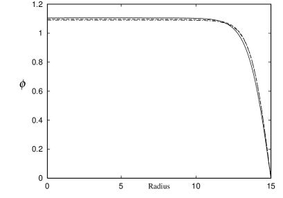
Fig.  1: Spatial variation of the condensate $\phi(r)$ as a function of $r$ for HFB (bold line), PA (dot dashed line), and GP and BA (dashed line).

The spatial profiles of the non-condensate $\rho({\bf r})$ for various approximations are displayed in Fig. 2. $\rho({\bf r})$ in BA is calculated by using eq. (16) where $u(r)$ and $v(r)$ are a solution in BA and is shown for reference. While BA and PA give a similar variation, the magnitude of $\rho({\bf r})$ in HFB is almost halved. This difference may be related to $\Delta$ in HFB. It is noted that $\rho(0)\sim 0.014$ in BA and PA compared with the analytic expression at $T$=0

$$\rho={1\over 6\pi^{2}{\sqrt{2}}\xi^{3}n_{0}}\sim 0.012{1\over\xi^{3}n_{0}}$$ (33)

by Fetter ${}^{\hbox{\immediate{?})}}$ for an infinite system ($n_{0}$ the average number density and $\xi=\hbar/\sqrt{2mn_{0}g}$) whose number $\rho=0.012$ in the present case ($\xi^{3}n_{0}$=1.0). The small difference comes from the system size (finite vs infinite). In fact in our calculations the limiting value $\rho=0.012$ are slowly recovered as the system size increases. The major spatial variation only occurs at the wall whose length is an order of $\xi_{a}$. Note from Fig. 2 that $\rho$ vanishes quadratically instead of linearly in $\phi(r)$.

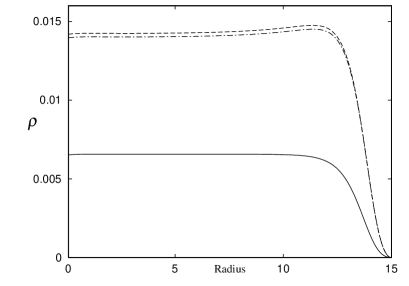
Fig.  2: Spatial variation of the non-condensate $\rho(r)$ as a function of $r$ for HFB (bold line), PA (dot dashed line), and BA (dashed line).

The anomalous correlation $\Delta(r)$ is shown in Fig. 3 where BA and HFB are compared. The amplitude $\Delta(r)$ in HFB at the center are rather large and negative, which affects mainly on $\rho(r)$, namely, the large difference of $\rho(r)$ between BA and PA, and HFB comes from the absence or presence of $\Delta(r)$. It is noted also that $|\Delta(r)|$ in the bulk region sensitively depends on the calculated system size which is contrasted with other quantities such as $\phi(r)$ or $\rho(r)$. It should be noticed also that as mentioned above the expected flat behavior far from the wall is reproduced only when the enough number of the eigenfunctions are taken account in the numerical computation, otherwise this particular quantity $\Delta(r)$ often fails to exhibit the expected flat behavior.

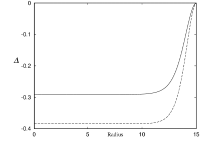
Fig.  3: Spatial variation of the anomalous correlation $\Delta(r)$ as a function of $r$ for HFB (bold line) and BA (dashed line).

In Figs. 4(a), (b), and (c) where the eigenvalues $E({\bf q})$ are plotted as functions of the quantum numbers of $q_{\theta}$ and $q_{z}$, the excitation spectra are shown for BA and HFB. The spectrum in PA which is not shown here is almost identical to that in BA. Indeed, the excitation spectrum in PA and BA is gapless while HFB is gapful as expected .${}^{\hbox{\immediate{\bf{?}})}}$ In BA the so-called Bogoliubov spectrum ${}^{\hbox{\immediate{?})}}$ $E^{B}({\bf k})$ is known to be given by

$$E^{B}({\bf k})=\sqrt{\epsilon^{2}_{k}+2\epsilon_{k}n_{0}g}$$ (34)

where $\epsilon_{k}={\hbar^{2}{\bf k}^{2}\over 2m}$. In the long wavelength limit it reduces to

$$E^{B}({\bf k})\sim\hbar ck\ \ \ \ \ {\rm for}\ \ \ \ k\rightarrow 0$$ (35)

where $c=\sqrt{{n_{0}g\over m}}$. The low-lying excitations are known to be exhausted by phonons ($c$ is the sound velocity) .${}^{\hbox{\immediate{\bf{?}})}}$ In the short wavelength limit it becomes

$$E^{B}({\bf k})\sim{\hbar^{2}{\bf k}^{2}\over 2m}\ \ {\rm for}\ \ k\rightarrow\infty.$$ (36)

where the excitations are individual one-particle excitation. These expected behaviors in BA are well reproduced by the present calculations; As seen from Figs. 4(a) and 4(b), the dispersion relations in BA and PA are linear in $q\rightarrow 0$ and quadratic in $q\rightarrow\infty$ where $k_{z}={2\pi\over L}q_{z}$. In fact, the theoretical lines of eqs. (35) and (36) drawn in Figs. 4(a) and 4(b) show good fits to the numerical results without any fitting parameter, proving the reliability of our calculations. On the other hand, as seen from Fig. 4(c) HFB is a gapful theory. This dispersion relation is quadratic in both $q_{\theta}$ and $q_{z}$. The magnitude of this gap is an order of $n_{a}g$.

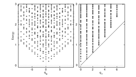
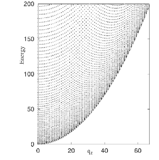
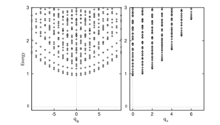
Fig.  4: Excitation spectra as functions of $q_{\theta}$ (left hand side) and $q_{z}$ (right hand side) in BA for the small wave numbers (a) and the overall wave numbers at $q_{\theta}=0$ (b). The analytical expression eq. (35) of the Bogoliubov spectrum in the long-wave length limit (straight line) is drawn in the right hand figure of 4(a), and eq. (36) in the short wave length limit (lower edge parabola) drawn in (b), showing that they agree in those limits. (c) Excitation spectra as functions of $q_{\theta}$ (left hand side) and $q_{z}$ (right hand side) in HFB. Note that it has a gap whose magnitude is about 0.9.

In Fig. 5 we display the local density of states:

$$N(E,r)=\sum_{\bf q}\{|u_{\bf q}(r)|^{2}+|v_{\bf q}(r)|^{2}\}\delta(E_{\bf q}-E)$$ (37)

a combination of the quasi-particle eigenfunctions with the lowest energies in BA (the results for the other approximations are quite similar). It is seen from this that although the weight spreads out to the entire regions, the major one concentrates near the wall boundary.

Fig.  5: Local density of states $N(E,r)$ in the lower energy region for BA. It is noted that the density of states accumulated at the center $r=0$ and the wall $r=15$.

4 Rotating vortex case

Having established the reliability of our numerical method, we now discuss the results of the isolated singly quantized vortex case whose quantization unit is ${h\over m}$. It is expected that a rotating BEC system whose frequency exceeds a certain critical value $\omega_{c}\sim{\hbar\over mR^{3}}\ln{R\over\xi}$ estimated as $\sim 50$rad/s for ⁸⁷Rb ${}^{\hbox{\immediate{\bf{?}})}}$ sustains a quantized vortex line threading along the cylindrically symmetric $z$-axis.

It quickly becomes clear after several numerical trials that the BA and PA do not fulfill a fundamental requirement, that is, the quasi-particle eigenvalues $E({\bf q})$ in eqs. (13) and (14) or eq. (27) for BA ($\rho=0$ and $\Delta=0$) and also for PA ($\Delta=0$) must be positive because the condensate situates at zero energy. The negative eigenvalue means an instability of the vortex state. Thus these approximations cannot be a consistent theory for describing the vortex state. As seen from Table 1 where the quasi-particle eigenvalues $E({\bf q})$ from the lowest energies are listed for BA and HFB, the lowest eigenvalue with $q_{\theta}=-1$, $q_{z}=0$ and $q_{r}=1$ in BA is negative. We have checked the negative eigenvalue in BA by changing several conditions: The system size ($R$, $L$), the interaction strength, and the Hamiltonian matrix size. The negative eigenvalue belonging to the lowest energy in BA always exists and is not an artifact of our numerical computations. As for PA, the lowest eigenvalue with the same quantum number mentioned above becomes also a negative number, which always appears at every steps of the iteration processes for self-consistency. We never complete a self-consistency and cannot obtain a self-consistent solution. We conclude that PA cannot sustain a stable vortex solution. Thus, we are left with the non self-consistent GP and the full self-consistent HFB which are discussed in full details in the following.

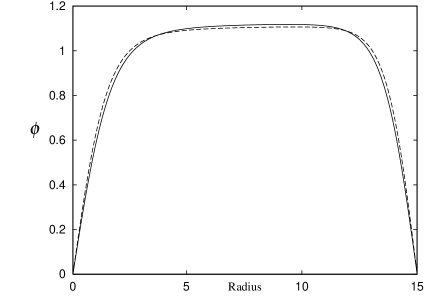
Fig.  6: Spatial variation of the condensate $\phi(r)$ as a function of $r$ for HFB (bold line) and GP (dashed line). It is seen that at the vortex core $r=0$ it vanishes linearly, recovering its bulk value within the characteristic length $\xi_{a}$.

The spatial variations of the condensate $\phi(r)$ in HFB and GP are shown in Fig. 6. It is seen from this that both are almost identical, but the condensate is pushed out in HFB by the presence of the non-condensate, resulting in a slightly larger core radius. This could be further amplified when the interaction $g$ becomes stronger or the atomic density $n_{a}$ becomes high since the non-condensate fraction increases. It is also noticed that understandably $\phi(r)$ is almost symmetric at the middle $r=7.5$ because the characteristic length scale is $\xi_{a}$ in this system, which governs the spatial variation at the core and wall. At the vortex core $\phi(0)=0$ and linearly rises to recover its bulk value shown in Fig. 1. It will be interesting to check if there is a similar Kramer-Pesch effect ${}^{\hbox{\immediate{\bf{?}})}}$ seen in superconductors where the core radius shrinks as temperature decreases. If indeed exists, the core radius increases further as temperature rises. This temperature effect belongs to a future problem. This should be checked experimentally in the present BEC systems because the expected core radius is far larger than that in superfluid ⁴He.

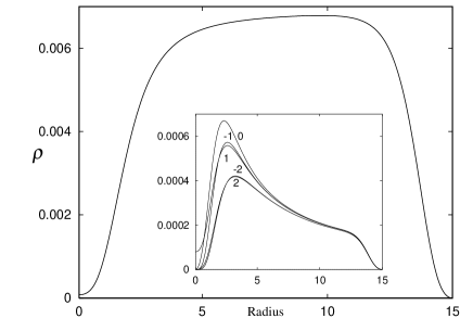
Fig.  7: Spatial variation of the non-condensate $\rho(r)$ as a function of $r$ for HFB. It is seen that $\rho(0)$ is non-vanishing, coming from non-vanishing contribution with $q_{\theta}=0$. The inset shows the contributions from various components characterized by the quantum numbers: $q_{\theta}=0$, $\pm 1$, and $\pm 2$. Note the different scales of the vertical axes.

The non-condensate $\rho(r)$ is displayed in Fig. 7. According to Fetter ,${}^{\hbox{\immediate{?})}}$ a universal relation $\rho(0)/\rho(\infty)\sim$1.4 at $T=0$ is derived for BA, independent of the interaction strength $g$, that is, the amplitude of $\rho(0)$ at the core must exceed that in the outside region. This prediction is not supported by the present calculation in HFB. On the contrary, our result does show a suppression of $\rho(r)$ around the core region whose characteristic length $\sim\xi_{a}$. We do not consider the origin of this discrepancy further because BA is not a stable theory for describing the vortex as mentioned before. In the HFB result, which is a stable solution, $\rho(r)$ recovers the bulk value$\sim$0.006 (see Fig. 2) far from the core where $\rho(0)$ reduces to almost zero. The characteristic recovery length is evidently longer than that in the condensate as seen from Fig. 6. This is partly because the behavior in $\rho(r)$ near the core is quadratic in $r$ while that in $\phi(r)$ is linear. The main contribution to the non-vanishing $\rho(0)$ comes from the component with $q_{\theta}=1$ as seen from the inset of Fig. 7 where other dominant components near the vortex core are also depicted. This also explains the quadratic behavior in $r$ at the core mathematically.

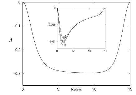
Fig.  8: Spatial variation of the amomalous correlation $\Delta(r)$ as a function of $r$ for HFB. The inset shows the contributions from various components characterized by the quantum numbers: $q_{\theta}=0$, $\pm 1$, and $\pm 2$. Note the different scales of the vertial axes.

The anomalous correlation $\Delta(r)$ is shown in Fig. 8 for HFB, which is no prior prediction and evaluated here for the first time. The sign is negative same as in the non-vortex case of previous section and $\Delta(r)$ vanishes quadratically at the core and also at the wall, recovering its value ($\sim-0.3$) in the bulk (see Fig. 3 for comparison). As shown as the inset where the contributions with the smaller $q_{\theta}$, even near the vortex core there are no distinctive and/or dominant contributions for $\Delta(r)$. As mentioned in §3 this quantity strongly depends on the energy cutoff chosen. If the cutoff energy increases, $|\Delta(r)|$ grows. This feature is absent in the other quantities discussed here.

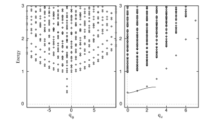
Fig.  9: Excitation spectra as functions of $q_{\theta}$ (left hand side) and $q_{z}$ (right hand side) in HFB. The distinctive modes at $q_{\theta}=-1$ corresponds to the Kelvin wave whose dispersion relation eq. (38) obtained by Pitaevskii ${}^{\hbox{\immediate{?})}}$ in the long wave length is drawn in the right hand side by adjusting the vertical axis for comparison. The bulk of the continuum excitation spectra coincides with those in Fig. 4(c).

In Fig. 9 we exhibit the excitation spectra as functions of $q_{\theta}$ and $q_{z}$ where the distinctive excitations at $q_{\theta}=-1$ are seen, which are isolated from the rest of the continuum seen before (Fig. 4(c)). This particular isolated excitation is known as the Kelvin wave which is present in a vortex of classical liquid and corresponds to a helical mode of the vortex line .${}^{\hbox{\immediate{?})}}$ According to Pitaevkii ${}^{\hbox{\immediate{?})}}$ who found it in BA, at the long wave length limit the dispersion relation is given by

$$E({q_{\theta}=-1},k_{z})={\hbar^{2}k^{2}_{z}\over 2m}\ln{1\over k_{z}\xi_{a}}\ \ \ (k_{z}\xi_{a}\ll 1).$$ (38)

Since this expression is valid only for an infinite system, it is hard to judge whether or not our numerical result for a finite system agrees with this. Apparently, while the eq. (38) is gapless, the present result has a gap. Apart from the gap, our result for the dispersion relation does not contradict this behavior (see the line of eq. (38) drawn Fig.9). The bulk of the gapful continuum in Fig. 9 is just the same as in Fig. 4(c) as expected.

The local density of states given by eq. (37) with the lower energy side are shown in Fig. 10 where the states distinctively localized near the core correspond to the angular momentum $q_{\theta}=-1$. The detailed analyses of eqs. (13) and (14) for $q_{\theta}=-1$ and $q_{\theta}=1$ in BA are performed by Pitaevskii ${}^{\hbox{\immediate{?})}}$ and Iordanskii ${}^{\hbox{\immediate{?})}}$ respectively: $u_{q_{\theta},q_{z}}(r)\sim r^{|q_{\theta}+1|}(1+O(r^{2}))$ and $v_{q_{\theta},q_{z}}(r)\sim r^{|q_{\theta}-1|}(1+O(r^{2}))$ which are easily derived by analyzing eqs. (13) and (14) for BA. Note that only $u_{q_{\theta=-1},q_{z}}(0)$ and $v_{q_{\theta=1},q_{z}}(0)$ are non-vanishing at the core. These properties are also true for the full self-consistent HFB. The local density of states in superconductors is directly observed by scanning tunneling microscope ${}^{\hbox{\immediate{?})}}$ and analyzed theoretically within the similar theoretical framework ${}^{\hbox{\immediate{?})}}$ quite successfully. Since as mentioned before, the core radius in BEC systems is relatively large, there is good chance to directly observe the local excitation spectrum possibly by an optical method once the vortex can be created.

Fig.  10: Local density of states $N(E_{q},r)$ in the lower energy region for HFB. It is noted that the density of states accumulates at the center $r=0$ and the wall $r=15$. The distinctive peak structures come from those with the quantum number $q_{\theta}=-1$, indicating that these modes localize at the vortex core.

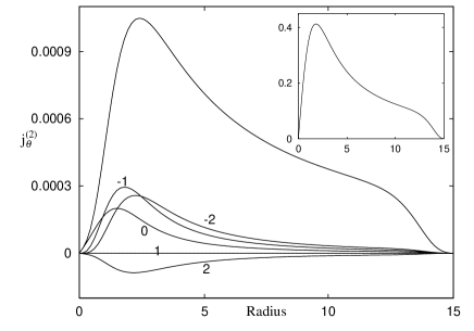
Fig.  11: Current distribution $j^{(2)}_{\theta}(r)$ which comes from the non-condensate where the contributions from the components with $q_{\theta}=-0$,$\pm 1$, and $\pm 2$ are shown. The inset shows the total current $j_{\theta}(r)$. Note that the dominant contribution comes from the condensate. The current is normalized by ${\hbar\over m}\cdot{n_{a}\over\xi_{a}}$.

Finally the circulating current density $j_{\theta}(r)$ for the $\theta$-component which is expressed as

$$j_{\theta}(r) = j^{(1)}_{\theta}(r)+j^{(2)}_{\theta}(r)$$ (39)

$$j^{(1)}_{\theta}(r) = {\hbar\over m}{n_{a}\over\xi_{a}}\cdot{\phi^{2}(r)\over r}$$ (40)

$$j^{(2)}_{\theta}(r) = -{1\over 2{\rm i}r}\cdot{\hbar\over m}{n_{a}\over\xi_{a}}$$ (41)

$$\sum_{\bf q}\left\{v^{\ast}_{\bf q}(r){\partial v_{\bf q}(r)\over\partial\theta}-v_{\bf q}(r){\partial v^{\ast}_{\bf q}(r)\over\partial\theta}\right\}$$

where the total current consists of the condensate component $j^{(1)}_{\theta}(r)$ and the non-condensate $j^{(2)}_{\theta}(r)$. The non-condensate contribution $j^{(2)}_{\theta}(r)$ normalized by ${\hbar\over m}\cdot{n_{a}\over\xi_{a}}$ is depicted for HFB in Fig. 11 where each with $q_{\theta}=0,\pm 1,\pm 2$ is shown separately, and those with smaller $|q_{\theta}|$ dominate near the core. As is seen from Fig. 11 $j^{(2)}_{\theta}(r)$ in the immediate vicinity of the core is governed by the $q_{\theta}=0$ component. The negative (positive) $q_{\theta}$’s give rise to the positive (negative) contribution to $j_{\theta}(r)$. The inset shows the total current density $j_{\theta}(r)$ where $j_{\theta}(r)\sim r$ for small $r$ and $j_{\theta}(r)\sim{1\over r}$ for larger $r$. The relative weights of $j^{(1)}_{\theta}(r)$ and $j^{(2)}_{\theta}(r)$ depends on the interaction strength and the average density $n_{a}$.

5 Conclusion and Discussions

We have investigated various approximate mean-field type theories (Gross-Pitaevskii, Bogoliubov theory, Popov theory and Hartree-Fock Bogoliubov theory) within the framework of the Bogoliubov approximation for a dilute Bose gas, on which renewed interest is focused recently by the discovery of Bose-Einstein condensation in alkali atom gases. The above four type theories are numerically solved for parameters appropriate to ongoing experiments on ²³Na and ⁸⁷Rb atoms and analyzed on an equal footing for the first time. We extract several properties of experimental interest in BEC systems, namely, the spatial structures of the condensate, non-condensate and anomalous correlation both in stationary non-uniform case and the vortex case under rotation. A numerical procedure for solving these mean-field equations are presented and critically assessed for future use.

In the case of the stationary non-uniform Bose gas confined in a cylindrically symmetric vessel the above four theories yield almost identical results for the spatial profile of the condensate. The non self-consistent BA and self-consistent PA and HFB give similar profiles for the non-condensate, but in the last the magnitude are halved.

In the vortex case these mean-field theories are numerically examined. It is found that GP and PA do not fulfill the fundamental requirement, showing an instability of the theories, and thus are inadequate for describing a vortex. The full self-consistent solution for HFB is obtained and analyzed in detail. The spatial structures of the vortex core for Bose systems; the condensate, non-condensate and anomalous correlation are explicitly derived for the first time. Some characteristics of the local density of states and circulating current are pointed out in the hope to be observed in BEC systems in alkali atom gases.

$q_{\theta}$	$q_{z}$	$q_{r}$	Bogoliubov	$q_{\theta}$	$q_{z}$	$q_{r}$	HFB
-1	0	1	-0.01034608886000	-1	0	1	0.35866592764172
0	0	1	0.00222477348689	-1	1	1	0.40521222215704
-1	1	1	0.08359597874556	-1	2	1	0.54360716036381
-1	0	2	0.20124587759088	-1	3	1	0.77139318149905
1	0	1	0.20342514914009	-1	0	2	0.97584202447130
-1	2	1	0.26341740112590	0	0	1	0.98055487186421
-2	0	1	0.28575943668855	-2	0	1	0.98631908786634
0	1	1	0.31282158360176	1	0	1	1.00123548991620
2	0	1	0.35670360464514	-3	0	1	1.01170602030422
-1	1	2	0.35731592142005	-1	1	2	1.02820298664511
1	1	1	0.38616772030053	0	1	1	1.03306239243685
-3	0	1	0.39673767766612	2	0	1	1.03656925663829

Table  I: The lowest energies for the Bogoliubov approximation and the Hartree-Fock Bogoliubov theory (HFB).

References

- [1] M. H. Anderson, J. R. Ensher, M. R. Mathews, C. E. Wieman, and E.A. Cornell: Science, 269 (1995) 198.
- [2] C. C. Bradley, C. A. Sackett, J. J. Tollett, and R. G. Hulet: Phys. Rev. Lett. 75 (1995) 1687.
- [3] K. B. Davis, M.-O. Mewes, M. R. Andrews, N. J. van Druten, D. D. Durfee, D. M. Kurn, and W. Ketterle: Phys. Rev. Lett. 75 (1995) 3969.
- [4] See for recent experiments, C. J. Myatt, E. A. Burt, R. W. Ghrist, E. A. Cornell, and C. E. Wieman: Phys. Rev. Lett. 78 (1997) 586 and references therein.
- [5] N. Bogoliubov: J. Phys. (USSR) 11 (1947) 23.
- [6] E. P. Gross, Nuovo Cimento: 20 (1961) 454 and J. Math. Phys. 4 (1963) 195.
- [7] L. P. Pitaevskii: Zh. Eksp. Teor. Fiz., 40 (1961) 646 [English Transl. Sov. Phys. -JETP 13 (1961) 451].
- [8] S. V. Iordanskii: Zh. Eksp. Teor. Fiz., 49 (1965) 225 [English Transl. Sov. Phys. -JETP 22 (1966) 160].
- [9] A.L. Fetter: Phys. Rev. 138 (1965) A709, Phys. Rev. 140 (1965) A452, and Ann. Phys. (N. Y. ) 70 (1972) 67.
- [10] Bose-Einstein Condensation, A. Griffin, D. W. Snoke, and S. Stringari, Eds. (Cambridge University Press, Cambridge, England, 1995). A. L. Fetter and J. D. Walecka, Quantum Theory of Many-Particle Systems (McGrow-Hill, New York, 1971). K. Huang and P. Tommasini, J. Res. National Institute Standards and Technology: 101 (1996) 435.
- [11] See for various applications of mean field theories to the present finite systems, V. V. Goldman, I. F. Silvera, and A. J. Leggett: Phys. Rev. B 24 (1981) 2870. D. A. Huse and E. D. Siggia: J. Low Temp.Phys. 46 (1982) 137. M. Edwards and K. Burnett: Phys. Rev. A 51 (1995) 1382. P. A. Ruprecht, M. J. Holland, K. Burnett, and M. Edwards: Phys. Rev. A 51 (1995) 4704. For the Popov approximation, D. A. W. Hutchinson, E. Zaremba, and A. Griffin: Phys. Rev. Lett. 78 (1997) 1842.
- [12] M. Edwards, R. J. Dodd, C. W. Clark, P. A. Ruprecht, and K. Burnett: Phys. Rev. A 53 (1996) R1950. F. Dalfovo and S. Stringari: Phys. Rev. A 53 (1996) 2477.
- [13] R. J. Donnelly, Quantized Vortices in Helium II (Cambridge University, Press Cambridge, 1991) p28.
- [14] For a review, A. L. Fetter and P. C. Hohenberg, in Superconductivity, Ed. by R. D. Parks (Marcell Dekker, New York, 1969).
- [15] C. Caroli, P. G. de Gennes and J. Matricon: Phys. Lett. 9 (1964) 307. C. Caroli and J. Matricon: Phys. Kondens. Mater. 3 (1965) 380. Also see J. Bardeen, R. Kümmel, A. E. Jacobs, and L. Tewordt: Phys. Rev. 187 (1969) 556.
- [16] F. Gygi and M. Schlüter: Phys. Rev. B 43 (1991) 7609. Also see recent progress: N. Hayashi, M. Ichioka, and K. Machida: Phys. Rev. Lett. 77 (1996) 4074.
- [17] H. F. Hess, R. B. Robinson, and J. V. Waszczak: Phys. Rev. Lett. 64 (1990) 2711.
- [18] P. C. Hohenberg and P. C. Martin: Ann. Phys. (N. Y. )34 (1961) 291.
- [19] N. N. Hugenholtz and D. Pines: Phys. Rev. 116 (1959) 489.
- [20] A. L. Fetter: Czechoslovak J. Phys. 46 (1996) Suppl. S6, p3063.
- [21] For s-wave superconductors: L. Kramer and W. Pesch: Z. Phys. 269 (1974) 59. Also see for d-wave superconductors: M. Ichioka, N. Hayashi, N. Enomoto, and K. Machida: Phys. Rev. B 53 (1996) 15316.