DYNAMICS OF UNBINDING OF POLYMERS IN A RANDOM MEDIUM

Abstract

We have studied the aging effect on the dynamics of unbinding of a double stranded directed polymer in a random medium. By using the Monte Carlo dynamics of a lattice model in two dimensions, for which disorder is known to be relevant, the unbinding dynamics is studied by allowing the bound polymer to relax in the random medium for a waiting time and then allowing the two strands to unbind. The subsequent dynamics is formulated in terms of the overlap of the two strands and also the overlap of each polymer with the configuration at the start of the unbinding process. The interrelations between the two and the nature of the dependence on the waiting time are studied.

I Introduction

The dynamics of polymers near a phase transition point, especially in presence of randomness or disorder, is important in many situations like denaturation of DNA, protein folding, collapse of heteropolymers etc [1, 2]. In addition, polymers and extended elastic manifolds in random media constitute a class of problems which appear in various disguise in many problems, as e.g., interfaces in random systems, flux lines in high Tc superconductors, surface growths and others[3]. Certain aspects of dynamical properties for polymeric objects have been discussed in the past, with emphasis mostly on the equilibrium or stationary dynamics[4]. In random systems, off-equilibrium dynamics has a special role because the system has to explore the phase space in search of its equilibrium state, if it reaches there at all[5]. Thus, the off-equilibrium dynamics near a phase transition is expected to be different from the pure dynamics. In this paper, we study a very simple polymer model with a phase transition for which equilibrium properties are known with a certain degree of confidence. The particular model we study is the unbinding transition of two interacting directed polymers in a random medium. This corresponds to a simplified model of denaturation of DNA in a solution with quenched random impurities[1, 6].

Even though the off-equilibrium dynamics in glassy polymers are known for a long time[7], the peculiarities of dynamics of random systems received attention rather recently through experiments on various systems [8, 9]. As yet, there is no analytical approach for these problems, but several conflicting scenarios have been suggested, with the lack of well accepted equilibrium theories adding to the sore. In this respect, the model we are considering is in a rather enviable position, because of several analytical tools and results available for equilibrium properties.

A $(d+1)$ dimensional directed polymer (DP) is a polymer with a preferred direction so that it has random fluctuation in the transverse $d$ directions only. Such an interacting DP system with homogeneous interaction has been proposed in the past for denaturation of DNA [6] in a pure solvent, where the most important degree of freedom taken into account is the interstrand base pairing. Our model includes a quenched distribution of impurities in the environment [10].

The main effect of randomness in dynamics is the aging effect[5, 11]. If the system is allowed to equilibrate upto a certain time $t_{w}$, to be called the waiting time, then the subsequent dynamics under a perturbation depends on this imposed time $t_{w}$ in a nontrivial way. We like to explore this aging effect in the dynamics of unbinding through a Monte Carlo dynamics of a lattice model.

We discuss below in section 2 the equilibrium properties of this interacting system of two polymers. There we also point out the connection of this two chain problem with that of a single chain via the replica approach. We then discuss the methodology of our simulation in section 3. The results are presented and discussed in section 4.

II Equilibrium behavior

Let us consider two DP in the same random medium so that the Hamiltonian in a path integral approach can be written as[12]

$${\cal H}=\sum_{i=1}^{i=2}\int_{0}^{N}\ dz\ [\frac{1}{2}{\dot{\bf r}}_{i}(z)^{2}+V({\bf r}_{i}(z),z)]\ +$$ (1)

$$\ \ \ \int_{0}^{N}dz\ v\ \delta({\bf r}_{1}(z)-{\bf r}_{2}(z)),$$ (2)

where ${\bf r}_{i}(z)$ denotes the $d$ dimensional transverse spatial coordinate of the $i$th polymer at contour length $z$, and ${\dot{\bf r}}_{i}(z)={\partial{\bf r}_{i}(z)}/{\partial z}$. The first term denotes the elastic energy part of the Gaussian chains and the second term is the random potential $V({\bf r},z)$ at point $({\bf r},z)$, and the last term denotes the mutual contact interaction between the chains. Note that the interaction is always at equal length [6].

It is known that randomness is relevant in $d=1$ dimension [13, 3] and the polymer has to swell to take advantage of the favorable energy pockets. The transverse size grows with the length with an exponent $\nu=2/3$ which is bigger than the Gaussian value $1/2$ (expected for the pure case even in presence of the interaction.

This particular problem of two interacting chain in the same random medium was considered numerically by Mezard in an attempt to calculate the overlap of two replicas for the single chain problem, the overlap being the most important quantity in a replica approach[14]. A general formulation for any $d$ was given by Mukherji who, in addition to establishing the exact exponent for overlap in the 1+1 case, also obtained the relevant exponents for $d=2+\epsilon$ for the spin glass transition point. This formulation was also used to study higher order overlaps[15], and in the strong coupling phase[16] for $d>2$.

In a dynamic renormalization group approach, Mukherji[12] showed that the interaction is relevant in all dimensions. Each chain individually behaves as in the single chain problem, i.e. the relevant strong disorder fixed point is independent of $v$. A straight forward extension of the approach of ref[12] gives the nontrivial fixed point for the two repelling (i.e., unbound) chains in the random medium[16]. The fixed point diagram is shown in fig 1, that shows that $v=0$ remains the critical point for the binding-unbinding transition for the two chains. A bound state forms for $v<0$. The relevant exponents are also obtainable from the RG recursion relations.

The order parameter that describes the critical point is the overlap or the number of contacts of the two chains, defined as

$$q(v)=\frac{1}{N}\ \ \int_{0}^{N}dz\ v\ \delta({\bf r}_{1}(z)-{\bf r}_{2}(z)).$$ (3)

The scaling behavior found for this overlap is $q=f(vN^{2/3})$ for polymers of length $N$ near the $v^{*}=0$ fixed point[12]. This particular scaling can be justified by a simple argument. An overlap on a length scale $L$ along the chain costs an energy $vL$ while the gain from free energy fluctuation by following two different paths on this length $L$ is $L^{\chi}$, with $\chi=1/3$ for this 1+1 dimensional problem. This gives the scaling variable $vL^{2/3}$ as obtained exactly in Ref. [12]. We generalize this argument below for dynamics. The excitations we are considering here are the loops on a scale $L$ and this forms the basis of the droplet picture for DP[17]. For large $N$, the argument approaches the nontrivial fixed point, and being the unbound phase, $q=0$, with a finite size scaling form $q=f(\Delta vN^{-2/3})$. $\Delta v$ is the deviation from the fixed point.

If we consider the single chain problem, then the overlap, in the replica approach, is given by this $q$ at $v=0$. Though this quantity is not available from RG, numerical computations[14, 18] show that $q\neq 0$. This gives the Edwards-Anderson order parameter for this strong disorder phase (see below). We therefore see that the order parameter for the critical point is a simple generalization of the order parameter needed for a replica approach of the single chain problem. In this respect, this DP problem is unique among the known random models.

In spite of these results for the equilibrium behavior, very little is known about the dynamics of unbinding, though certain aspects of the single chain dynamics have recently been looked into[19, 18]. Our aim is to explore the time evolution of the overlap for the unbinding transition, and the effect of aging on this evolution, and correlate with the single chain behavior.

III Model and Method

To study the dynamics, we consider DPs on a square lattice. The polymers start at the origin and are allowed to take steps only in the $+x$ or $+y$ directions without any a priori bias. This produces polymers directed along the diagonal of the lattice. Two polymers interact if they share a point and each contact is assigned an energy $u$. In addition, there is a random energy at each site chosen from a uniform distribution ${\bar{\epsilon}}\in$[-.5,.5]. At a given temperature, there are two parameters,$v=u/k_{B}T$ and $\epsilon={\bar{\epsilon}}/k_{B}T$. We use the standard Metropolis single bead flip for the Monte Carlo dynamics[20]. The chains are always anchored at one end but free at the other[21]. At each step the bead to be moved is chosen randomly from the $2N-2$ beads. One MC time step then consists of $2N-2$ such attempts. The dynamics is performed for a given disorder realization, averaged over several random number realizations (thermal average)and initial configuration, and then averaged over disorder realizations.

Our procedure involves two chains completely bound (on top of each other) together evolving in the random potential for a time $t_{w}$ (i.e. MC is done with respect to random energy only) and then the chains evolve individually in presence of the interaction also. See Fig 1b. With respect to the fixed point diagram of Fig 1a, the bound double stranded chain evolves towards the “strong disorder” fixed point $K$ upto time $t_{w}$, and after that the evolution is towards the stable fixed point $M$. We monitor the average fraction of contacts (overlaps) of the two chains and the overlap of each chain with the configuration at time $t_{w}$.

Let us define two quantities self overlap $C_{i}$ and mutual overlap $q$ as

$$C_{i}(v,t+t_{w})=\frac{1}{N}\sum{\overline{\langle\delta({\bf r}_{i}(t+t_{w})-{\bf r}_{i}(t_{w}))\rangle}},$$ (5)

$$q(v,t+t_{w})=\frac{1}{N}\sum{\overline{\langle\delta({\bf r}_{1}(t+t_{w})-{\bf r}_{2}(t+t_{w}))\rangle}},$$ (6)

where $\langle..\rangle$ denotes thermal average and overbar denotes disorder average. The mutual overlap $q(v,t)$ defined here is a time dependent generalization of the equilibrium overlap of Eq. 3, while $C_{i}$ is the overlap of the configuration of chain $i$ at time $t+t_{w}$ with its configuration at time $t_{w}$. By symmetry $C_{i}$ is independent of the chain index $i$.

It is also possible to relate the overlap $q$ to a correaltion function. Let us define $s_{i}(t)=1$ if at time $t$ there is an overlap of the two chains at chain length $i$, otherwise it is zero. The overlap at time $t$ is then $\sum_{i}s_{i}(t)/N$. If we define an autocorrelation function ${\cal C}(t_{1},t_{2})=N^{-1}\sum_{i}{\overline{\langle s_{i}(t_{1})s_{i}(t_{2})\rangle}}$, we see that $q(v,t+t_{w})={\cal C}(t_{w},t+t_{w})$ because $s_{i}(t_{w})=1$ forall $i$.

For the single chain problem the self-overlap,$C_{i}$, defined above is also a quantity of fundamental importance. If we take limit $t_{w}\rightarrow\infty$ first and then $t\rightarrow\infty$, then for $v=0$, $C_{i}$ would correspond to the Edwards-Anderson order parameter for the strong disorder phase. This is because $C_{i}$ would then measure the overlap, in equilibrium, of the polymer configuration at two widely spaced time, and a nonzero value would imply a frozen random configuration, characteristic of a “strong disorder” phase. We therefore expect

$$\lim_{t\rightarrow\infty}\ \lim_{t_{w}\rightarrow\infty}C(0,t+t_{w})=q_{EA}.$$ (7)

In fact, for $v=0$, in the limit $t_{w}\rightarrow\infty$, one can also connect this overlap with the the self overlap defined above as $q(0,t)=C(0,2t)$ because in the equilibrium, the overlap of the two configurations for $C$ will be the same as the overlap needed for $q$. This is a check on our simulation for $t\ll t_{w}$.

In the simulation, $q$ and $C$ were monitored for various values of $v$, and $t_{w}$, for chains of length upto 300. At this length the dynamics we report here do not have significant finite size effects. Note also that by construction there is no finite size effect in the transverse direction.

IV Results and discussions

We show the results of the simulation in Fig 2, where the overlap for various waiting times and $v$ are plotted. Fig 2A shows the results for the pure system ($\bar{\epsilon}=0$) for $v=1.0$, and there is no significant dependence on the waiting time. For the random case, shown in Fig 2B, we see the longer the waiting time the slower the relaxation. In other words, the system develops a stiffness as it ages in the random environment. This is the first effect of “aging”. In absence of detailed theories, we considered various scaling forms. The form used for the single chain problem in Ref. [19] turns out to be applicable in this interacting problem. A data collapse is obtained by plotting $cq(v,t+t_{w})$ vs. $t/t_{w}$ with suitable choices of the prefactor $c$. The variation of $c$ with $t_{w}$ and $v$ is shown in the inset in Fig 2C. Similar scaling is obtained for the self overlap also (not shown). However, there seems to be no “universality” in the sense that the dynamics do depend upon the strength of interaction. It is not possible to go to large values of repulsion in this 1+1 dimensional problem because of the log-jamming problem on a lattice.

For $t\ll t_{w}$, the early time dynamics is the “quasi”-equilibrium dynamics. For the largest $t_{w}$,we find a linear relationship with the self overlap and the slope decreases with increasing $v$. Fig 3A shows the early time equality, $q(0,t)=C(0,2t)$ for $v=0$ and its failure for $v\neq 0$. In fact, if we assume that for early times, $t\ll t_{w}$, $C(t)\approx t^{-x}$, then, one can write $q(0,t)\equiv C(2t)=2^{-x}C(t)$. Assuming such a homogeneity relation for nonzero $v$, we can write $q(v,t)=bC(v,t)$ so that by choosing the coefficient, $b\ (=2^{-x}\ {\rm for}\ v=0)$ it would be possible to get a data collapse for all $v$ at least for early times. We do see such a collapse at early times as shown in Fig 3. This indicates a power law behavior, and we conclude that the early time power law decay of the overlap has the same exponent as the self overlap.

Combining the various forms, a scaling formula for aging can be suggested as

$$q(v,t+t_{w})=t^{-x}f(t/t_{w})$$ (8)

which for the limit $t_{w}\rightarrow\infty$, and then $t\rightarrow\infty$, would give $q=0$ and not a finite $q_{EA}$. Such a form has been used for various random systems in spite of this problem[11], and numerical simulations are yet to sort this out[22]. Fig 3 suggests that a similar equation is valid for the self-overlap [19] with the same, rather small, exponent $x$.

For the largest $t_{w}$, we see a power law decay of the overlap at early times and not a logarithmic decay as would be expected from the droplet picture[17]. In the droplet picture one assumes that the dynamics is governed by the typical barrier, and hence is of activated type. So, on a time scale $t$, the system would explore the phase space on length scales for which the barrier heights $B\sim\ln t$. If one assumes further a growth of barriers with length scale $B\sim L^{\psi}$, then the relevant length scale at time $t$ is $L(t)\sim(\ln t)^{1/\psi}$. If we now generalize the scaling picture mentioned in section 2 to dynamics with the hypothesis that the dynamics is governed by the length scale $L(t)$ at that time, one would expect a dynamic scaling

$$q(v,t)=q(vL(t)^{2/3})=q(v(\ln t)^{(1-\chi)/\psi})$$ (9)

This is valid for $\ln t\ll\ln t_{w}$. The simulation results are then not consistent with this dynamic scaling. In fact, no MC simulations have so far produced this log time scale in early dynamics in random systems. It has been speculated that the power law form, instead of logarithm of time, is a consequence of a logarithmic growth of barrier heights as opposed to $B\sim L^{\psi}$. However, this is ruled out for DP, because it is known from transfer matrix calculations [23] that, in the 1+1 dimensional case, the typical barrier has the same scaling form as the free energy fluctuation, $\psi=\chi=1/3$ . It is possible that the early dynamics is not controlled by the typical barriers but rather by the smallest barriers. If we denote the probability distribution of barrier heights by $P(B)$, and if $P(B)$ diverges (but integrable) as $B\rightarrow 0$ then early dynamics would not be activated type but rather like in spinodal decomposition where barrierless diffusion is the relevant mechanism. In such situations one finds that the time scale is a power law in the barrier height[24] as observed in simulations here.

In terms of lengthscales, the combined (bound) chains equilibrate by crossing barriers over lengthscales $L(t_{w})$, length being measured along the chain. The subsequent unbinding then involves the separation of the chains in presence of the repulsion within this length scale, $L(t)\ll L(t_{w})$. Once $t\approx t_{w}$, one observes true nonequilibrium decay. Our data suggest again a power law but the overall decay of the overlap is rather small to get a reliable estimate of the exponent or any other functional form. However a scaling variable $L(t)/L(t_{w})$ seems to be a natural choice, which we find to be related to $t/t_{w}$. This also indicates that the relation between $L(t)$ and $t$ should be a power law type. We would like to add that there is the possibility that the length and time scales studied in these lattice simulations of this paper may not be in the right asymptotic limit to observe the dynamics predicted by the droplet picture. In fact, more analytical work is necessary to understand the finite size and crossover effects in early dynamics of random systems in general.

A bound on the late time decay of the overlap can be obtained by considering each bead independently (i.e. not connected as a polymer). In this case the overlap $q$ is just the probability of reunion of two vicious walkers (repulsive random walkers) at time $t$[25, 26]. This probability for large times decays as $t^{-\Psi}$, with $\Psi=3/2$ for a pure system. Though its value for a random system is not known, it is expected to be smaller than the pure one due to the disorder induced effective attraction. For the polymer problem, the beads are connected and therefore this independent particle result gives an upper bound to the decay of overlap $q$ for the polymer problem. The data for the pure system in Fig 2A can be fitted over the whole range by $q=.6t^{-x}$, with $x=1/3<3/2$.

The aging effects we have studied might be realized experimentally also by letting DNA equilibrate in a random medium for a certain time and then suddenly changing the pH to start unbinding of the molecule. Early evolution of this unbinding will shed light not only on the dynamics of unbinding of DNA but also on the dynamics of random systems in general.

In summary, we studied the aging effect of unbinding of a double stranded (directed) polymer where the focus has been on the interchain interaction. The more time the double stranded molecule spends in the random medium the slower is the unbinding of the two strands. We have shown that the evolution of the overlap of the two chains has a scaling property where the time gets scaled by the waiting time in the random medium before unbinding. The average number of contacts of the two chains at early times evolve in the same manner as one of the strands as measured by the memory of its initial configuration, with a nonuniversal exponent that depends on the strength of the interaction. The late time decay that reflects the true nonequilibrium behavior shows also a power law behavior. Longer simulations are needed to clarify this nonequilibrium dynamics.

Financial support by the Indo-German project 1L3A2B is gratefully acknowledged. SMB also acknowledges partial support from DST SP/S2/M17/92.

FIG. 1.: (a)Renormalization group fixed point and flow diagram for two chains. G corresponds to the free pure gaussian polymers, F: pure, repulsive (fermionic or vicious walker) polymers, K: Strong disorder phase, M: repulsive polymers in random medium. The arrows indicate the flows of disorder and the interaction under renormalization.(b) The time sequence adopted in the simulation.

FIG. 2.: (A) The overlap $q(v,t+t_{w})$ vs $t$ for a pure system with $v=1.$ and $t_{w}=10,\ 10^{2},\ 10^{3},\ 10^{4}$. (B) $q(v,t+t_{w})$ vs $t$ for $v=1.4$ for a random system with $t_{w}=10,\ 10^{3},\ 10^{5}$. (C) $cq(v,t)$ vs $t/t_{w}$ for (a) $v=0$,(b) $v=.2$, (c) $v=.6$, (d) $v=1.0$, and (e) $v=1.4$. The value of $c$ is chosen for each data set (i.e., for each $v$ and $t_{w}$. $t_{w}$ is taken as $10,10^{2},10^{3},10^{4}$ and $10^{5}$. The inset shows the variation of $c$ with $t_{w}$ for $v=0,\ .2,\ .6,\ 1.,\ 1.4$, $v$ increasing upwards.

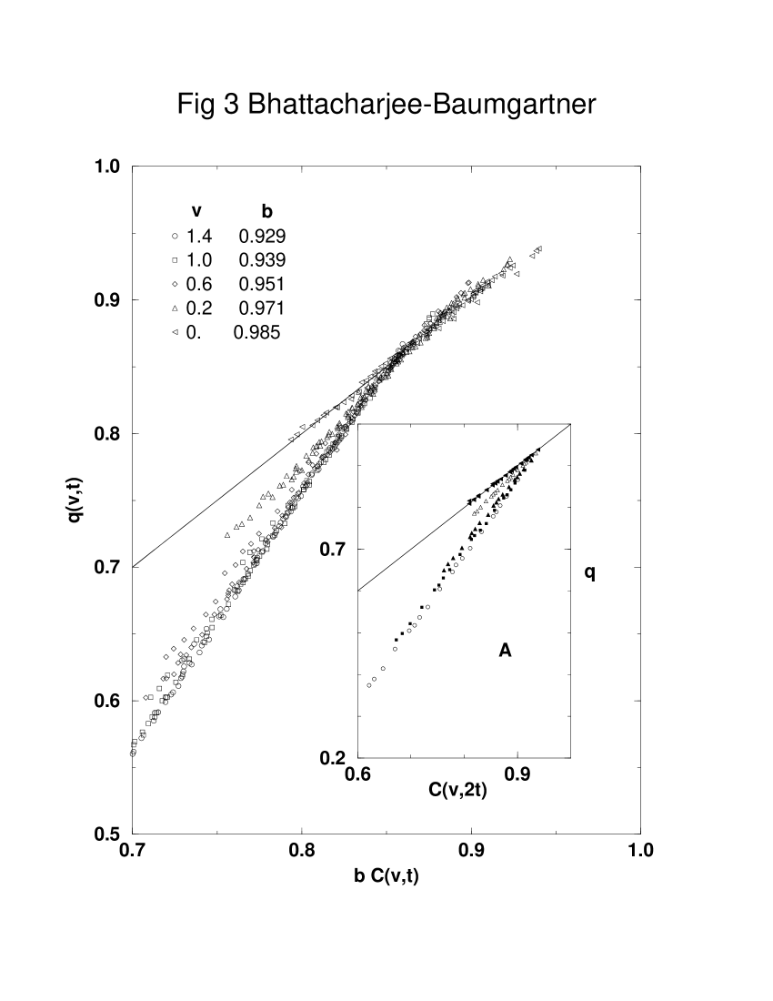
FIG. 3.: Plot of $q(v,t+t_{w})$ vs $bC(v,t+t_{w})$ for $t<t_{w}$, for various $v$ and $t_{w}$. Inset A shows the plot of $q(v,t+t_{w})$ vs $C(v,2t)$, for the largest $t_{w}$ for each $v$ (only a few data points are shown). The straight line is the equality line satisfied at $v=0$.

REFERENCES

- [1] R. M. Wartell and A. S. Benight, Phys. Rep. 126, 67 (1985).
- [2] Protein Folding ed. by T. E. Creighton (W. H. Freeman, NY 1992).
- [3] See, e.g., T. Halpin-Healy and Y. C. Zhang, Phys. Rept. 1995 and references therein.
- [4] A. Baumgärtner and M. Muthukumar, Adv. Chem. Phys. Vol XCIV, Ed by I. Prigogine and S. A. Rice (John Wiley, 1996)
- [5] K. Fischer and J. Hertz, Spin Glasses, (Cambridge, 1991)
- [6] M. Peyard and A. R. Bishop, Phys. Rev. Lett. 62, 2755 (1989).
- [7] L. C. E. Struik, Physical aging in amorphous polymers and other materials, (Elsevier, Houston, 1978).
- [8] L. Lundgren etal, Phys. Rev. Lett. 51, 911 (1983).
- [9] C. A. Angell, Science 267, 1924 (1995).
- [10] A more realistic situation would demand a random distribution of the contact energy. See, e.g., S. M. Bhattacharjee and S. Mukherji Phys. Rev. Lett. 70, 49 (1993).
- [11] E. Vincent et al., cond-mat/9607224, and references therein.
- [12] S. Mukherji, Phys. Rev E 50, R2407 (1994).
- [13] M. Kardar, Nucl. Phys. B 290, 582 (1988)
- [14] M. Mezard, J. Phys. (France) 51, 1831 (1990).
- [15] S. Mukherji and S. M. Bhattacharjee, Phys. Rev. E 53, R6002 (1996).
- [16] H. Kinzelbach and M. Lassig, Phys. Rev. Lett. 75, 2208 (1995).
- [17] D. S. Fisher, M. P. A. Fisher and D. A. Huse, Phys. Rev. B 43, 130 (1991).
- [18] A. Barrat, cond-mat/9701021
- [19] H. Yoshino, J. Phys. A 29, 1421 (1996).
- [20] See, e.g., A. Baumgärtner in “Applications of the Monte Carlo Method in Statistical Physics” ed. by K. Binder, Springer, Berlin, 1984.
- [21] The case of both ends free would correspond to annealed disorder because the chains then explore the whole space to choose the optimum position.
- [22] H. Rieger, Physica A 224, 267 (1996); J. Kisker etal, Phys. Rev B 1996.
- [23] L. V. Mikheev, B. Drossel and M. Kardar, Phys. Rev. Lett. 75, 1170 (1995).
- [24] K. P. N. Murthy and S. R. Shenoy, Phys. Rev A 36, 5087 (1987).
- [25] M. E. Fisher, J. Stat.Phys. 34, 667 (1984).
- [26] S. Mukherji and S. M. Bhattacharjee, J. Phys 26 L1139 (1993); 28, 4668 (1995) (E)