Numerical study of the transition of the four dimensional Random Filed Ising Model

Abstract

We study numerically the region above the critical temperature of the four dimensional Random Field Ising Model. Using a cluster dynamic we measure the connected and disconnected magnetic susceptibility and the connected and disconnected overlap susceptibility. We use a bimodal distribution of the field with $h_{R}=0.35T$ for all temperatures and a lattice size $L=16$. Through a least-square fit we determine the critical temperature at which the two susceptibilities diverge. We also determine the critical exponents $\gamma$ and $\overline{\gamma}$. We find the magnetic susceptibility and the overlap susceptibility diverge at two different temperatures. This is coherent with the existence of a glassy phase above $T_{c}$. Accordingly with other simulations we find $\overline{\gamma}=2\gamma$. In this case we have a scaling theory with two independent critical exponents.

1 Introduction

In the last few years the Random Field Ising Model [1], or RFIM, has attracted a lot of attention. Despite great efforts the critical behaviour of the model is still not clear. Both numerical and analytical studies have shown that in three dimensions at low temperature and sufficiently small field strength there is a transition from a disordered phase to a long range ordered phase. This result was first suggested by Imry and Ma [2]. They consider the possibility that the model could be split in clusters of dimension $L$. Through a direct comparison between ferromagnetic and random field energy they found a value of two for the lower critical dimension $d_{l}$. Subsequent arguments [3], based on perturbative expansion led to the result that the critical behaviour of the RFIM should be equivalent to that of the Ising model in two dimension fewer. This suggested a dimensional reduction of two so that, if this should be taken as a general rule, the lower critical dimension should be three instead of two. However, there is a rigorous proof, see Imbrie [4], that the lower critical dimension is two. It should be shown that, for a certain range of temperatures, the mean field equation has more than one solution; this is related to the fact that this model has a complex free energy landscape. This is essentially the reason why the dimensional reduction failed. An accurate numerical investigation of the mean field equation has been done by Guagnelli et al. [13] and successively by Lancaster et al. [12]. They have found that the mean field equation has more than one solution when the correlation length is still finite. In the spin glass [11] mean field theory we have a similar situation. It seems reasonable to use, in this case too, replica symmetry breaking theory such as that used by Parisi in that context. Mezárd et al. [8, 9], using RSB techniques and the SCSA approximation [10], have shown the existence of a region above the critical temperature in which there should be a “glassy” phase. In this case we have two different values of the critical temperature: one called $T_{c}$, which is the usual critical temperature of a ferromagnetic system, and another , called $T_{b}$ so that $T_{b}>T_{c}$, at which we have a transition from a paramagnetic phase to a “glassy” phase. In section two we first discuss the scaling theory of the model and then we introduce the concept of replica susceptibility. In section three we give a brief description of the algorithm used and then we show our results and conclusions in the last two section.

2 Theory

The RFIM is defined by the Hamiltonian

$$H_{rfim}=-J\sum_{<i,j>}\sigma_{i}\sigma_{j}-\sum_{i}h_{i}\sigma_{i}.$$ (1)

The variable $\sigma_{i}$ are Ising like spin and $h_{i}$ are independent random variable with mean $\left<h_{i}\right>_{av}=0$ and variance $\left<h_{i}^{2}\right>_{av}=h_{R}^{2}$. Typical distribution used is the Gaussian or bimodal distribution.

We first discussed the prediction of the scaling theory. Bray and Moore and independently, Fisher [5, 6] have proposed a scaling theory based on the assumption of a second order phase transition with a zero temperature fixed point. At $T=0$ for the correlation length, as usual, we expect a power law behaviour given by

$$\xi\propto t^{-\nu}.$$

In this case $t$ is such that

$$t=\frac{h_{R}}{J}-(\frac{h_{R}}{J})^{*},$$

where $(h_{R}/J)^{*}$ is the value of $h_{R}/J$ at the fixed point. The other relevant parameters are

$$\begin{array}[]{ccc}h&,&J.\end{array}$$

where $h$ is an uniform external field. Because for the RFIM the coupling constant is not fixed this yields to a change of the energy scale. In this case we obtain the modified hyperscaling relation

$$(2-\alpha)=(d-y)\nu,$$

where $y$ is the critical exponent related to $J$ in particular

$$J^{\prime}=b^{y}J.$$

Another difference with the Ising model is related to the correlation function. The presence of means over the quenched field causes the correlation function to have two different types of behaviour. We have a connected and a disconnected correlation function.

$$G_{con}(r)\equiv\overline{<\sigma_{0}\,\sigma_{r}>-<\sigma_{0}><\sigma_{r}>}=\frac{T}{r^{d-2+\eta}}\,g(r/\xi).$$ (2)

$$G_{dis}(r)\equiv\overline{<\sigma_{0}><\sigma_{r}>}=\frac{T}{r^{d-4+\overline{\eta}}}\,g^{\prime}(r/\xi).$$ (3)

This defines another critical exponent $\overline{\eta}$. The $\left<\dots\right>$ and the $\overline{(\dots)}$ denotes, respectively, the thermal average and the average over the different random field configuration. The other scaling relations are still valid in this case

$$\begin{array}[]{lcll}\alpha+2\,\beta+\gamma=2&,&\delta=\Delta/\beta&\dots\end{array}$$

In summary, we have eleven critical exponents and eight scaling relation. There seems to be a phase transition with three independent exponents. Schwartz and Soffer [7] have demonstrated the inequality

$$\overline{\eta}\leq 2\eta.$$ (4)

Numerical simulations [15] have suggested that (4) should be fulfilled like an equality. In this case we return to a two independent exponents transition.

If the transition is a spin glass like transition then the correct order parameter of the theory is the overlap

$$q=\overline{\left<\sigma_{i}\right>^{2}}.$$ (5)

In this case we are not interested in the magnetisation correlation function but in the replica correlation function. More in detailed we can define a magnetic susceptibility and an overlap susceptibility

$$\begin{array}[]{lcl}\overline{\chi(m)_{con}}&=&N[\overline{\langle m^{2}\rangle}-\overline{\langle m\rangle^{2}}]\\ \overline{\chi(m)_{dis}}&=&N[\overline{\langle m\rangle^{2}}]\\ \overline{\chi(q)_{con}}&=&N[\overline{\langle q^{2}\rangle}-\overline{\langle q\rangle^{2}}]\\ \overline{\chi(q)_{dis}}&=&N[\overline{\langle q\rangle^{2}}].\\ \end{array}$$ (6)

where $N$ is the volume of the lattice and we have a distinction between the connected and the disconnected parts. In this paper by means of Monte Carlo simulation we measured the four quantities in (LABEL:suscettive) in the region slightly above the critical temperature. In this way we are able to make a comparison between the susceptibility related to the magnetisation and that related to the overlap. If the three temperature transition scheme proposed in [9] is correct then the overlap and the magnetic susceptibility must diverge at two different temperatures.

3 The algorithm

The algorithm used to do the simulations is a generalisation of the cluster algorithm proposed by Wolff [17] for the Ising Model. According to the limited cluster flipped algorithm proposed by Newmann and Barkema [16] we have realised an algorithm capable of flipping more than one spin at a time. The algorithm is capable to forming clusters with a limited size. A Monte Carlo step consist of the two following points:

1. Build a cluster.

   • We choose a random site of the lattice. Then we choose, according to a certain distribution probability, the maximum size, $R$, of the cluster.

   • We add similarly oriented neighbouring spins. If the spin under consideration is within the allowed distance then we add it with probability $1-\exp{(-2\beta J)}$.

   • We repeat the above step until there are no more spins to add to the cluster.

2. Once the cluster is created we attempt to flip the spins inside it.

The cluster will be flipped with a probability factor proportional to the random field and to the number $s$ of spins which might have been added but which are found just outside the radius of the cluster. In detail we have

$$\left\{\begin{array}[]{ll}P_{flip}=\exp{(-2\beta J\,s)}&\mbox{if}\>m<0\\ P_{flip}=\frac{\exp{(-\beta m)}}{\exp{(\beta m)}}\,\exp{(-2\beta Js)}&\mbox{if}\>m>0\end{array}\right.$$

where $m=\sum_{i\in{C}}{h_{i}\sigma_{i}}$. As is explained in [16] this algorithm satisfies the conditions of ergodicity and detailed balance for the random field model. A Monte Carlo sweep is obtained when we have attempted to flip a number of clusters like the volume of the system.

We believe that for models such as the RFIM, this kind of dynamics is capable of strongly reducing the problem related to the dynamic slowing down approaching the critical temperature. Using a single spin flip dynamic a new configuration is obtained when we try to flip all the spins in the lattice. The probability of flipping a spin depends on the local fields through a term proportional to $p_{flip}(h)=\exp(-2\beta h_{i})$. It is possible that some spins are aligned to a large local field; in this case such spins are almost impossible to be flipped. Sometimes if we flip this “pinned” spin, the configuration obtained should be more probable than it was. When one of this spins is taken as a part of a cluster the effect of the field of such site should be rounded by the other fields in the cluster. In this case the procedure that realises the Monte Carlo dynamics is much more complicated than that of the Metropolis algorithm. Moreover, this kind of dynamics depends much from the contest. It is therefore necessary to spend a lot of time in optimising the algorithm.

4 Numerical results

Rieger and Young [14, 15] have carried out the most extensive Monte Carlo simulations in three dimensions in order to test the scaling relation validity. Using finite size scaling techniques they calculate all the critical exponents both with a Gaussian and with a bimodal probability distribution.

Making use of the cluster algorithm described in section 3 we carried out Monte Carlo simulation in order to search for numerical evidence of the existence of a “spin glass” like phase transition in the region above the critical temperature for a four dimensional lattice. To this end, at each Monte Carlo sweep, for each disorder realisation we measured the average magnetisation $\left<m\right>$ its square $\left<m^{2}\right>$, the average overlap $\left<q\right>$ and its square $\left<q^{2}\right>$; with $m=1/N\sum_{i=1}^{N}\sigma_{i}$ and $q=1/N\sum_{i=1}^{N}\sigma_{i}\tau_{i}$ where $\sigma_{i}$ and $\tau_{i}$ are two generic spins of two replica of the system. In this way we can calculate the four quantities given in (LABEL:suscettive). The two replica are such that they have the same realisation of the disorder. They will approach the equilibrium following two different markovian processes, in this case they can be considered independent. We performed the calculation using a four dimensional lattice of size $L=16$ with periodic boundary conditions. We have measured the quantities in (LABEL:suscettive) for $13$ different values of the temperature for each realisation of the disorder. Starting from a high temperature region we have cooled the system until ten percent of the critical temperature. The hardest region to simulate is the one near the critical temperature. For these temperatures the system takes a great deal of time to reach equilibrium. Near $T_{c}$ up to $250$ Monte Carlo sweeps were needed to balance the system. At temperatures $T$ sufficiently greater than $T_{c}$ the system balances very fast. In contrast, near $T_{c}$ the time needed to balance the system became too much long. For this reason if we took the same amount of Monte Carlo sweeps at each temperature we would waste time. We have used a range of temperature varying from $8.33$ to $5.97$ that correspond to $0.12\leq\beta\leq 0.1675$ where $\beta=1/T$.

Starting from $\beta=0.12$ we have cooled the system through the following rules

$$\beta = 0.12+(k-1)0.005,$$

$$k=1\ldots 8$$

$$\beta = 0.1575+(k-1)0.0025,$$

$$k=9\ldots 13.$$

In this way we have more points near $T_{c}$. At each temperature we have used a Monte Carlo sweep number ($\#MCs$) given by

$$\mbox{\#}MCs = 64k^{2}$$

$$k=1\ldots 13$$

A third of these have been used to balance the system and the rest to take the measurements. For $k=13$, i.e. near $T_{c}$, from the $10816\;\#MCs,$ the first $3605$ has been used to reach the equilibrium. This is an order greater than the calculated equilibration time. In this way, in the hardest region to simulate the thermal average there have been performed over more than $500$ uncorrelated measurements. The average over the disorder has been performed on $850$ samples. We need such a large number of samples because the quantities in (LABEL:suscettive) are highly non-self-averaging. For this reason the error caused by the disordered average is an order greater than that given by the thermal average. The random field has been chosen so that $h_{R}=0.35T$ for different temperatures. As was pointed out in [14] for greater values of $h_{R}/T$ the system is too difficult to balance and when the ratio is too small the system degenerates in the ferromagnetic model.

The quantity (LABEL:suscettive), near $T_{c}$ are well fitted by some power law of the temperature. Both for the the magnetic susceptibiliy and the overlap susceptibility we are sufficiently far from $T_{c}$ so we can neglect finite size effect. For the connected and disconnected magnetic susceptibility we used the following power law

$$\begin{array}[]{ccc}\overline{\chi(M)}&=&C(T-T_{c})^{-\gamma}\\ \overline{\chi(M)_{dis}}&=&C_{1}(T-T_{c})^{-\overline{\gamma}}.\end{array}$$ (9)

In figures (1) $1/\chi(m)_{con}$ and $1/\sqrt{\chi(m)_{dis}}$ are plotted against the temperature. It is clear from the figure that the two exponents $\gamma$ and $\overline{\gamma}$ are respectively slightly lower than one and two.

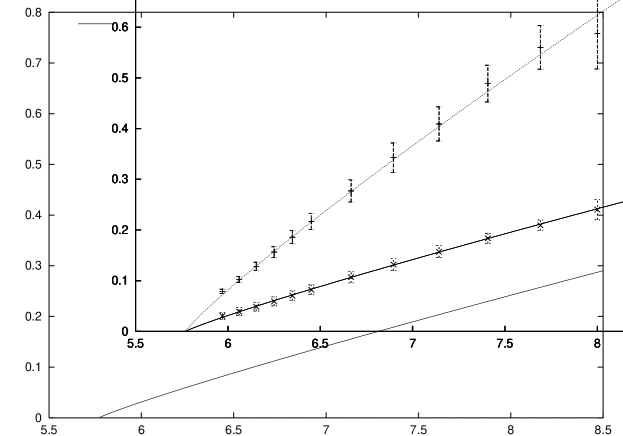
Figure 1: The full line and the dotted line represent the least-square fit results. The full line is the plot of $1/f(x)$ where $f(x)=8.9(T-T_{c})^{-0.94}$ and the dotted line is the plot of $1/f_{1}(x)^{(-1/2)}$ where $f_{1}(x)=12.1(T-T_{c})^{-1.91}$. The intersection with the abscissa gives the critical temperature.

The results of the least-square fit are such that

$$\begin{array}[]{ccc}T_{c}=5.72\pm 0.04&\gamma=0.94\pm 0.02&\overline{\gamma}=1.91\pm 0.08.\end{array}$$ (10)

The jacknife technique is used for the errors; the data are correlated since the same set of random fields is used at each temperature. According previous simulation [15] the Schwartz inequality [7] seems to be valid as an equality. Within the error bars we have $2\gamma=\overline{\gamma}$ that is

$$\overline{\eta}=2\eta.$$

Considering that $\overline{<Q^{2}>}\rightarrow 1$ when $T\rightarrow\infty$ we expect the connected overlap susceptibility to have a power behaviour given by

$$\begin{array}[]{ccc}\overline{\chi(Q)_{con}}&=&B(T-T_{b})^{-\omega}+D\end{array}$$ (11)

Because of the presence of the random field also the disconnected overlap susceptibility has a non vanishing term. We expect a power law behaviour given by

$$\begin{array}[]{ccc}\overline{\chi(Q)_{dis}}&=&B_{1}(T-T_{b})^{-\overline{\omega}}+D_{1}.\end{array}$$ (12)

We have reported in figure (2) the least-square fit result. As for the results in (10) the errors are calculated with the jacknife technique. We find

$$\begin{array}[]{ccc}T_{b}=5.88\pm 0.04&\omega=0.6\pm 0.1&\overline{\omega}=0.42\pm 0.05\end{array}$$ (13)

The (12) is valid near the critical temperature. It can be argued that the results found for the two critical temperatures, may be an artefact of the power-law behaviour used in (12). There could be a temperature drift in the non-singular term as the temperature is not too near from $T_{c}$. To take care of this effect we can add in (12) a linear term in the temperature vanishing near $T_{c}$. We can use a temperature dependence given by,

$$\begin{array}[]{ccc}\overline{\chi(Q)_{dis}}&=&B_{1}(T-T^{*})^{-\overline{\omega}}+D_{1}[1+D_{0}\frac{T-T^{*}}{T^{*}}].\end{array}$$ (14)

If we fix $T^{*}$ we can perform a four parameters fit. When $T^{*}=T_{c}$ the values of $\chi^{2}$ obtained is greater than that obtained in the previous fit. If we set $T^{*}=T_{b}$ we recover the results obtained using (12). In this case the temperature can be neglected and the results are well represented by the power law given in (12) The least-square fit results are reported in tabel 1.

Figure 2: Disconnected overlap susceptibility. The full line is the least-square fit result $f(x)=33(T-5.88)^{-0.42.}+41.$

	(12)	$T^{*}=T_{c}$	$T^{*}=T_{b}$
$B_{1}$	$33\pm 2$	$13.3\pm 0.9$	$32\pm 2$
$\overline{\gamma}$	$0.42\pm 0.02$	$1.09\pm 0.04$	$0.43\pm 0.02$
$D_{1}$	$41\pm 2$	$65\pm 1$	$43\pm 2$
$D_{0}$	$0$	$-0.22\pm 0.02$	$-0.03\pm 0.02$
$\chi^{2}$	$2.14$	$4.76$	$1.98$

Table 1: In the first column we have the least-square fit results obtained using the power law given in (12). The results in colunm two and three are obtained using the temperature dependence given in (14). In the last raw we have the values of $\chi^{2}$ calculated during the fit. The values in culomn one and three are almost equal. When $T^{*}=T_{b}$ we have $D_{0}\sim 0$ so that we can assume that (12) is a good approximation for all the temperatures used.

5 Conclusion

From the data analysis the overlap susceptibility and the magnetic susceptibility seems to diverge at two different points. It turns out that $T_{b}>T_{c}$. If this is the case the three transition scheme, obtained through RSB techniques, should be correct. A more extensive Monte Carlo simulations should be done near $T_{c}$, using finite size scaling techniques, in order to confirm the result obtained. It should be interesting as well to studing the overlap distribution probability in the region under $T_{b}$. Another result is given from the comparison between $\gamma$ and $\overline{\gamma}$. We find $\overline{\gamma}=2\gamma$, according to this result we have found one more scaling relation so that the independent critical exponents are two instead of three. In four dimension as well, the dimensional reduction is far from giving the correct result, in fact $\gamma=0.94$ is very far from $7/4$ which is a prediction of dimensional reduction.

References

- [1] D.P. Belanger, A.P. Young, J. Magn. Magn. Mater. 100,272 (1991).
- [2] Y. Imry, S.K. Ma, Phys. Rev. Lett. 35, 1399 (1975).
- [3] G. Parisi, N. Sourlas, Phys. Rev. Lett. 43, 744 (1979).
- [4] J. Z. Imbrie Phys. Rev. Lett. 53 (1984) 1747; J. Z. Imbrie Commun. Math. Phys. 98 (1985) 145;
- [5] A.J. Bray, M.A. Moore,J. Phys. C 18, L927 (1985).
- [6] D.S. Fisher, Phys. Rev. Lett. 56, 416 (1986).
- [7] M.Schwartz, A.Soffer J. Phys.,C 18, 1455 (1985). M.Schwartz J. Phys.,C 18, 135 (1985).
- [8] M.Mèzard, A.P. Young, Europhys. Lett., 18 (7), 653 (1992).
- [9] M. Mèzard, R. Monasson, preprint cond-mat/9406013 (1996).
- [10] A.J. Bray, Phys. Rev. Lett. 32, 1413 (1974).
- [11] M. Mézard, G. Parisi, M.A. Virasoro, “Spin Glass Theory and Beyond”, World Scientific (Singapore, 1992).
- [12] D. Lancaster, E. Marinari, G. Parisi preprint cond-mat/9412069 (1994).
- [13] M. Guagnelli, E. Marinari, G. Parisi preprint cond-mat/9303042 (1993).
- [14] H. Rieger, A.P. Young, J. Phys.,A 26, 5279 (1993).
- [15] H. Rieger, Phys. Rev.,B 52, 6659 (1995).
- [16] M.E.J. Newman, G.T. Barkema, Phys. Rev.,E 53, 393 (1996).
- [17] Ulli Wolff, Phys. Rev. Lett., 62, 361 (1989).