Numerical Simulations of the Dynamical Behavior of the SK Model

Abstract

We study the dynamical behavior of the Sherrington Kirkpatrick model. Thanks to the APE supercomputer we are able to analyze large lattice volumes, and to investigate the low $T$ region. We present a new and precise determination of the remnant magnetization and of its time decay exponent, of the energy time decay exponent, and we discuss aging phenomena in the model. We exclude validity of naive aging, and propose different options that fit the numerical data.

The study of the dynamical behavior of disordered (and complex) systems is receiving a large amount of attention (see for example [1, 2, 3, 4] and references therein). On one side this is because the study of dynamical behaviors can shed light on a large realm of new and interesting phenomena (aging is one of them). On the other side a reliable description of the amorphous glassy state will surely include a crucial, non-trivial dynamical behavior.

In many cases a full analytic computation is not yet feasible and many analytical results are based on conjectural grounds. Numerical simulations are here very useful in order to support the theoretical conjectures. Unfortunately a critical issue in the dynamics is the dependence of the times needed to reach equilibrium on the lattice size. This issue can be clarified only when both the size of the system is very large and the observation times are very long. This problem may be bypassed by considering the behavior of the infinite (practically very large) system as function of the (Monte Carlo) time.

This approach requires the study of very large systems. Unfortunately in the models that have been studied better, for which a full analytic solution for the static behavior is available, the time needed for executing one dynamical step increases severely with the lattice size. It grows as the lattice size $N$ to the second power, $N^{2}$ for the Sherrington-Kirkpatrick model (SK) [5], and as $N^{p}$ with $p\geq 3$ for the $p$-spin models. Faster simulations can be done for the diluted models, but in this case we do not known the static solution exactly. Moreover, given our lack of analytic control of the dynamic behavior, we cannot be completely sure that there are not some subtle differences among diluted and non diluted models.

Long range models may be classified into two different categories:

• In the first class of models (taken in the infinite volume limit) intensive quantities like the energy $E(t)$ or the magnetization $m(t)$ evolve toward their equilibrium values in the limit where $t\to\infty$.

• In the second category dynamical intensive quantities do not tend to their equilibrium values, and truly metastable states are present.

Such difference in the dynamical behavior is strong. It is believed that the models with a continuous replica symmetry breaking belong to the first category while models with a one step replica symmetry breaking belong to the second category.

The present investigation addresses this question in the case of the SK model [6]. The issue is very sensitive because some numerical investigations have suggested that the asymptotic properties of the SK model are different of the equilibrium one and in particular that the remnant magnetization is non zero also at infinite time [7] (that would also imply that the weak ergodicity breaking scenario cannot hold). One of the results of this note is to show that the value of the remnant magnetization is compatible with being zero in the infinite volume limit and that the SK model does belong to the first category we have described.

In the following we will show and discuss some of our numerical results. The main features that make these results relevant are that we have been able to work on large lattices and for low value of the temperature $T$. Our use of the APE-100 supercomputer [8] has been crucial to allow such large scale simulations. The fact that our program is truly parallelized (by dividing the spatial lattice among the different processors) makes possible to study very large lattices. Anyway the dynamics is still a sequential Metropolis one (we change one spin of a given system at the time). We also notice that since we are dealing with the infinite range mean field model obtaining, as in the code we used, an effective parallelization on a mesh with fixed connectivity is far from trivial.

In this note we will focus on the four main points we have been able to analyze:

1. We determine with good precision the time decay exponent of the magnetization.

2. We analyze the behavior of the remnant magnetization as a function of $N$.

3. We analyze the energy time decay exponent.

4. We discuss aging through the magnetization-magnetization time dependent correlation function.

First a few details about our simulations. We study the usual Sherrington-Kirkpatrick model [5, 9], with quenched couplings $J$ chosen from a Gaussian distribution. We have studied lattices of size $N=2088$, $4032$, $8064$ and $18432$, and $T=0.25$, $0.50$ and $0.75$ with a local Metropolis dynamics starting from a fully magnetized state (all spins set to $+1$ state). We study from $100$ to $200$ realizations of the quenched couplings for each $N$ value but for the largest one, where we have order $15$ samples. In each realization of the quenched disorder we have followed six copies of the system evolving independently (mainly to get a better computational efficiency). Runs have been $10000$ lattice sweeps long.

To fit our data we have used the Minuit library from Cernlib, and the jack-knife approach to compute statistical errors. The results we present here have been obtained by using large time windows for the fits.

The dynamical behavior of physical quantities in systems with relevant quenched disorder is usually expected to converge to the equilibrium values with power laws. The magnetization per spin on a lattice of size $N$ is expected to behave as

$$m^{(N)}(t)\simeq m_{\infty}^{(N)}+\tilde{m}^{(N)}t^{-\delta^{(N)}}\ ,$$ (1)

where the superscript $(N)$ (that we will omit in the following when we can do so without creating ambiguities) indicates that the parameters depend on the lattice size.

The previous formula needs a few comments. In any finite system the residual magnetization must eventually go to zero at infinite time. However we can distinguish at least two time scales. Let us consider for example the case of an unfrustrated system with two equal free energy states differing by a global spin reversal. At first the system will fall in one of the two equilibrium states, and on a much longer time scale the system will start to oscillate among the two different equilibrium states. Only in this second region of the time evolution the magnetization will become zero. If the ground states of the system are in some sense random, we may expect that from the central limit theorem the residual magnetization at the end of the first phase of the dynamics will be proportional to $N^{-\frac{1}{2}}$. A similar phenomenon for large, but not too large times is expected to take place here. The effective remnant magnetization is likely to be $N^{-\omega}$. While in an unfrustrated system $\omega=\frac{1}{2}$, the presence of a large number of equilibrium states suggests a smaller value of $\omega$ and our data are compatible with the value $\omega=\frac{1}{4}$ found close to $T_{c}$ for the SK model. The possibility $\omega=0$, i.e. of a non decay of the remnant magnetization with the size, is a priori possible, but it is not the one preferred by our data which are well compatible with an approach to equilibrium for all the quantities.

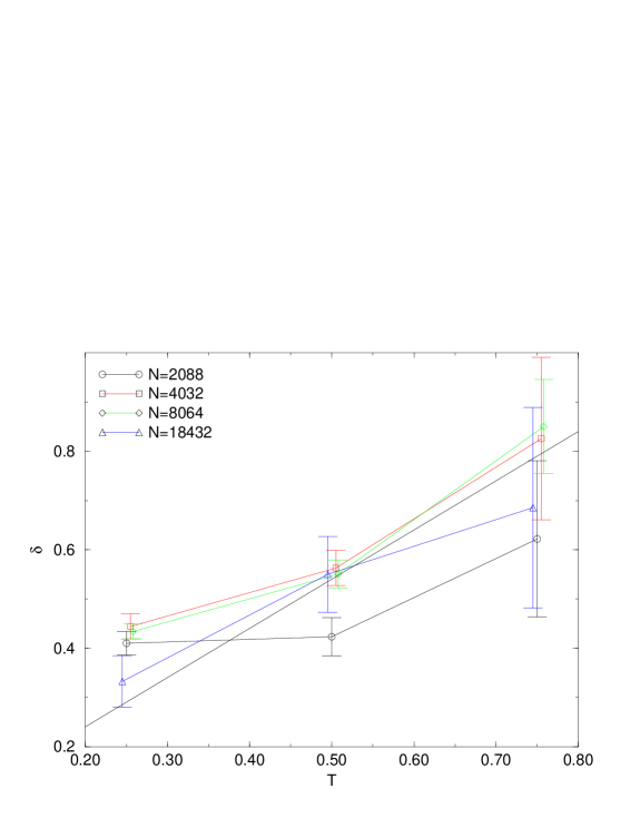
Figure 1: Magnetization decay exponent $\delta$ versus $T$ for different $N$ values.

In figure (1) we plot the exponent $\delta$ as a function of $T$ for the different $N$ values. Our data are not precise enough to detect a clear $N$ dependence of $\delta$ (only for the smallest lattice, $N=2088$ one can maybe read a systematic deviation). The straight line that goes through the figure is the line $\delta=\frac{T}{T_{c}}$: it fits very well the data, and indeed the fit is best on the larger lattice size, $N=18432$. We consider this plot as good evidence that

$$\delta(T)\simeq\frac{T}{T_{c}}\ .$$ (2)

The exponent $\delta$ is linear in $\frac{T}{T_{c}}$, and

$$\delta(T\to T_{c}^{-})=1$$ (3)

(for a discussion of the difference of this limit value and the limit $\delta(T\to T_{c}^{+})$ see the second of [1]). Our estimate is also compatible with the best estimate of [10], while the models defined on $\phi^{3}$ graphs (that is expected to have the same critical behavior of the SK model) seems to prefer a value $\delta(T)\simeq\frac{2T}{3T_{c}}$ [11].

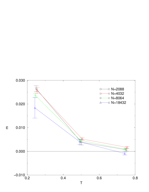
Figure 2: The remnant magnetization versus $T$ for different $N$ values.

We plot our best estimate for the remnant magnetization as a function of $T$ for different $N$ values in figure (2). The $N$ dependence of the data is very weak. When assuming a power decay one finds that the data are fully compatible with the power $\frac{1}{4}$, as discussed in the second of [1]. It is clear from our data that a constant behavior, with a non-zero residual magnetization, cannot be excluded.

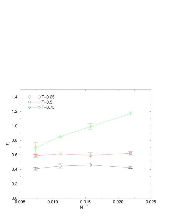
Figure 3: The energy time decay exponent versus $N^{-1/2}$ for different $T$ values.

Our third result concerns the energy time decay exponent. In figure (3) we show it versus the inverse square root of the volume. At low $T$ we get an $N$-independent estimate, with a clear dependence over $T$ (we get $.4$ at $T=.25$ and $.6$ at $T=.5$). At $T=.75$ we seem to have a strongly $N$-dependent result. Even if in this case it is not easy to be sure, the behavior of the power exponent is again compatible with a linear dependence on $T$.

Our last results concern aging. We have measured the two time spin-spin correlation function

$$C(t_{w},t_{w}+t)\equiv\frac{1}{N}\overline{\langle\sum_{i}\sigma_{i}(t_{w})\sigma_{i}(t_{w}+t)\rangle}\ ,$$ (4)

always starting from random initial conditions. Our simulations were performed at $T=.5T_{c}$, with “lattice size” $N=4096$ and $16$ independent samples with $6$ replicas each.

The simplest scenario one can think about is naive aging, i.e.

$$C(t_{w},t_{w}+t)=f(\frac{t}{t_{w}})\ ,$$ (5)

in the region where both $t$ and $t_{w}$ are large.

Our results for $C$ are displayed in figure (4). Although the data are in some very rough agreement with a naive aging behavior there are strong systematic corrections which obviously modify the functional form of (5). Naive aging is not satisfied in the Sherrington-Kirkpatrick model. The type of violations of naive aging are similar to those observed in real experiments: the function $C(t_{w},t_{w}+t)$ at fixed $s\equiv\frac{t}{t_{w}}$ decreases (increases) when $t_{w}$ increases for $s<1$ (for $s>1$).

In naive aging one assumes that the time scale of relaxation at $t_{w}$ scales as $t_{w}$ and this assumption is not correct in the approach of [12] and [2, 3]. One can take one of many different attitudes.

The first possibility is that naive aging is not correct, and we decide to use some phenomenological corrections to it. In this case a different form of scaling may be expected. The most popular assumption is interrupted aging [12]. It corresponds to assume that

$$C(t_{w},t_{w}+t)=f(\frac{t}{t_{w}}^{1+\mu})\ .$$ (6)

The introduction of the power correction $\mu$ may help to fit the data at large $\frac{t}{t_{w}}$ but it does not improve the situation at small $\frac{t}{t_{w}}$ and spoils the agreement of aging at $\frac{t}{t_{w}}\simeq 1$. It seems that this correction is not very useful here. Moreover there is no theoretical justification for interrupted aging in this context.

Another possibility, natural in the contest of [2, 3] is to assume that

$$C(t_{w},t_{w}+t)=f(\frac{\ln(t+t_{w})}{\ln(t_{w})})\ .$$ (7)

We have plotted our data for $C(t_{w},t_{w}+t)$ versus $\ln(t+t_{w})/\ln(t_{w})$ in figure (5). This change of the scaling law definitely improves the situation, so this is a possible solution to the problem. It is interesting to note that in this version of the scaling form we have that

$$\lim_{t_{w}\to\infty}C(t_{w},\lambda t_{w})$$ (8)

goes to a value independent on $\lambda$, which can be therefore identified with $q_{EA}$. Obviously in this case the function $f$ will be discontinuous when its argument is equal to one. We can also say that the time for reaching a given value of $C<q_{EA}$ is given by

$$t=t_{w}^{\gamma(C)}$$ (9)

where the function $\gamma$ is related to the function $f$. For large values of $t_{w}$ the value of $C$ that can be reached after the time $t$ and after $\lambda t$ do coincide. In this way the ultrametricity of the configurations is satisfied also in the dynamics (as it should be): for example it implies that if in a given time we can go at distance $1-C$ from a given configurations, we can arrive always at the same distance if we double the time. This would be the scenario that is in better agreement with the existing theoretical computations [3].

The last possibility is that naive aging is asymptotically correct, but there is a correction to it which vanishes as a negative power of time. The rational for this choice is that we know (as we shall see later) that some power corrections to scaling are necessarily present at small $t$.

Here we explore if this third possibility is compatible with our numerical data. We note that in the region where $t\ll t_{w}$ we should have

$$C(t_{w},t_{w}+t)=q_{EA}+At^{-\alpha}\ .$$ (10)

The exponent $\alpha$ is a function of $T$; it is equal to $0.5$ at the critical temperature and it decreases to a smaller value when $T$ decreases (it has been estimated to be equal to $0.36$ at zero temperature [13]). As far as the value of $\alpha$ is not too large (and it is certainly much smaller than $0.36$ for three dimensional spin glasses, i.e. close to $0.06$) the corrections to the scaling law cannot be easily neglected.

The simplest modification to the naive aging prediction which is compatible with the previous equation is:

$$C(t_{w},t_{w}+t)=f_{0}(\frac{t}{t_{w}})+t^{-\alpha}f_{1}(\frac{t}{t_{w}})\ ,$$ (11)

where the two functions $f_{0}(s)$ and $f_{1}(s)$ are not divergent in the limit $s\to 0$. In principle also the exponent $\alpha$ could be a function of $s$, but for simplicity we assume that it is a constant.

We have fitted the data using equation (11). The best value of $\alpha$ we find is $0.2$, which is a factor two smaller that the theoretical predictions. The origin of this discrepancy is not clear (possible reasons are finite volume effects, a crossover behavior at $s=0$, a strong $s$ dependence of $\alpha$). If we stick to our best value $\alpha=0.2$ we obtain the functions $f_{0}(s)$ and $f_{1}(s)$ displayed in figures (6) and (7). In this way we estimate a value of $q_{EA}$ close to $0.75$, which is slightly different from the theoretical value $\simeq 0.6$. Also in this case the origins of this discrepancy are not clear.

In order to exhibit the quality of our best fits we show in figure (8) the quantity $C(t_{w},t_{w}+t)-f_{1}(\frac{t}{t_{w}})\ t^{-\alpha}$. Here, at the expense of having introduced an extra function, the data seem to collapse well on a single curve. We also plot the same quantity for a different value of $\alpha$, to show that in this case the collapse is not as good.

The main difference among the behavior of (11) and the one of (7) is that in the case of (11) $\lim_{t_{w}\to\infty}C(t_{w},t_{w}\cdot(1+s))$ is a non-trivial function of $s$, while in the case of (7) it does not depend on $s$. The scaling (7) is indeed in agreement with a picture where the barriers for reaching a value $\overline{q}$ of the overlap strongly depend on $\overline{q}$.

Longer runs on larger lattices will be able to improve our understanding of the situation. We believe that understanding details of the aging pattern is important, and that these results are a first step toward this interesting goal.

Figure 4: $C(t,t_{w})$ as a function of $\frac{t}{t_{w}}$ for different $t_{w}$ values (from 8 to 32768). $T=0.5T_{c}$.

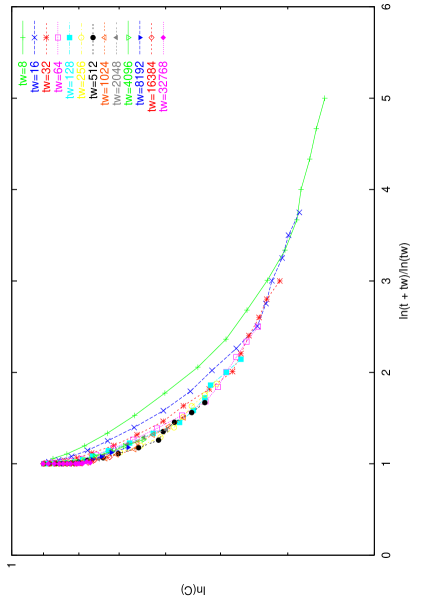
Figure 5: $\ln C(t_{w},t_{w}+t)$ as a function of $\ln(t+t_{w})/\ln(t_{w})$. $T=0.5T_{c}$.

Figure 6: Fitted $f_{0}$ as a function of $\frac{t}{t_{w}}$ for $\alpha=0.2$. $T=0.5T_{c}$.

Figure 7: Fitted $f_{1}$ as a function of $\frac{t}{t_{w}}$ for $\alpha=0.2$. $T=0.5T_{c}$.

Figure 8: $C(t_{w},t_{w}+t)-f_{1}(\frac{t}{t_{w}})t^{-\alpha}$ for $\alpha=0.2$ and $\alpha=0.45$. $T=0.5T_{c}$.

References

- [1] G. Parisi, cond-mat/9701015; G. Parisi, P. Ranieri, F. Ricci-Tersenghi and J. Ruiz-Lorenzo, cond-mat/9702039; E. Marinari, G. Parisi, F. Ricci-Tersenghi and J. Ruiz-Lorenzo, cond-mat/9710120.
- [2] S. Franz and M. Mézard, Europhys. Lett. 26 (1994) 209.
- [3] L. Cugliandolo and J. Kurchan, Phil. Mag. 71 (1995) 501; J. Phys A: Math. Gen. 27 (1994) 5749.
- [4] A. Baldassarri, cond-mat/9607162; H. Yoshino, cond-mat/9612071.
- [5] D. Sherrington and S. Kirkpatrick, Phys. Rev. Lett. 35 (1975) 1792; S. Kirkpatrick and D.Sherrington, Phys. Rev. B 17 (1978) 4384.
- [6] G. Parisi and F. Ritort, J. Phys. 3 (1993) 969.
- [7] W. Kinzel, Phys. Rev. B 33 (1986) 5086; R. D. Henkel and W. Kinzel, J. Phys. A: Math. Gen. 20 (1987) L727; W. Kinzel J. Phys. C: Solid State Phys. 21 (1988) L381.
- [8] A. Bartoloni et al., Int. J. High Speed Comp. 5 (1993) 637; Int. J. Mod. Phys. C4 (1993) 955; Int. J. Mod. Phys. C4 (1993) 969.
- [9] M. Mézard, G. Parisi and M. A. Virasoro, Spin Glass Theory and Beyond (World Scientific, Singapore 1987).
- [10] G. Ferraro, cond-mat/9407091.
- [11] C. Baillie, D. A. Johnston, E. Marinari and C. Naitza, cond-mat / 9606194, J. Phys. A: Math. Gen. 29 (1996) 6683.
- [12] J.-P. Bouchaud, J. Physique (France) 2 (1992) 1705.
- [13] H. Sompolinsky and A. Zippelius, Phys. Rev. Lett. 47 (1981) 359; Phys. Rev. B 25 (1982) 6860; Phys. Rev. Lett. 50 (1983) 1297; P. Biscari, Europhys. Lett. 6(1989) 47.