The Hubbard model in the two-pole approximation

Abstract

The two-dimensional Hubbard model is analyzed in the framework of the two-pole expansion. It is demonstrated that several theoretical approaches, when considered at their lowest level, are all equivalent and share the property of satisfying the conservation of the first four spectral momenta. It emerges that the various methods differ only in the way of fixing the internal parameters and that it exists a unique way to preserve simultaneously the Pauli principle and the particle-hole symmetry. A comprehensive comparison with respect to some general symmetry properties and the data from quantum Monte Carlo analysis shows the relevance of imposing the Pauli principle.

I Introduction.

The Hubbard model [1] plays a key role [2] in the theoretical analysis of highly correlated electron systems and in the last years many works have been devoted to its study. The relevance of the model is that contains as a main ingredient a competition between the band energy, which tends to distribute the electrons throughout the entire crystal, and the repulsive electron-electron interaction which tends to localize the electrons on the lattice sites. Although the model is oversimplified and in spite of a very intensive study, both analytical and numerical, exact solutions exist only in one and infinite dimensions. For finite dimensions greater than one the study is far from being completed and more analysis is required. Many techniques and various approximation schemes have been formulated; among them we recall the Hubbard I approximation [1], the slave boson method [3-5], the non-crossing approximation [6-8], the $d_{\infty}$ method [9-12], the projection operator method [13- 18], the method of equation of motion [19-21], the spectral density approach [22-24], the composite operator method [25-31].

When the lowest level of approximation is considered, many methods [1, 13-31], though based on different schemes, give an equivalent framework of calculation, where the spectral function of the single-particle propagator is approximated by a two-pole expansion. A common feature of all these methods is that a self-consistent procedure is necessary in order to calculate some parameters which appear in the expression of the spectral function. As a consequence, although many methods seems to be equivalent, remarkable differences arise, according to the different adopted procedures.

The purpose of this work is to analyze various methods and compare the different predictions with respect to some general symmetry properties of the model and with respect to the numerical data obtained by quantum Monte Carlo (qMC) techniques.

II The Model.

The Hubbard model is defined by

$$H=\sum_{ij}t_{ij}c^{\dagger}(i)c(j)+U\sum_{i}n_{\uparrow}(i)n_{\downarrow}(i)-\mu\sum_{i}c^{\dagger}(i)c(i)$$ (1)

The first term is a kinetic term that describes the motion of the electrons among the sites of the Bravais lattice, defined by the vector set $\{{\rm\bf R}_{i}\}$. For a two-dimensional squared lattice and by restricting the analysis to first nearest neighbors, the hopping matrix $t_{ij}$ has the form

$$t_{ij}=-4t\alpha_{ij}=-4t{1\over N}\sum_{{\rm\bf k}}e^{i{\rm\bf k}\cdot({\rm\bf R}_{i}-{\rm\bf R}_{j})}\alpha({\rm\bf k})$$ (2)

$$\alpha({\rm\bf k})={1\over 2}\left[\cos(k_{x}a)+\cos(k_{y}a)\right]$$ (3)

$a$ being the lattice constant. In addition to the band term, the model contains an interaction term which approximates the interaction among the electrons. In the simplest form of the Hubbard model, the interaction is between electrons of opposite spin on the same lattice site; the strength of the interaction is described by the parameter $U$. Various generalizations of the model take into account hopping between second nearest neighbors and intersite interactions. $c(i)$, $c^{\dagger}(i)$ are annihilation and creation operators for $c$-electrons at site $i$ in the spinor notation

$$c={c_{\uparrow}\choose c_{\downarrow}}\qquad c^{\dagger}=\left(c^{\dagger}_{\uparrow}\quad c^{\dagger}_{\downarrow}\right)$$ (4)

$n_{\sigma}(i)=c^{\dagger}_{\sigma}(i)c_{\sigma}(i)$ is the number operator of electrons with spin $\sigma=(\uparrow,\downarrow)$ at the $i$-th site. $\mu$ is the chemical potential and is introduced in order to control the band filling $n=\langle c^{\dagger}(i)c(i)\rangle$. By varying the ratio $U/t$, the particle number $n$ and the temperature $T$, it is believed that the Hubbard model is capable to describe many properties of strongly correlated fermion systems [2].

The field $c(i)$ satisfies the equation of motion

$$i{\partial\over\partial t}c(i)=-\mu c(i)+\sum_{j}t_{ij}c(j)+Un(i)c(i)$$ (5)

where the composite field

$$\eta(i)=n(i)c(i)$$ (6)

appears. By means of the Hamiltonian (2.1) one can derive the equation of motion for the new field

$$i{\partial\over\partial t}\eta(i)=-(\mu-U)\eta(i)+4t\pi(i)$$ (7)

where a higher order composite field appears

$$\pi(i)=\sum_{j}\alpha_{ij}\left[{1\over 2}\sigma^{\mu}n_{\mu}(i)c(j)+c(i)c^{\dagger}(j)c(i)\right]$$ (8)

In Eq. (2.8) we introduced the charge ($\mu=0$) and spin ($\mu=1,2,3$) density operator

$$n_{\mu}(i)=c^{\dagger}(i)\sigma_{\mu}c(i)$$ (9)

with the notation

$$\sigma_{\mu}=(1,\vec{\sigma})\qquad\sigma^{\mu}=(-1,\vec{\sigma})$$ (10)

$\sigma_{k}$ being the Pauli matrices.

In order to close the infinite hierarchy of equations of motion some truncation is necessary. One procedure, common to various methods, is to choose a basis of operators $\{\Psi(i)\}$ and linearize the equation of motion as

$$i{\partial\over\partial t}\Psi(i)=\sum_{j}\varepsilon_{ij}\Psi(i)$$ (11)

where the eigenvalue or energy matrix is self-consistently calculated by means of the equation

$$\varepsilon_{ij}=\langle[\Psi(i),H],\Psi^{\dagger}(j)]_{\pm}\rangle/\langle[\Psi(i),\Psi^{\dagger}(j)]_{\pm}\rangle$$ (12)

The symbol $[\ldots]_{\pm}$ denotes equal-time anticommutator or commutator, in dependence of the statistics of the set $\{\Psi(i)\}$. The rank of the energy matrix is equal to the number of components of $\Psi(i)$. It should be noted that $\varepsilon_{ij}$ may extend over several lattice points, according to the choice of the basis $\{\Psi(i)\}$. Different choices for the basis $\{\Psi(i)\}$ can be taken. The mean field approximation corresponds to the choice $\Psi=c$. In Table I we summarize some choices used in various works.

Refs. 1,20,21	$\displaystyle\Psi=\left({c\atop\eta}\right)$
Ref. 18	$\displaystyle\Psi=\left({c\atop\eta-\langle n/2\rangle c}\right)$
Refs. 17,26	$\displaystyle\Psi=\left({\xi\atop\eta}\right)$

TABLE I.:  

The composite operator $\xi(i)$ is defined as

$$\xi(i)=c(i)-\eta(i)=[1-n(i)]c(i)$$ (13)

It is easy to show by direct calculations of the energy matrices that all basis are equivalent and they all give place to the same linearized equations of motion. By considering a paramagnetic ground state, the thermal retarded Green’s function

$$S_{\Psi\Psi}(i,j)=\langle R[\Psi(i)\Psi^{\dagger}(j)]\rangle$$ (14)

after the Fourier transformation, has the following expression

$$S_{\Psi\Psi}({\rm\bf k},\omega)=\sum^{2}_{i=1}{\sigma^{(i)}_{\Psi\Psi}({\rm\bf k})\over\omega-E_{i}({\rm\bf k})+i\eta}$$ (15)

The energy spectra $E_{i}({\rm\bf k})$ are given by

$$E_{1}({\rm\bf k})=R({\rm\bf k})+Q({\rm\bf k})\qquad E_{2}({\rm\bf k})=R({\rm\bf k})-Q({\rm\bf k})$$ (16)

where

$$R({\rm\bf k})={1\over 2}\left[-2\mu+U\right]-{1\over 2I_{1}I_{2}}\left[m({\rm\bf k})+8t\alpha({\rm\bf k})I_{1}I_{2}\right]$$ (17)

$$Q({\rm\bf k})={1\over 2}\sqrt{g^{2}({\rm\bf k})+{4m^{2}({\rm\bf k})\over I_{1}I_{2}}}$$ (18)

and the following notation has been used

$$I_{1}=1-n/2\qquad I_{2}=n/2$$

$$m({\rm\bf k})=4t\left[\Delta+\alpha({\rm\bf k})(p-I_{2})\right]$$ (19)

$$g({\rm\bf k})=-U+{1-n\over I_{1}I_{2}}m({\rm\bf k})$$

The parameters $\Delta$ and $p$ describe a constant shift of the bands and a bandwidth renormalization, respectively. They are static intersite correlation functions defined as

$$\Delta\equiv\langle\xi^{\alpha}(i)\xi^{\dagger}(i)\rangle-\langle\eta^{\alpha}(i)\eta^{\dagger}(i)\rangle$$ (20)

$$p\equiv{1\over 4}\langle n^{\alpha}_{\mu}(i)n_{\mu}(i)\rangle-\langle\left[c_{\uparrow}(i)c_{\downarrow}(i)\right]^{\alpha}c^{\dagger}_{\downarrow}(i)c^{\dagger}_{\uparrow}(i)\rangle$$ (21)

The notation $c^{\alpha}(i)$ stands to indicate the field $c$ on the first neighbor sites:

$$c^{\alpha}(i)=\sum_{j}\alpha_{ij}c(j)$$ (22)

The explicit expressions of the spectral functions $\sigma^{(i)}_{\Psi\Psi}({\rm\bf k})$ are given by [26]

$$\sigma^{(1)}_{\xi\xi}({\rm\bf k})={I_{1}\over 2}\left[1+{g({\rm\bf k})\over 2Q({\rm\bf k})}\right]\qquad\qquad\sigma^{(2)}_{\xi\xi}({\rm\bf k})={I_{1}\over 2}\left[1-{g({\rm\bf k})\over 2Q({\rm\bf k})}\right]$$

$$\sigma^{(1)}_{\xi\eta}({\rm\bf k})={m({\rm\bf k})\over 2Q({\rm\bf k})}\qquad\qquad\sigma^{(2)}_{\xi\eta}({\rm\bf k})=-{m({\rm\bf k})\over 2Q({\rm\bf k})}$$ (23)

$$\sigma^{(1)}_{\eta\eta}({\rm\bf k})={I_{2}\over 2}\left[1-{g({\rm\bf k})\over 2Q({\rm\bf k})}\right]\qquad\qquad\sigma^{(2)}_{\eta\eta}({\rm\bf k})={I_{2}\over 2}\left[1+{g({\rm\bf k})\over 2Q({\rm\bf k})}\right]$$

The spectral functions relative to other basis can be obtained from (2.23) by recalling that $c(i)=\xi(i)+\eta(i)$.

Straightforward calculations, reported in Appendix B, show that the first four momenta

$$M^{(n)}({\rm\bf k})=\int^{+\infty}_{-\infty}d\omega A({\rm\bf k},\omega)\omega^{n}$$ (24)

of the electron spectral density

$$A({\rm\bf k},\omega)=-{1\over\pi}ImS_{cc}({\rm\bf k},\omega)=\sum^{2}_{i=1}\sigma^{(i)}_{cc}({\rm\bf k})\delta\left[\omega-E_{i}({\rm\bf k})\right]$$ (25)

satisfies the exact relations

$$M^{(n)}({\rm\bf k})=F.T.\langle\left\{\left(i{\partial\over\partial t}\right)^{n-p}c(i),\left(-i{\partial\over\partial t^{\prime}}\right)^{p}c^{\dagger}(j)\right\}_{E.T.}\rangle\ ,\quad 0\leq p\leq n$$ (26)

where $F.T.$ denotes the Fourier transform. Then, there is a complete equivalence between the scheme of calculation traced above and the spectral density approach [23], when the two-pole approximation is considered.

Summarizing, when the lowest order is considered all various methods [1, 13-31] are equivalent and they all correspond to a two-pole approximation with the same expression for the spectral function. The correspondence with the notation of Refs. 20 and 18 is given by

$$I_{1}I_{2}W({\rm\bf k})=I_{1}I_{2}\left[W_{0}+W_{1}({\rm\bf k})\right]=-I_{1}I_{2}\mu-4t\Delta+4t\alpha({\rm\bf k})\left[I^{2}_{2}-p\right]$$ (27)

However, the scheme is not complete unless the self-consistent procedure is defined. The spectral functions contain three unknown parameters, $\mu$, $\Delta$, and $p$ very different results are obtained according to the methods used to calculate them. This will be discussed in the next Sections.

III Self-consistent equations.

In Section 2 the energy matrix and therefore the properties of the basic fields $\{\Psi\}$ have been fixed by means of Eq. (2.12). However, as we have seen, this constrain does not fix in a unique way the dynamics; the parameters $\mu$, $\Delta$, and $p$ remain to be determined and more conditions are required.

One constrain common to all methods is given by the requirement that the particle number is an external parameter, fixed by the boundary conditions. Then, the following self-consistent equation must be satisfied:

$$n=2\left[1-C_{cc}\right]$$ (28)

where the correlation function $C_{cc}$ is defined in (A.8). We need two more conditions. In Hubbard I approximation [1] a simple factorization procedure is used for the two-particle Green’s function. Then, from the definitions (2.20) and (2.21) one obtains the expressions

$$\Delta = 0$$ (29)

$$p = {n^{2}\over 4}$$ (30)

However, Eq. (3.2) is not consistent with the present scheme of calculation. The parameter $\Delta$ is directly connected to the single-particle Green’s function, and from the definition (2.20) one can immediately derive the self-consistent equation

$$\Delta=C^{\alpha}_{\xi\xi}-C^{\alpha}_{\eta\eta}$$ (31)

where the time-independent correlation functions are defined by Eq. (A.6). The parameter p plays an important role since it is related to neighboring correlations of the charge, spin and pair. An accurate determination of this parameter is very important; as it will be shown in the next Sections, different methods of computing p give rise to very different physical solutions.

In the original work by Roth [20] and in subsequent works [18, 21] the parameter p has been calculated by means of the equation of motion in the linearized form (2.11). This procedure leads to the following relation

$$p=I^{2}_{2}-{(2-\beta\over I_{1}(1-\beta^{2})}\left[C^{\alpha}_{cc}(C^{\alpha}_{cc}-C^{\alpha}_{c\eta})+C^{\alpha}_{c\eta}(I^{-1}_{2}C^{\alpha}_{c\eta}-C^{\alpha}_{cc})\right]-{1\over I_{1}I_{2}(1-\beta)}C^{\alpha}_{c\eta}(C^{\alpha}_{cc}-C^{\alpha}_{c\eta})$$ (32)

where

$$\beta={I_{2}-C^{\alpha}_{\eta\eta}-I^{2}_{2}\over I_{1}I_{2}}$$ (33)

and the correlation functions $C^{\alpha}_{cc}$, $C^{\alpha}_{c\eta}$ are given by Eq. (A.8).

In the Composite Operator Method we adopt a different procedure to calculate the parameter $p$. This quantity is not expressed in terms of the single-particle propagator, and there is some freedom in its determination. In COM we take advantage of this freedom and we fix the parameter $p$ in such a way that the Hilbert space has the right properties to conserve the relations among matrix elements imposed by symmetry laws.

There is a wide agreement that the unusual and somehow unexpected properties observed in the new class of materials are due to the presence of a high correlation among the electrons. If the electron interaction is the key to understand these materials, then it is very crucial that the symmetry required by the Pauli principle is correctly treated. A convenient way to take care of the Pauli principle is to operate in the representation of second quantization where the Pauli principle manifests through the algebra. However, algebra is only one ingredient; physical quantities are expressed in terms of expectation values of operators and a suitable choice of the Hilbert space must be made. Physical laws, expressed as algebraic relations among the observables, manifest at the level of observation as relations among matrix elements.

In a physics dominated by a high correlation among the electrons, we feel that greater attention should be dedicated to the conservation of the Pauli principle. It is well known that in most of the approximation schemes this symmetry is violated [19], and some alternative schemes should be considered. The Pauli principle requires that

$$\xi_{\sigma}(i)\eta^{\dagger}_{\sigma}(i)=c_{\sigma}(i)\left[n_{-\sigma}(i)-n^{2}_{-\sigma}(i)\right]c^{\dagger}_{\sigma}(i)=0$$ (34)

At level of matrix elements, this condition requires that

$$C_{\xi\eta}=\langle\xi(i)\eta^{\dagger}(i)\rangle=0$$ (35)

By recalling the expression (A.5) for the correlation function $C_{\xi\eta}$ and by means of Eqs. (A.7) and (2.19), we easily obtain the following self-consistent equation for the parameter $p$

$$p={n\over 2}-\Delta{F_{0}\over F_{1}}$$ (36)

where the quantities $F_{0}$ and $F_{1}$ are defined by (A.7).

Summarizing, the adopted self-consistent procedures are based on the use of Eqs. (3.1), (3.4), (3.5) in the Roth’s method, and of Eqs. (3.1), (3.4), (3.9) in the COM. It should be noted that the self- consistent equations are all coupled, so that a different choice for the third equation will have influence also on the first two equations. In particular, when the Pauli condition (3.8) is not satisfied, there is an ambiguity in writing the first-self consistent equation (3.1). In the next section we shall discuss and compare the different results which arise, due to the use of different self-consistent schemes.

IV The Pauli principle and the particle-hole symmetry.

The conservation of the Pauli principle in the Roth’s method is studied in Fig. 1, where the normalized Pauli amplitude $B_{N}=\langle\xi(i)\eta^{\dagger}(i)\rangle/\langle\eta(i)\eta^{\dagger}(i)\rangle$ is reported vs $n$ for various values of $U$.

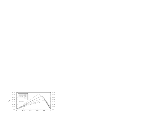
FIG. 1.: The normalized Pauli amplitude in the Roth’s method $B_{N}=\langle\xi(i)\eta^{\dagger}(i)\rangle/\langle\eta(i)\eta^{\dagger}(i)\rangle$ is given as a function of the filling for various values of the potential intensity $U$.

We see that in the Roth scheme the Pauli principle is satisfied only in the cases $n=0$ and $n=1$. Also, the deviations increase by decreasing U, showing that the non interacting case [i.e. $U=0$] is not reproduced in this formulation. At the contrary; the Pauli principle is recovered in the limit $U\rightarrow\infty$ for any value of $n$.

As a consequence of the fact that the Pauli principle is not satisfied also the particle-hole symmetry is violated. The Hubbard Hamiltonian has an important property of symmetry: it remains invariant under the particle-hole transformation

$$c_{\sigma}(i)\to(-1)^{i}c^{\dagger}_{\sigma}(i)$$ (37)

By noting that under the transformation (4.1)

$$\begin{array}[]{ll}c^{\dagger}c\to 2-c^{\dagger}c&c^{\dagger}\sigma_{3}c\to-c^{\dagger}\sigma_{3}c\\ \xi\to\eta^{\dagger}&\eta\to\xi^{\dagger}\end{array}$$ (38)

the self-consistent parameters scale as

$$\mu(2-n) = U-\mu(n)$$ (39)

$$\Delta(2-n) = -\Delta(n)$$ (40)

$$p(2-n) = p(n)+(1-n)$$ (41)

Then, it is easy to derive the following relations

$$\begin{array}[]{ll}C_{\xi\xi}(2-n)=C_{\xi\xi}(n)-(1-n)&C^{\alpha}_{\xi\xi}(2-n)=C^{\alpha}_{\eta\eta}(n)\\ C_{\xi\eta}(2-n)=-C_{\xi\eta}(n)&C^{\alpha}_{\xi\eta}(2-n)=C^{\alpha}_{\xi\eta}(n)\\ C_{\eta\eta}(2-n)=C_{\eta\eta}(n)&C^{\alpha}_{\eta\eta}(2-n)=C^{\alpha}_{\xi\xi}(n)\\ D(2-n)=D(n)+(1-n)&E_{s}(2-n)=E_{s}(n)+U(1-n)\end{array}$$ (42)

where $D=\langle n_{\uparrow}n_{\downarrow}\rangle$ is the doubly occupancy and $E_{s}$ is the energy per site.

On the other hand, by noting that under the transformation $n\to 2-n$ the energy spectra scale as

$$\begin{array}[]{c}E_{1}[2-n,\alpha({\rm\bf k})]\to-E_{2}[n,-\alpha({\rm\bf k})]\\ E_{2}[2-n,\alpha({\rm\bf k})]\to-E_{1}[n,-\alpha({\rm\bf k})]\end{array}$$ (43)

in the two-pole approximation we have [cfr. Appendix A]

$$\begin{array}[]{c}G_{n}(2-n)=-(-1)^{n}G_{n}(n)\\ F_{n}(2-n)=(-1)^{n}F_{n}(n)\\ B_{n}(2-n)=-(-1)^{n}B_{n}(n)\end{array}$$ (44)

Then, it easy to see by direct calculations by means of Eqs. (A.5) and (A.8) that

$$\begin{array}[]{c}C_{cc}(2-n)=C_{cc}(n)-(1-n)-4C_{\xi\eta}(n)\\ C_{\eta\eta}(2-n)=C_{\eta\eta}(n)+2C_{\xi\eta}(n)\end{array}$$ (45)

By comparing (4.4) and (4.7), we see that in the two-pole approximation the particle-hole symmetry is conserved if and only if

$$C_{\xi\eta}=\langle\xi(i)\eta^{\dagger}(i)\rangle=0$$ (46)

There is a strict relation between the Pauli principle and the particle-hole symmetry. In the two-pole approximation the only way to satisfy these symmetry laws is that the parameter $p$ must be fixed in such a way that the Pauli principle is conserved.

In the procedure the parameter p is fixed by means of Eq. (3.5). We have shown in Fig. 1 that this choice leads to the result that the Pauli principle is not satisfied. Then, as Eqs. (4.7) show, the particle-hole symmetry is violated. This can be seen in Fig. 2a where the chemical potential is reported versus $n$ for $T=0.01$ and $U=2,4$. The behavior of $\mu$ does not satisfy the law reported in (4.3). Moreover, as it is more clearly shown in Fig. 2b, in the region $0.7<n<1$ the chemical potential has the unphysical behavior to decrease by increasing $n$, which leads to a negative compressibility $\kappa={1\over n^{2}}\left({\partial n\over\partial\mu}\right)$.

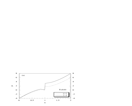
FIG. 2.: The chemical potential in the Roth’s method is reported as a function of the filling for $T=0.01$ and various values of U.

V COMPARISON WITH MONTE CARLO DATA

A well developed approach to the study of high correlated electron systems is based on the use of numerical techniques. There is now a considerable amount of numerical data on finite-dimension lattices; these results offer a precious guide and to them in any case all analytical formulations must refer. In this Section we shall present some local quantities, computed in the two-pole approximation. In particular, we consider the Roth’s method and the COM and compare the results with the numerical data by quantum Monte Carlo. In Fig. 3 the chemical potential is given as a function of the filling for $U=4$ and $T=0$.

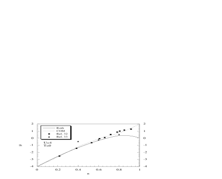
FIG. 3.: The chemical potential is given versus the filling $n$ for $T=0^{\circ}K$ and $U=4$. The solid and dotted lines represent the results in the Roth’s method and in the COM, respectively. The squares and the triangles refer to qMC data and have been taken from Refs. 32 and 33.

The solid line is the result of the Roth procedure; the dotted line is the result of COM. The theoretical data are compared with the numerical data by qMC, taken from Refs. 32 and 33.

FIG. 4.: The double occupancy as a function of n. The notation is the same as in Fig. 3. The qMC data are from Ref. 34.

We see that in the region $0.7<n<1$ the Roth results deviate from the behavior predicted by qMC, because of the unphysical downward deviation of the chemical potential.

The double occupancy $D=\langle n_{\uparrow}n_{\downarrow}\rangle$ and the energy per site $E_{s}=8t\langle c^{\alpha}(i)c^{\dagger}(i)\rangle+UD$ are reported as functions of n in Figs. 4 and 5, respectively. The Roth’s and COM’s results are compared with qMC data, taken from Ref. 34. The parameters have been fixed as $U=1,2,4$ and $T=1/6$.

FIG. 5.: The energy per site as a function of $n$. The notation is the same as in Fig. 3. The qMC data are from Ref. 34.

The results reported in the previous figures show a remarkable difference between the two formulations. In the two-pole approximation the method of the equation of motion [19-21] and the COM are equivalent, but they differ by the self-consistent procedure used to calculate the parameter p. The fact that the symmetry properties are not satisfied in the Roth’s scheme leads to the consequence that many properties are not conveniently calculated.

VI MOTT-HUBBARD TRANSITION.

Whether there exists a Mott-Hubbard transition, in the sense that at half filling there is a critical value of the Coulomb potential $U_{c}$ which separates the metallic phase from the insulating phase, is another problem still not fully understood in the context of the Hubbard model. In the case of one- dimensional system it is known that $U_{c}$ vanishes [35]; in higher dimensions there are no rigorous results. It is well known that Hubbard I approximation, defined by Eqs. (3.2)-(3.3), does not predict a metal-insulator transition: a gap in the density of states is present for any value of $U\neq 0$. This result led Hubbard to improve its approximation [36]. In this Section we shall consider the problem of the Mott-Hubbard transition at the light of the formulations discussed above.

In the case of half filling we have for the energy spectra the expressions

$$E_{1}({\rm\bf k})=R({\rm\bf k})+Q({\rm\bf k})\qquad E_{2}({\rm\bf k})=R({\rm\bf k})-Q({\rm\bf k})$$ (47)

with

$$R({\rm\bf k})=-8tp\alpha({\rm\bf k})\qquad Q({\rm\bf k})={1\over 2}\sqrt{U^{2}+[8t(2p-1)\alpha({\rm\bf k})]^{2}}$$ (48)

It is possible to show that in the Roth scheme for $n=1$ the minimum of $E_{1}({\rm\bf k})$ and the maximum of $E_{2}({\rm\bf k})$ are situated at ${\rm\bf k}=(\pi/2,\pi/2)$, so that

$$\Delta E=(E_{1})_{\min}-(E_{2})_{\max}=U$$ (49)

As in Hubbard I approximation, absence of a metal-insulator transition is found in the Roth’s method. In COM the minimum of $E_{1}({\rm\bf k})$ is situated at ${\rm\bf k}=(0,0)$, while the maximum of $E_{2}({\rm\bf k})$ is situated at ${\rm\bf k}=(\pi,\pi)$, so that

$$\Delta E=(E_{1})_{\min}-(E_{2})_{\max}=-16tp+\sqrt{U^{2}+[8t(2p-1)]^{2}}$$ (50)

The critical value of U which marks the Mott-Hubbard transition is then given by the self-consistent equation

$$U_{c}=8t\sqrt{4p-1}$$ (51)

This equation has been studied in Ref. 37. It has been found that $U_{c}$ slightly changes with temperature. At $T=0^{\circ}K$, $U_{c}=1.68W$, where $W$ is the bandwidth.

VII CONCLUSIONS

We have taken into considerations various methods [1, 13-31] that have been proposed to study systems with strong electronic correlations. At the lowest order all these methods coincide, in the sense that the spectral function of the single-particle Green’s function is approximated by a two-pole expansion, and finite life-times effects are neglected. Moreover, the analytic expression for the spectral function is the same in all considered methods and is expressed in terms of three self- consistent parameters. While two parameters, the chemical potential $\mu$ and the static correlation function $\Delta\equiv\langle\xi^{\alpha}(i)\xi^{\dagger}(i)\rangle-\langle\eta^{\alpha}(i)\eta^{\dagger}(i)\rangle$ are controlled by the dynamics through the self-consistent equations (3.1) and (3.4), there is some freedom in the determination of the parameter $p$, defined by Eq. (2.21), and different choices have been proposed. Most of the works follow the procedure suggested by Roth [20], where use has been made of the equation of motion in the linearized form (2.11). However, we have shown that this choice violates the Pauli principle and the particle-hole symmetry. As a consequence, the solution provides many unpleasant results: the compressibility becomes negative in the region of filling $0.7<n<1$, there is absence of a Mott-Hubbard transition, the calculated values for some local quantities strongly disagree with the numerical data by qMC. We have shown that all these undesirable features disappear when the Pauli principle is recovered.

The matrix energy must be calculated in a self-consistent way, but there is some freedom in choosing the procedure. We can take advantage of this freedom to fix the self-consistent procedure in such a way that the Hilbert space has the right properties of symmetry. In the framework of two-pole approximation the unique way to realize this is to require that the Pauli amplitude (3.8) vanishes.

A EQUAL-TIME CORRELATION FUNCTIONS

By standard methods equal-time correlation functions can be calculated by means of the retarded Green’s function. Indeed, one has

$$C_{\Psi\Psi}({\rm\bf R}_{i},{\rm\bf R}_{j})\equiv\langle\Psi({\rm\bf R}_{i})\Psi^{\dagger}({\rm\bf R}_{j})\rangle={a^{2}\over(2\pi)^{2}}\int d^{2}kd\omega[1-f_{F}(\omega)]\left(-{1\over\pi}\right)Im[S_{\Psi\Psi}({\rm\bf k},\omega)]$$ (A.1)

where $S_{\Psi\Psi}({\rm\bf k},\omega)$ is the Fourier transform of the Green’s function. $f_{F}(\omega)$ is the Fermi distribution function and $\Omega_{B}$ is the first Brillouin zone. By means of Eq. (2.15) we have

$$C_{\Psi\Psi}({\rm\bf R}_{i},{\rm\bf R}_{j})={\Omega\over 2(2\pi)^{2}}\sum^{2}_{i=1}\int_{\Omega_{B}}d^{2}ke^{i{{\rm\bf k}}\cdot({\rm\bf R}_{i}-{\rm\bf R}_{j})}[1+T_{i}({\rm\bf k})]\sigma^{(i)}_{\Psi\Psi}({\rm\bf k})$$ (A.2)

where

$$T_{i}({\rm\bf k})=\tanh\left({E_{i}({\rm\bf k})\over 2k_{B}T}\right)$$ (A.3)

Let us use the notation

$$C_{\Psi\Psi}=C_{\Psi\Psi}({\rm\bf R}_{i},{\rm\bf R}_{i})\qquad C^{\alpha}_{\Psi\Psi}=C_{\Psi\Psi}({\rm\bf R}_{i},{\rm\bf R}_{i\pm a})$$ (A.4)

By using the definition (2.23) for the spectral function we easily obtain the following expressions

$$C_{\xi\xi} = \langle\xi(i)\xi^{\dagger}(i)\rangle={I_{1}\over 2}\left[1+G_{0}-UF_{0}+{1-n\over{I_{1}I_{2}}}B_{0}\right]$$ (A.5)

$$C_{\xi\eta} = \langle\xi(i)\eta^{\dagger}(i)\rangle=B_{0}$$ (A.6)

$$C_{\eta\eta} = {I_{2}\over 2}\left[1+G_{0}+UF_{0}-{1-n\over I_{1}I_{2}}B_{0}\right]$$ (A.7)

$$C^{\alpha}_{\xi\xi} = \langle\xi^{\alpha}(i)\xi^{\dagger}(i)\rangle={I_{1}\over 2}\left[G_{1}-UF_{1}+{1-n\over{I_{1}I_{2}}}B_{1}\right]$$ (A.8)

$$C^{\alpha}_{\xi\eta} = \langle\xi^{\alpha}(i)\eta^{\dagger}(i)\rangle=B_{1}$$ (A.9)

$$C_{\eta\eta} = {I_{2}\over 2}\left[G_{1}+UF_{1}-{1-n\over I_{1}I_{2}}B_{1}\right]$$ (A.10)

where we have defined

$$F_{n} = {\Omega\over 2(2\pi)^{2}}\int_{\Omega_{B}}d^{2}k{[\alpha({\rm\bf k})]^{n}\over 2Q({\rm\bf k})}[T_{1}({\rm\bf k})-T_{2}({\rm\bf k})]$$ (A.11)

$$G_{n} = {\Omega\over 2(2\pi)^{2}}\int_{\Omega_{B}}d^{2}k[\alpha({\rm\bf k})]^{n}[T_{1}({\rm\bf k})+T_{2}({\rm\bf k})]$$ (A.12)

$$B_{n} = {\Omega\over 2(2\pi)^{2}}\int_{\Omega_{B}}d^{2}k[\alpha({\rm\bf k})]^{n}{m({\rm\bf k})\over 2Q({\rm\bf k})}[T_{1}({\rm\bf k})-T_{2}({\rm\bf k})]$$ (A.13)

In the text, in order to compare different methods, we are also using the following correlation functions

$$\begin{array}[]{ll}C_{cc}=\langle c(i)c^{\dagger}(i)\rangle=C_{\xi\xi}+2C_{\xi\eta}+C_{\eta\eta}&\quad C_{c\eta}=\langle c(i)\eta^{\dagger}(i)\rangle=C_{\xi\eta}+C_{\eta\eta}\\ C^{\alpha}_{cc}=\langle c^{\alpha}(i)c^{\dagger}(i)\rangle=C^{\alpha}_{\xi\xi}+2C^{\alpha}_{\xi\eta}+C_{\eta\eta}&\quad C^{\alpha}_{c\eta}=\langle c^{\alpha}(i)\eta^{\dagger}(i)\rangle=C^{\alpha}_{\xi\eta}+C^{\alpha}_{\eta\eta}\\ \end{array}$$ (A.14)

B CONSERVATION OF THE FIRST FOUR SPECTRAL MOMENTA

Let us show that the first four momenta of the electron spectral density satisfy the exact relations given by Eq. (2.26). By straightforward calculations we can see that:

$$M^{(0)}({\rm\bf k}) = F.T.\langle\left\{c(i),c^{\dagger}(j)\right\}\rangle=1$$ (B.1)

$$M^{(1)}({\rm\bf k}) = F.T.\langle\left\{\left(i{\partial\over\partial t}\right)c(i),c^{\dagger}(j)\right\}\rangle=-\mu+{n\over 2}U-4t\alpha({\rm\bf k})$$ (B.2)

$$M^{(2)}({\rm\bf k}) = F.T.\langle\left\{\left(i{\partial\over\partial t}\right)^{2}c(i),c^{\dagger}(j)\right\}\rangle=-\mu M^{(1)}({\rm\bf k})+U\left[m({\rm\bf k})-(\mu-U){n\over 2}-4t(\Delta+\alpha({\rm\bf k})p)\right]$$ (B.4)

$$-4tF.T.\sum_{l}\alpha_{il}\langle\left\{\left(i{\partial\over\partial t}\right)c(l),c^{\dagger}(j)\right\}\rangle=$$

$$= \mu^{2}-\mu nU+{n\over 2}U^{2}+16t^{2}\alpha^{2}({\rm\bf k})+8t\mu\alpha({\rm\bf k})-8t{n\over 2}U\alpha({\rm\bf k})$$ (B.5)

$$M^{(3)}({\rm\bf k}) = F.T.\langle\left\{\left(i{\partial\over\partial t}\right)^{2}c(i),\left(-i{\partial\over\partial t^{\prime}}\right)c^{\dagger}(j)\right\}\rangle$$ (B.6)

$$= -\mu M^{(2)}({\rm\bf k})+F.T.\langle\left\{-\mu\left(i{\partial\over\partial t}\right)c(i)+U\left(i{\partial\over\partial t}\right)\eta(i)-4t\sum_{l}\alpha_{il}\left(i{\partial\over\partial t}\right)c(l),U\eta^{\dagger}(j)-4t\sum_{m}\alpha_{mj}c^{\dagger}(m)\right\}\rangle$$ (B.7)

$$= \left[-4t\alpha({\rm\bf k})-\mu\right]^{3}+3{n\over 2}U\left[-4t\alpha({\rm\bf k})-\mu\right]^{2}+{n\over 2}U^{3}-3{n\over 2}\mu U^{2}-8t{n\over 2}U^{2}\alpha({\rm\bf k})-4t\Delta U^{2}-4tpU^{2}\alpha(k)$$ (B.8)

On the other hand, from Eqs. 2.23 - 2.25 we have

$$M^{(0)}({\rm\bf k}) = \sum^{2}_{i=1}\left[\sigma^{(i)}_{\xi\xi}({\rm\bf k})+2\sigma^{(i)}_{\xi\eta}({\rm\bf k})+\sigma^{(i)}_{\eta\eta}({\rm\bf k})\right]=1$$ (B.9)

$$M^{(1)}({\rm\bf k}) = \sum^{2}_{i=1}\left[\sigma^{(i)}_{\xi\xi}({\rm\bf k})+2\sigma^{(i)}_{\xi\eta}({\rm\bf k})+\sigma^{(i)}_{\eta\eta}({\rm\bf k})\right]E_{i}({\rm\bf k})$$ (B.10)

$$= R({\rm\bf k})M^{(0)}({\rm\bf k})+Q({\rm\bf k})\left[{I_{1}-I_{2}\over 2}{g({\rm\bf k})\over Q({\rm\bf k})}+2{m({\rm\bf k})\over Q({\rm\bf k})}\right]=-\mu+{n\over 2}U-4t\alpha({\rm\bf k})$$ (B.11)

From Eq. (B.6) follows the identity

$${I_{1}-I_{2}\over 2}{g({\rm\bf k})\over Q({\rm\bf k})}+2{m({\rm\bf k})\over Q({\rm\bf k})}=-{R({\rm\bf k})\over Q({\rm\bf k})}+{M^{(1)}({\rm\bf k})\over Q({\rm\bf k})}$$ (B.12)

that leads to

$$M^{(2)}({\rm\bf k}) = \sum^{2}_{i=1}\left[\sigma^{(i)}_{\xi\xi}({\rm\bf k})+2\sigma^{(i)}_{\xi\eta}({\rm\bf k})+\sigma^{(i)}_{\eta\eta}({\rm\bf k})\right]E^{2}_{i}({\rm\bf k})$$ (B.13)

$$= \left[R^{2}({\rm\bf k})+Q^{2}({\rm\bf k})\right]M^{(0)}({\rm\bf k})+2R({\rm\bf k})Q({\rm\bf k})\left[-{R({\rm\bf k})\over Q({\rm\bf k})}+{M^{(1)}({\rm\bf k})\over Q({\rm\bf k})}\right]$$ (B.14)

$$= \mu^{2}-\mu nU+{n\over 2}U^{2}+16t^{2}\alpha^{2}({\rm\bf k})+8t\mu\alpha({\rm\bf k})-8t{n\over 2}U\alpha({\rm\bf k})$$ (B.15)

$$M^{(3)}({\rm\bf k}) = \sum^{2}_{i=1}\left[\sigma^{(i)}_{\xi\xi}({\rm\bf k})+2\sigma^{(i)}_{\xi\eta}({\rm\bf k})+\sigma^{(i)}_{\eta\eta}({\rm\bf k})\right]E^{3}_{i}({\rm\bf k})$$ (B.16)

$$= \left[R^{3}({\rm\bf k})+3R({\rm\bf k})Q^{2}({\rm\bf k})\right]M^{(0)}({\rm\bf k})+\left[Q^{3}({\rm\bf k})+3R^{2}({\rm\bf k})Q({\rm\bf k})\right]\left[-{R({\rm\bf k})\over Q({\rm\bf k})}+{M^{(1)}({\rm\bf k})\over Q({\rm\bf k})}\right]$$ (B.17)

$$= 2R({\rm\bf k})M^{(2)}({\rm\bf k})+\left[Q^{2}({\rm\bf k})-R^{2}({\rm\bf k})\right]M^{(1)}({\rm\bf k})$$ (B.18)

$$= \left[-4t\alpha({\rm\bf k})-\mu\right]^{3}+3{n\over 2}U\left[-4t\alpha({\rm\bf k})-\mu\right]^{2}+{n\over 2}U^{3}-3{n\over 2}\mu U^{2}-8t{n\over 2}U^{2}\alpha({\rm\bf k})-4t\Delta U^{2}-4tpU^{2}\alpha(k)$$ (B.19)

Then, there is a complete equivalence among all considered theoretical approaches, when two-pole approximation is used.

REFERENCES

- [1] J. Hubbard, Proc. Roy. Soc. London A 276, 238 (1963).
- [2] P.W. Anderson, Science 235, 1196 (1987).
- [3] S.E. Barnes, J. Phys. F 6, 1375 (1976); ibid 7, 2637 (1977).
- [4] P. Coleman, Phys. Rev. B 29 , 3035 (1984).
- [5] G. Kotliar and A.E. Ruckenstein, Phys. Rev. Lett. 57, 1362 (1986).
- [6] Y. Kuramoto, Z. Phys. B 53, 37 (1983).
- [7] N. Grewe, Z. Phys. B 53, 271 (1983).
- [8] Th. Pruschke, Z. Phys. B 81, 319 (1990).
- [9] W. Metzner and D. Vollhardt, Phys. Rev. Lett. 62, 324 (1989).
- [10] A. Georges and G. Kotliar, Phys. Rev. B 45, 6479 (1992).
- [11] A. Georges and W. Krauth, Phys. Rev. B 48, 7167 (1993).
- [12] M.J. Rosenberg, G. Kotliar and X.Y. Zhang, Phys. Rev. B 49, 10191 (1994).
- [13] K.W. Becker, W. Brenig and P. Fulde, Z. Phys. B 81, 165 (1990).
- [14] H. Mori, Progr. Theor. Phys. 33, 423 (1965); ibid 34, 399 (1965).
- [15] A.J. Fedro, Yu Zhou, T.C. Leung, B.N. Harmon and S.K. Sinha, Phys. Rev. B 46, 14785 (1992).
- [16] P. Fulde, Electron Correlations in Molecules and Solids (Springer-Verlag, Berlin-Heidelberg, 1993).
- [17] N.M. Plakida, V.Yu. Yushankhai and I.V. Stasyuk, Physica C 162-164, 787 (1989).
- [18] B. Mehlig, H. Eskes, R. Hayn and M.B.J. Meinders, Phys. Rev. B 52, 2463 (1995).
- [19] D.J. Rowe, Rev. Mod. Phys. 40, 153 (1968).
- [20] L.M. Roth, Phys. Rev. 184, 451 (1969).
- [21] J. Beenen and D.M. Edwards, Phys. Rev. B 52, 13636 (1995).
- [22] O.K. Kalashnikov and E.S. Fradkin, Phys. Stat. Sol. (b) 59, 9 (1973).
- [23] W. Nolting, Z. Phys. 255, 25 (1972); G. Geipel and W. Nolting, Phys. Rev. B 38, 2608 (1988); W. Nolting and W. Borgel, Phys. Rev. B 39, 6962 (1989).
- [24] A. Lonke, J. Math. Phys. 12, 2422 (1971).
- [25] I. Ishihara, H. Matsumoto, S. Odashima, M. Tachiki and F. Mancini, Phys. Rev. B 49, 1350 (1994).
- [26] F. Mancini, S. Marra and H. Matsumoto, Physica C 244, 49 (1995).
- [27] F. Mancini, S. Marra and H. Matsumoto, Physica C 250, 184 (1995).
- [28] F. Mancini, S. Marra and H. Matsumoto, Physica C 252, 361 (1995).
- [29] F. Mancini, S. Marra, D. Villani and H. Matsumoto, Physics Letters A 210, 429 (1996).
- [30] H. Matsumoto, T. Saikawa and F. Mancini, Phys. Rev. B 54, 14445 (1996).
- [31] H. Matsumoto and F. Mancini, Phys. Rev. B 55, 2095 (1997).
- [32] N. Furukawa and M. Imada, J. Phys. Soc. Jpn. 61, 3331 (1992); N. Furukawa and M. Imada, Physica B 186-188, 931 (1993).
- [33] E. Dagotto, A. Moreo, F. Ortolani, D. Poilblanc and J. Riera, Phys. Rev. B 45, 10741 (1992).
- [34] A. Moreo, D.J. Scalapino, R.L. Sugar, S.R. White and N.E. Bickers, Phys. Rev. B 41, 2313 (1990).
- [35] E.H. Lieb and F.Y. Wu, Phys. Rev. Lett. 20, 1445 (1968).
- [36] J. Hubbard, Proc. Roy. Soc. London A 281, 401 (1964).
- [37] F. Mancini, M. Marinaro and H. Matsumoto, Int. Journ. Mod. Phys. B 10, 1717 (1996).