Determination of the universality class of Gadolinium

Abstract

We resolve a longstanding puzzle for the static and dynamic critical behavior of Gadolinium by a combined theoretical and experimental investigation. It is shown that the spin dynamics of a three dimensional ferromagnet with hcp lattice structure and a spin-spin interaction given by both exchange and dipole-dipole interaction belongs to a new dynamic universality class, model J^∗. Comparing results from mode coupling theory with results from three different hyperfine interaction probes we find quantitative agreement. The crossover scenario for the wavevector dependence of the hyperfine relaxation rate is determined by a subtle interplay between three length scales: the correlation length, the dipolar and the uniaxial wave vector.

The spin dynamics of simple ferromagnets in the vicinity of their Curie point $T_{c}$ are archetypical examples of dynamic critical phenomena near second-order phase transitions. Much experimental and theoretical effort has been put into identifying the dynamic universality classes and assigning them to magnetic substances. Nevertheless, experimental observations on gadolinium [1, 2, 3, 4, 5, 6, 7] remained a puzzle up to now. Because of its large localized magnetic moment, and the fact that it is an S-state ion, Gd should have a very small magnetocrystalline anisotropy and therefore be much better a model system for an isotropic Heisenberg magnet than either Fe, Ni or EuO. As a consequence it should belong to the model J dynamic universality class in the classification scheme of Ref. [8]. The measured static and especially dynamic critical exponents are, however, not at all compatible with model J. The objective of this paper is to resolve this longstanding seemingly contradictory situation by a combined theoretical and experimental study.

Early experimental observations [9] clearly demonstrate that Gd has an easy axis which coincides with the hexagonal axis of its hcp lattice. The origin of such an easy axis cannot be understood from the magnetocrystalline anisotropy. But, based on a mean field theory [10] it has been argued that a combined effect of the lattice structure and dipolar interaction favors the c-axis as the easy direction. This view is supported by measurements [7] of the c-axis and basal-plane susceptibility on a single crystal of Gd. It is found that the basal-plane susceptibility crosses over from a singular behavior to a constant at a characteristic temperature scale which can be accounted for by dipolar effects. The analysis of the static critical behavior [7] is, however, complicated by the fact that all experiments are done in the non-asymptotic regime where superposed crossover lead to complex temperature dependences. This may not be easily interpreted in terms of one or the other universality class. This is even more so, as the static critical exponents for the various universality classes are of comparable magnitude.

A surprising and yet unexplained observation was made by a measurement of the critical dynamics using hyperfine methods [1, 2, 3]. The critical exponent $w$ for the autocorrelation time $\tau_{c}$, which should scale as $\tau_{c}\propto(T-T_{c})^{-w}$ in the asymptotic regime, was found to be $w\approx 0.5$. The observed value is not consistent with either Heisenberg or Ising models, but considerably lower.

The purpose of this letter is twofold. First we give a theoretical description for a spin system with both exchange and dipolar interaction on a hcp lattice using mode coupling theory. Next we calculate the relaxation rates observed in various hyperfine interaction measurements, where we account for the details of the coupling tensor in each of these methods. We also report on measurements of the muon spin relaxation ($\mu$SR) rate in high purity single crystal samples of Gd. A comparison of the theoretical predictions with these and earlier [4, 6] $\mu$SR measurements as well as perturbed angular correlation (PAC) and Moessbauer data [1, 2, 3] gives a coherent picture of the dynamic and static critical behavior of Gd and resolves the puzzling situation described above.

We consider a system with $N$ identical spins fixed on the sites of a three dimensional lattice. Taking into account magnetocrystalline anisotropy as well as dipolar interaction it is described by the Hamiltonian

$$H=-\!\sum_{i\neq j}\left[J_{ij}^{\perp}\left(S^{x}_{i}\!S^{x}_{j}\!+\!S^{y}_{i}\!S^{y}_{j}\right)\!+\!J_{ij}^{\parallel}S^{z}_{i}\!S^{z}_{j}\!+\!D_{ij}^{\alpha\beta}S_{i}^{\alpha}\!S_{j}^{\beta}\right].$$ (1)

The magnitude of the magnetocrystalline anisotropy of the system is characterized by $\Delta=J^{\parallel}/J^{\perp}$. The dipolar interaction is characterized by the tensor

$$D_{ij}^{\alpha\beta}=-\frac{(g_{L}\mu_{B})^{2}}{2}\left(\frac{\delta_{\alpha\beta}}{|{\bf x}_{ij}|^{3}}-\frac{3x_{ij}^{\alpha}x_{ij}^{\beta}}{|{\bf x}_{ij}|^{5}}\right),$$ (2)

with ${\bf x}_{ij}={\bf x}_{i}-{\bf x}_{j}$, $g_{L}$ is the Landé factor, and $\mu_{B}$ the Bohr magneton. Dipolar lattice sums, $D_{\bf q}^{\alpha\beta}=\sum_{i\neq j}D_{ij}^{\alpha\beta}e^{i{\bf q}\cdot{\bf x}_{i}}$, can be evaluated by using Ewald’s method. For infinite three–dimensional cubic lattices the results may be found in Ref. [11, 12]. For Bravais lattices with a hexagonal-closed packed (hcp) structure the dipolar tensor to leading order in ${\bf q}$ becomes [10]

$$D_{\bf q}^{\alpha\beta}=\frac{(g_{L}\mu_{B})^{2}}{2v_{a}}\left[\beta_{4}^{\alpha}\delta_{\alpha\beta}-4\pi\frac{q_{\alpha}q_{\beta}}{q^{2}}+{\cal O}(q^{2})\right],$$ (3)

where $v_{a}$ is the volume of the primitive unit cell with lattice constant $a$, and the parameters are $\beta_{4}^{x}=4.12$ and $\beta_{4}^{z}=4.32$. Upon expanding the Fourier transform of the exchange interaction $J_{\bf q}^{\alpha}={\sum_{i}}^{\prime}J_{i0}^{\alpha}e^{i{\bf q}\cdot{\bf x}_{i}}\approx J_{0}^{\alpha}-Jq^{2}a^{2}+{\cal O}(q^{4})$, and keeping only those terms which are relevant in the spirit of the renormalization group theory, one finds

$$H=J\sum_{\bf q}\Biggl{[}\biggl{(}m^{\alpha}-\Delta_{0}^{\alpha}+q^{2}a^{2}\biggr{)}\delta_{\alpha\beta}+g\frac{q_{\alpha}q_{\beta}}{q^{2}}\Biggr{]}S^{\alpha}_{-\bf q}S^{\beta}_{\bf q}.$$ (4)

There are two sources of uniaxial anisotropy in the Hamiltonian, Eq. 4, magnetocrystalline anisotropy, $\Delta_{0}^{\alpha}=J_{0}^{\alpha}/J$, and dipolar interaction, $m^{\alpha}=(g_{L}\mu_{B})^{2}\beta_{4}^{\alpha}/2Jv_{a}$. In addition, the dipolar interaction introduces an anisotropy of the spin-fluctuations with respect to the wave vector ${\bf q}$ which is reflected by the term proportional to $q_{\alpha}q_{\beta}/q^{2}$. The magnitude $g$ of this anisotropy is given by $g=4\pi(g_{L}\mu_{B})^{2}/2Jv_{a}$. We define a dimensionless quantity $m=(g_{L}\mu_{B})^{2}(\beta_{4}^{\parallel}-\beta_{4}^{\perp})/2Jv_{a}$ proportional to the ratio of the anisotropy energy and the exchange energy. Putting in values for Gd the ratio of the dipolar contribution to the term $q_{\alpha}q_{\beta}/q^{2}$ and to the uniaxial anisotropy is $\sqrt{g/m}=7.8738$. In the following we will show that all available data for Gd can be explained by assuming that the uniaxial anisotropy is solely due to the dipolar interaction. Therefore, we will assume $\Delta=0$ in the following discussion.

Now we turn to an analysis of the static critical behavior. In Ornstein-Zernike approximation the static susceptibility reads

$$\chi^{-1}_{\alpha\beta}({\bf q})=J\left[(r_{\alpha}+q^{2})\,\delta_{\alpha\beta}+q_{D}^{2}\,\frac{q_{\alpha}q_{\beta}}{q^{2}}\right],$$ (5)

where $r_{z}=r=\xi^{-2}$, $r_{x,y}=\xi^{-2}+q_{A}^{2}$ and we have measured all length scales in units of the lattice constant $a$. The analysis of the critical behavior resulting from the Hamiltonian, Eq. 4, is complicated by the fact that besides the correlation length $\xi=\xi_{0}(T/T_{c}-1)^{-\nu}$ there are two anisotropy length scales $q_{A}^{-1}=a/\sqrt{m}$ and $q_{D}^{-1}=a/\sqrt{g}$, both resulting from the dipolar interaction. The eigenvalues of the inverse susceptibility matrix are given by $\lambda_{1}({\bf q})=q^{2}+\xi^{-2}+q_{A}^{2}$ and $\lambda_{2,3}({\bf q})=q^{2}+\xi^{-2}+\left[q_{D}^{2}+q_{A}^{2}\pm W\right]/2$ where $W=[(q_{D}^{2}+q_{A}^{2})^{2}-4q_{D}^{2}q_{A}^{2}q_{z}^{2}/q^{2}]^{1/2}$; the eigenvectors ${\bf e}_{i}({\bf q})$ are given in a forthcoming publication [13]. It is interesting to note that due to the combined effect of the dipolar interaction and the uniaxial anisotropy of the lattice the eigenvalues of the susceptibility matrix remain finite in the limit $q\rightarrow 0$ and upon approaching the critical temperature. Only if the angle $\vartheta$ between the easy axis ($z$-axis) of magnetization and the wave vector is $\vartheta=90^{o}$ the third eigenvalue becomes critical. Due to the anisotropy terms in the Hamiltonian there are two crossover as a function of the reduced temperature and wave vector. To a good approximation these can be incorporated in an effective exponent of the correlation length $\xi$ [14].

Mode coupling theory is a theoretical method which has been shown to give highly accurate results for the critical dynamics of cubic ferromagnets [12]. Here we generalize this method to non-cubic magnets. Starting from the equations of motion for the components $s^{\alpha}_{\bf q}$ of the spin ${\bf S}_{\bf q}$ in the eigenvector basis, $s^{\alpha}_{\bf q}=\sum_{i}S^{i}_{\bf q}e_{\alpha i}({\bf q})$, one can derive the following set of coupled integral equations [13] for the half-sided Fourier transform, $\Phi_{\alpha}({\bf q},\omega)=i\chi_{\alpha}({\bf q})/[\omega+i\Gamma_{\alpha}({\bf q},\omega)]$, of the Kubo relaxation function $\Phi_{\alpha\beta}({\bf q},t)$,

$$\Gamma_{\alpha}({\bf q},\omega) = \frac{4k_{B}TJ^{2}}{\chi_{\alpha}({\bf q})}\int_{{\bf k},\omega^{\prime}}\sum_{\beta\gamma}K^{\beta\gamma}_{\alpha}({\bf k},{\bf q})$$ (6)

$$\times \Phi_{\beta}({\bf k},\omega)\Phi_{\gamma}({\bf q}\!-\!{\bf k},\omega\!-\!\omega^{\prime}),$$ (7)

where $\int{{\bf k},\omega}=\int(d^{3}k/(2\pi)^{3})\int(d\omega/2\pi)$. The vertex functions $K^{\beta\gamma}_{\alpha}({\bf k},{\bf q})$ for the decay of the mode $\alpha$ into the modes $\beta$ and $\gamma$ are given by [13]

$$K^{\beta\beta}_{\alpha}({\bf k},{\bf q}) = T^{\beta\beta}_{\alpha}({\bf k},{\bf q})U_{\alpha\beta}^{\beta}({\bf k},{\bf q})\left[\lambda_{\beta}({\bf k})-\lambda_{\beta}({\bf q}-{\bf k})\right],$$ (8)

$$K^{\beta\gamma}_{\alpha}({\bf k},{\bf q}) = T^{\beta\gamma}_{\alpha}({\bf k},{\bf q})\,T^{\beta\gamma}_{\alpha}({\bf k},{\bf q}),\quad\beta\not=\gamma,$$ (9)

with $U_{\alpha\beta}^{\gamma}({\bf k},{\bf q})=\sum_{ijk}\varepsilon_{ijk}\,e_{\alpha i}({\bf k})\,e_{\beta j}({\bf q})\,e_{\gamma k}({\bf q}-{\bf k})$, where $\varepsilon_{ijk}$ is the Levi-Cevita symbol, and $T^{ii}_{\alpha}({\bf k},{\bf q})=\lambda_{i}({\bf k})U_{i\alpha}^{i}({\bf k},{\bf q})$, $T^{ij}_{\alpha}({\bf k},{\bf q})=\left[\lambda_{i}({\bf k})-\lambda_{j}({\bf q}\!-\!{\bf k})\right]U_{i\alpha}^{j}({\bf k},{\bf q})$ for $i<j$ and $T^{ij}_{\alpha}({\bf k},{\bf q})=0$ for $i>j$. In the limits $q_{D}\rightarrow 0$ or $q_{A}\rightarrow 0$ these equations reduce either to the uniaxial or to the isotropic dipolar ferromagnet [12, 15]

We have solved the above mode coupling equations in the Lorentzian approximation for the lineshape [13]. It is found that the mode coupling equations obey a generalized dynamic scaling law where the linewidth depend on three scaling variables, $x_{1}=1/q\xi$, $x_{2}=q_{D}/q$ and $x_{3}=q_{A}/q$, and the angle $\vartheta$ between the direction of the wave vector and the $z$-axis. The explicit functional form is too complicated to be presented in this letter and we refer the reader to a forthcoming publication [13]. But, note that it is implicitly contained in the damping rates for the hyperfine interaction probes discussed below.

Now we compare the above theoretical results with experimental data obtained from hyperfine interaction experiments. We have performed zero field $\mu$SR experiments on Gd [16]. Spin polarized muons were implanted in order to measure the distribution and the dynamics of the internal magnetic field at the muon site via the temporal loss of the initial spin polarization. The experiments were performed at the $\mu$SR facility of the Paul Scherrer Institute using a high momentum muon beam. The sample was a spherical Gd single crystal with diameter $2.5$ cm. The temperature could be stabilized to at least $\pm 0.05K$. We could describe the temporal loss of the initial muon spin polarization by an exponential decay function $P(t)=\exp\left(-\lambda_{z}t\right)$. Taking into account anisotropic dipolar fields as well as the isotropic Fermi contact field to the local field at the muon site the muon damping rate can be written as [17, 18, 13]

$$\lambda_{\hat{z}}=\frac{\pi{\cal D}}{V^{2}}\int_{{\bf q}}\sum_{{\hat{\beta}}{\hat{\gamma}}}\left[G^{{\hat{x}}{\hat{\beta}}}_{\bf q}G^{{\hat{x}}{\hat{\gamma}}}_{-{\bf q}}+G^{{\hat{y}}{\hat{\beta}}}_{\bf q}G^{{\hat{y}}{\hat{\gamma}}}_{-{\bf q}}\right]\Phi^{{\hat{\beta}}{\hat{\gamma}}}({\bf q},0),$$ (10)

where the hatted variables indicate that the corresponding quantities have to be evaluated in the muon reference frame, i.e. the ${\hat{z}}$-axis coincides with the initial polarization of the muon beam. Here we have defined ${\cal D}=\gamma_{\mu}^{2}(\mu_{0}/4\pi)^{2}(g_{L}\mu_{B})^{2}$. The coupling of the muon spin and the spins of the magnet is described in terms of the coupling matrix $G^{{\hat{x}}{\hat{\beta}}}_{\bf q}$, which reflects the particular symmetry of the lattice sites occupied by the muons. Since the most dominant contribution to the damping rate comes from wave vectors close to the Brillouin zone center, the form of the coupling tensor $G^{{\hat{x}}{\hat{\beta}}}_{\bf q}$ at small values of ${\bf q}$ will be important. In the limit ${\bf q}\to 0$ [18, 13] one finds $G^{\alpha\beta}_{{\bf q}\to 0}=-4\pi\left[{q_{\alpha}q_{\beta}/q^{2}}-p_{\alpha}\right],$ with $p_{\alpha}=d_{\alpha}+n_{\mu}H_{\mu}/4\pi$. With the Fermi contact field $B_{\rm FC}=-6.98$ kG at $T=0$ K [19], one gets $n_{\mu}H_{\mu}/4\pi=-0.278$ [18], and consequently for octahedral sites $p_{x}=p_{y}=0.0705$ and $p_{z}=0.0250$ [18], and for tetrahedral sites $p_{x}=p_{y}=0.0338$ and $p_{z}=0.0984$ [13]. The muon relaxation rate $\lambda_{z}$ depends on the material parameters $q_{A}\xi_{0}$ and $q_{D}\xi_{0}$. Since we assume that both anisotropies result from the dipolar interaction the ratio $q_{D}/q_{A}=7.8738$ is known and the number of material parameters is reduced to one. In comparing our theory with $\mu$SR experiments at a polarization $\alpha=90^{o}$ we get the best fit to the data with $q_{D}\xi_{0}=0.13$ (see Fig. 1). This results in the following values for the uniaxial and dipolar wave vector, $q_{A}=0.0165/\xi_{0}$, $q_{D}=0.13/\xi_{0}$. The corresponding crossover temperatures are given by $T_{A}=T_{c}+0.43$ K and $T_{D}=T_{c}+16.54$ K suggesting the following crossover scenario. For $T\gg T_{D}$ we expect critical behavior dominated by the (isotropic) Heisenberg fixed point. The relaxation rate shows power law behavior $\lambda\propto t^{-w},$ with an exponent $w\approx 1$. For temperatures in the interval $T_{D}>T>T_{A}$ dipolar interaction becomes important. But, from the analysis of the uniaxial crossover [13] it turns out that the uniaxial crossovers in dynamics sets in at wave vectors much larger than expected from an analysis of the static quantities. Therefore, even for $T>T_{A}$ we expect to observe effects from dipolar interaction as well as uniaxial anisotropy. Finally, for $T<T_{A}$ the critical dynamics is determined by the uniaxial dipolar fixed point. Then the static susceptibilities do no longer diverge for $q\rightarrow 0$ and $T\rightarrow T_{c}$ except when the wave vector is perpendicular to the easy axis of magnetization. Since the relaxation rate $\lambda_{z}$ is given by an integral over the whole Brillouin zone, the relative weight of the critical axis along which the susceptibility diverges becomes vanishingly small. As a consequence the relaxation rate $\lambda_{z}$ no longer diverges for $T\rightarrow T_{c}$, i.e. $w\rightarrow 0$ (compare Fig. 1).

Fig. 1 shows a comparison between the theoretical and experimental results for an initial polarization inclined by an angle $\alpha=90^{o}$ with respect to the easy axis of magnetization. The solid line and the dashed line are the theoretical result for the muon relaxation rate if the muons penetrating the sample are located at tetrahedral and octahedral interstitial sites, respectively. The comparison between theory and experiment favors tetrahedral sites. This is confirmed by $\mu$SR experiments with the initial polarization along the easy axis of magnetization. The ratio $\lambda_{z}(90^{o})/\lambda_{z}(0^{o})$ for $T\rightarrow T_{c}$ becomes $1.2$ and $0.7$ for octahedral and tetrahedral sites, respectively [16]. The experiment is closer to the latter value strongly suggesting that muons occupy octahedral sites within the Gd lattice.

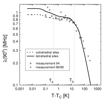
FIG. 1.: Experimental and theoretical results of the relaxation rate $\lambda$ for tetrahedral and octahedral muon sites with $\alpha=90^{o}$. Data taken from Ref. [6, 4] and measured at the $\mu$SR facility at the PSI in 1992 and 1994 (see inset) [16]

The coupling tensor in PAC and Moessbauer measurements reduces to a Fermi contact coupling. As a consequence the observed relaxation rate is a sum over the eigenmodes $\tau_{c}=(k_{B}T/3v_{a})\sum_{\alpha}\int_{\bf q}\chi_{\alpha}({\bf q})/\Gamma_{\alpha}({\bf q})$. Important information about the behavior of the auto-correlation time can be gained from a scaling analysis. An effective dynamical exponent $z_{\rm eff}$ may defined by $\tau_{c}\propto\left(T-T_{c}\right)^{-w_{\rm eff}}$ with $w_{\rm eff}=\nu_{\rm eff}(z_{\rm eff}-1)$, where we have neglected the Fisher exponent $\eta$. If dipolar interaction and uniaxial anisotropy were absent, one would expect $w\approx 1.0$. The dipolar interaction is known to be a relevant perturbation at the Heisenberg fixed point. It leads to asymptotic static critical exponents which are only slightly different from the corresponding Heisenberg values. But, since dipolar interaction implies a non-conserved order parameter the asymptotic dynamic exponent becomes $z_{\rm D}\approx 2$ resulting in a crossover from $w_{\rm I}\approx 1.0$ to $w_{\rm D}\approx 0.7$. Uniaxial interaction is also known to be a relevant perturbation with respect to the Heisenberg fixed point. Again, the static critical exponents are not changed very much, e.g. one finds the Ising (I) value $\nu_{\rm I}=0.63$, but the dynamic exponent becomes $z_{\rm I}\approx 4$ if the order parameter is conserved ($z_{\rm I}\approx 2$ otherwise). The corresponding exponent for the hyperfine relaxation rate would turn out to be $w_{\rm I}\approx 1.89$ and $w_{\rm I}\approx 0.63$ for conserved and non-conserved order parameter, respectively. According to these scaling arguments it is hard to think of any dynamic universality class which could lead to an effective exponent $w_{\rm eff}$ smaller than about $0.6$. Actually, however Moessbauer studies and PAC measurements on Gd show distinctly anomalous low values $w\approx 0.5$, which cannot be explained by either of the above scenarios. This experimental puzzle can be resolved if one considers the combined effect of dipolar interaction and uniaxial anisotropy. As we have seen in the above analysis of the static critical behavior of uniaxial dipolar ferromagnets, all eigenvalues of the susceptibility matrix remain finite upon approaching the critical temperature except when the wave vector of the spin fluctuations is perpendicular to the easy axis. Since this is only a region of measure zero in the Brillouin zone one actually expects that the relaxation rate does no longer diverge upon approaching $T_{c}$, i.e., $w\rightarrow 0$.

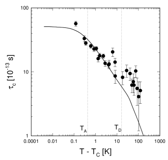
FIG. 2.: Experimental and theoretical results of the autocorrelation time $\tau_{c}$ for PAC-experiments. Data taken from [1].

Let us now compare the results of our mode coupling theory with hyperfine experiments on Gd mentioned above [1, 2, 3]. The autocorrelation time $\tau_{c}$ is shown in Figs. 2 and 3 for PAC experiments and Moessbauer spectroscopy, respectively. Both sets of data are in excellent agreement with the results from mode coupling theory for $T-T_{c}<10K$. Note that besides the overall frequency scale there is no fit-parameter, since we have used the same set of values for the dipolar and uniaxial wave vector as for our comparison with $\mu$SR experiments.

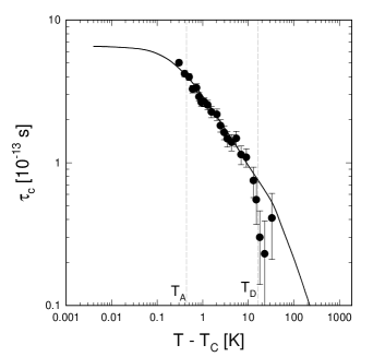
FIG. 3.: Experimental and theoretical results of the autocorrelation time $\tau_{c}$ for Moessbauer spectroscopy experiments. Data taken from [2, 3].

In summary, we have outlined a mode coupling theory for uniaxial dipolar ferromagnets, where the uniaxiality solely results from the dipolar interaction. We have also reported measurements on a high purity single crystal sample of gadolinium metal in the paramagnetic regime. From the quantitative agreement between this theory and our $\mu$SR and previous PAC and Moessbauer measurements the following conclusions can be drawn: (i) The universality class of Gd is the uniaxial dipolar ferromagnet, where both the isotropic dipolar and the uniaxial contribution to the spin Hamiltonian are due to a combined effect of dipolar interaction and non-cubic lattice structure. This corresponds to a new anisotropic model J^∗, where the Hamiltonian is given by Eq. 4. (ii) The dominant factor for the uniaxial anisotropy in Gd is the dipolar interaction. (iii) Muons in Gd are located at octrahedral interstitial sites close to $T_{c}$.

Acknowledgment: It is a pleasure to acknowledge helpful discussions with A. Yaouanc and P. Dalmas de Réotier. This work has been supported by the German Federal Ministry for Education and Research under Contract No. 03SC4TUM and No. 03KA2TUM4. E.F. acknowledges support from the Deutsche Forschungsgemeinschaft under Contract No. Fr. 850/2.

REFERENCES

- [1] G. Collins, A. Chowdhury, and C. Hohenemser, Phys. Rev. B 33, 4747 (1986).
- [2] A. Chowdhury, G. Collins, and C. Hohenemser, Phys. Rev. B 30, 6277 (1984).
- [3] A. Chowdhury, G. Collins, and C. Hohenemser, Phys. Rev. B 33, 5070 (1986).
- [4] O. Hartmann et al., Hyperf. Int. 64, 369 (1990).
- [5] E. Wäckelgard et al., Hyperf. Int. 31, 325 (1986).
- [6] E. Wäckelgard et al., Hyperf. Int. 50, 781 (1989).
- [7] D. Geldart, P. Hargraves, N. Fujiki, and R. Dunlap, Phys. Rev. Lett. 62, 2728 (1989).
- [8] P. Hohenberg and B. Halperin, Rev. Mod. Phys. 49, 435 (1977).
- [9] J. Cable and E. Wollan, Physical Review 165, 733 (1968).
- [10] N. Fujiki, K. De’Bell, and D. Geldart, Phys. Rev. B 36, 8512 (1987).
- [11] A. Aharony and M. Fisher, Phys. Rev. B 8, 3323 (1973).
- [12] E. Frey and F. Schwabl, Adv. Phys. 43, 577 (1994).
- [13] S. Henneberger, E. Frey, F. Schwabl, and G. Kalvius, (unpublished).
- [14] K. Ried, Y. Millev, M. Fähnle, and H. Kronmüller, Phys. Rev. B 51, 15229 (1996).
- [15] C. Bagnuls and C. Joukoff-Piette, Phys. Rev. B 11, 1986 (1975).
- [16] S. Henneberger et al., Hyperf. Int. 104, 301 (1997).
- [17] A. Yaouanc, P. D. de Réotier, and E. Frey, Phys. Rev. B 50, 3033 (1994).
- [18] P. D. de Réotier and A. Yaouanc, Phys. Rev. Lett. 72, 290 (1994).
- [19] A. Denison, H. Graf, W. Kündig, and P. Meier, Helv. Phys. Acta 52, 460 (1979).