[

Flexive and Propulsive Dynamics of Elastica at Low Reynolds Numbers

Abstract

A stiff one-armed swimmer in glycerine goes nowhere, but if its arm is elastic, exerting a restorative torque proportional to local curvature, the swimmer can go on its way. Considering this happy consequence and the principles of elasticity, we study a hyperdiffusion equation for the shape of the elastica in viscous flow, find solutions for impulsive or oscillatory forcing, and elucidate relevant aspects of propulsion. These results have application in a variety of physical and biological contexts, from dynamic biopolymer bending experiments to instabilities of elastic filaments.

]

In Stokes flow, the Aristotelian fluid regime inhabited by the very small or the very slow, inertia is irrelevant. This fact underlies the inability of a variety of swimming motions, perfectly successful on human scales, to generate net motion on microscopic scales [1]. An oft-quoted example is the lack of propulsion for a swimmer with only one degree of mechanical freedom, e.g. the paradigmatic scallop of Purcell’s 1977 lecture which introduced many to the principles of Stokes flow [2]. Colloquially known as “the scallop theorem,” this observation derives from the more general statement that motions invariant under $t\rightarrow-t$ can produce no net effect [1]; movies of Stokes flow must appear equally sensible when reversed [3].

Purcell observed two ways to elude the scallop theorem: rotate a chiral arm, or wave an elastic arm. While the former dynamic is well-studied (most notably, in the context of E. coli [4]), the latter is largely uninvestigated [5], despite its relation to experiments from motility assays to dynamic studies of biopolymer bending moduli. To elucidate this dynamic, we here study the motion of a one-armed swimmer with an elastic prosthesis, or equivalently a driven elastic filament. Building on experiments showing the hyperdiffusivity of small-amplitude planar deformations [6], we quantify how an elastic filament eludes the scallop theorem, suggest experiments to test these results, and show how this analysis allows for the measurment of bending moduli. Remarkably, the required mathematics [7] is central to an intrinsic description of overdamped elastica in three dimensions.

Force-velocity proportionalities in Stokes flow are generally not simple; notable exceptions are for highly symmetric objects such as the sphere ($F=6\pi\mu av$, with $a$ the radius), and those for which length $L$ greatly exceeds width $d$, where slender-body hydrodynamics [8, 9] applies. To lowest order in $1/\ln(L/d)$, force and velocity obey a local, anisotropic proportionality. For velocity $v$ normal to the long axis, the force per unit length $f=\zeta v$, with $\zeta=4\pi\mu/(\ln(L/d)+c)$, where $c$ is an ${\cal O}(1)$ constant determined by the shape of the object. For an elastic filament with bending modulus $A$, $-f$ is the functional derivative of the bending energy $A/2\int_{0}^{L}dx~{}y_{xx}^{2}$, written here for small planar deformations $y(x)$; thus, $f=-Ay_{xxxx}$. At free ends the functional derivative implies boundary conditions of torquelessness and forcelessness: $y_{xx}=y_{xxx}=0$. For small deformations $v=y_{t}$, and with the hyperdiffusion constant ${\tilde{\nu}}=A/\zeta$, we have

$$y_{t}=-{\tilde{\nu}}y_{xxxx}~{},$$ (1)

perhaps the simplest model for the balance between viscous drag and bending elasticity.

In 1851, Stokes suggested two problems in fluid mechanics, here termed SI and SII (Fig. 1), to illustrate viscous diffusion of velocity [10]: SI - impulsively move a wall bounding a fluid; SII - oscillate the wall at frequency $\omega$. These motivate two problems for the elastohydrodynamic equation of motion (1): EHDI - impulsively move one end of a filament; EHDII - oscillate the end. In SI and SII, the Navier-Stokes equation reduces to a diffusion equation $u_{t}=\nu u_{xx}$, with kinematic viscosity $\nu=\mu/\rho$. For a semi-infinite domain, the post-transient solution of SII consists of decaying, right-moving waves, $u\left(x,t\right)=U\exp(-\eta/\sqrt{2})\cos\left(\eta/\sqrt{2}-\omega t\right)$, with $\eta=x/\ell_{\nu}$, and viscous penetration length $\ell_{\nu}=(\nu/\omega)^{1/2}$. In EHDII the analogous elastohydrodynamic penetration length is

$$\ell_{{\tilde{\nu}}}(\omega)=\left({{\tilde{\nu}}/\omega}\right)^{1/4}.$$ (2)

FIG. 1.: Geometry of Stokes problems I and II (left) and of elastohydrodynamic problems I and II (right).

Imposing the left filament end position $y_{0}\cos\omega t$ and torquelessness for the left end [11] $y_{xx}(0,t)=0$, we find

$${y\over y_{0}}={1\over 2}\Bigl{[}{\rm e}^{-\tilde{C}\eta}\cos\left(\tilde{S}\eta+\omega t\right)+{\rm e}^{-\tilde{S}\eta}\cos\left(\tilde{C}\eta-\omega t\right)\Bigr{]},$$ (3)

where $\tilde{C}=\cos\left(\pi/8\right)$, $\tilde{S}=\sin\left(\pi/8\right)$, and now $\eta=x/\ell_{{\tilde{\nu}}}$. Unlike SII, EHDII supports left- and right-moving waves (with different velocities and decay lengths), despite the lack of a reflecting right-end boundary.

For finite filaments we define a rescaled length ${\cal L}\equiv L/\ell_{{\tilde{\nu}}}(\omega)$ and coordinate $\alpha=x/L$. When ${\cal L}\lesssim 1$ the filament behaves as a rigid rod, while it undulates appreciably for ${\cal L}\gg 1$. In this way $\ell_{{\tilde{\nu}}}$ resembles the persistence length $L_{p}$. The exact solution of EHDII for finite $L$ [7] has an expansion in powers of ${\cal L}^{4}$ whose first terms are

$${y\over y_{0}} \simeq \left(1-{3\over 2}\alpha\right)\cos(\omega t)+{{\cal L}^{4}\over 1680}\bigl{(}16\alpha-70\alpha^{3}$$ (5)

$$+70\alpha^{4}-21\alpha^{5}\bigr{)}\sin(\omega t)+{\cal O}({\cal L}^{8})~{}.$$

At order ${\cal L}^{0}$, the filament is a straight rod that interestingly pivots about a point two-thirds of its length. Flexive corrections at ${\cal O}({\cal L}^{4})$ break time-reversal invariance. Solutions of increasing ${\cal L}$ are shown in Fig. 2, whose inset shows the results of an experiment on actin [6] in which observed shapes in a range of frequencies were fit for $\ell_{{\tilde{\nu}}}$ to the exact expressions [7], verifying the scaling $\ell_{{\tilde{\nu}}}\sim\omega^{-1/4}$ as well as providing a novel dynamic technique for measuring the bending modulus $A$.

The propulsive force $F_{x}$ imparted to the fluid by the filament (or vice versa) may be computed by integrating the projected elastic force density ${\bf f}\cdot\hat{\bf e}_{x}$ along the filament. Interestingly, with the boundary conditions of EHDII and the geometrically exact form of ${\bf f}$ this result is expressible

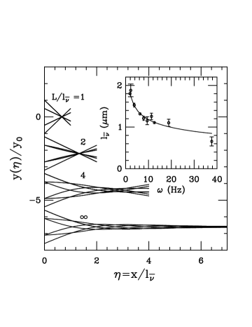
FIG. 2.: Solutions to (1) for oscillatory driving at various rescaled lengths ${\cal L}=L/\ell_{{\tilde{\nu}}}$. Inset: experimental verification [6] of the frequency dependence of $\ell_{{\tilde{\nu}}}(\omega)$ yielding a modulus $A/k_{B}T=7.4\mu$m, well within the range ($0.5\mu$m [12] to $17\mu$m [13]) of measurements employing statistical techniques.

in terms of the curvature $\kappa$ and tangent angle $\theta$ at the forcing point: $F_{x}=A\kappa_{s}\sin\theta(s=0)\simeq Ay_{x}y_{xxx}(x=0)$. The time average of this quantity over one period gives

$$\bar{F}_{x}={y_{0}^{2}\zeta|\omega|\over 4\sqrt{2}}Y\left({\cal L}\right)~{}$$ (6)

For ${\cal L}\ll 1$, $Y\simeq(11/3360){\cal L}^{4}$, so $\bar{F}_{x}\sim y_{0}^{2}\zeta^{2}\omega^{2}L^{4}/A$; a short (or infinitely stiff) pivoting filament produces no net force (by the scallop theorem). Flexibility leads to a net leftward propulsion, as the right-moving waves dominate the left-movers. An unexpected, fascinating feature (Fig. 3) is the maximum in $Y$ indicating an optimal value of the length $L^{*}\simeq 4.07(A/\zeta\omega)^{1/4}$.

In a familiar way, this force is associated with the trajectory of the filament shape in a low-dimensional projection of configuration space. The relation $F(t)=Ay_{x}(0,t)y_{xxx}(0,t)$ and the equation of motion imply

$$\bar{F}_{x}={\zeta\omega\over 2\pi}\int_{0}^{2\pi/\omega}\!\!dty_{x}(0,t){\partial\over\partial t}\int_{0}^{L}\!\!dxy={\zeta\omega\over 2\pi}\oint\theta_{0}d{\mathcal{A}}~{},$$ (7)

where ${\mathcal{A}}$ is the area under the curve $y(x)$ and $\theta_{0}\simeq y_{x}$ is the tangent angle at the left end. Thus, the net force during the cyclic motion is the area enclosed in the associated ‘Carnot diagram’ in ${\mathcal{A}}-\theta_{0}$ space; it results from pushing aside some volume of fluid (area, in two dimensions), projected via $\theta_{0}$ in the direction of propulsion. For EHDII, the trajectory is an ellipse; it thins to a straight line for the time-reversible pivoting of a rod, encloses no area, and thus produces no force. Observe the intuitive result that net propulsion in the transverse direction, proportional to $\oint d{\mathcal{A}}=0$, vanishes identically.

We estimate the efficiency ${\cal E}$ of this motion [1] by comparing the power $P_{\parallel}=\bar{F}_{x}v_{x}\simeq\bar{F}_{x}^{2}/L\zeta_{\parallel}$ for longitudinal propulsion to the power $P_{\perp}=F_{y}v_{y}\simeq\int ds\zeta_{\perp}y_{t}^{2}$ dissipated in transverse motions, to obtain

$${\cal E}=\left({y_{0}\over 2\ell_{{\tilde{\nu}}}}\right)^{2}{\zeta_{\perp}\over\zeta_{\parallel}}Z\left({\cal L}\right)~{},$$ (8)

where $Z({\cal L})$ is the scaling function shown in the inset to Fig. 3. Filaments short relative to $\ell_{\tilde{\nu}}(\omega)$ flex little and produce little propulsion, while long ones have excess drag from the nearly straight regions far away from the point of forcing, yielding a sharp maximum at ${\cal L}\sim 4.0$.

These observations suggest experiments in the spirit of those by Taylor [14] on swimming with a helical flagellum. Exploiting the results of EHDII, perhaps carried out on microfilaments with laser [6] or magnetic tweezers, or on macroscopic objects, one might measure the propulsive force through the transverse displacement at the forcing point, test for the predicted maximum as a function of frequency, investigate the role of nonlinearities, and study interactions between flexing filaments. Analogous experiments incorporating twist (perhaps via magnetic optically-trapped beads, as in [15]) could elucidate instabilities exhibited by helical motion of flexible filaments [16] and associated propulsion.

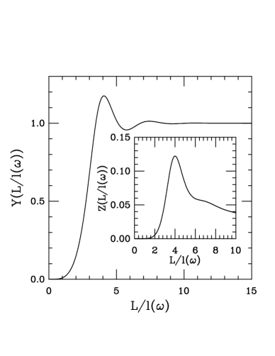
FIG. 3.: Scaling functions $Y$, for propulsive force, and $Z$, for efficiency, versus rescaled length ${\cal L}=L/\ell_{{\tilde{\nu}}}(\omega)$.

A swimmer’s arm may also move by discrete, noncyclic strokes. The associated model dynamic (EHDI) is the relaxation of a filament to an equilibrium shape given some boundary condition at the point of attachment. Since (1) is linear, we may subtract from its general solution a particular solution consistent with nonzero boundary conditions or external driving to obtain a homogeneous problem with $0$-valued boundary conditions. This motivates the construction of a self-adjoint operator from ${\cal H}\equiv\partial_{x}^{4}$, whose well-known eigenfunctions are

$${\cal W}_{q}(x) = a_{1}\sin\left(qx\right)+a_{2}\cos\left(qx\right)$$ (10)

$$+a_{3}\sinh\left(qx\right)+a_{4}\cosh\left(qx\right)~{},$$

where ${\cal H}{\cal W}_{q}=q^{4}{\cal W}_{q}$. The ten distinct choices of boundary conditions for which $\cal H$ is self adjoint [7] determine the distinct coefficients $\{a_{i}\}$ of ${\cal W}_{q}$ and the allowed wavenumbers $q$. These $q$ are roots of transendental solvability conditions; certain boundary conditions are satisfied by Fourier modes (those for which $a_{3}=a_{4}=0$).

The completeness of the set ${\cal W}_{q}$ yields the homogeneous solution to (1),

$$y(x,t)=\sum_{q}{\cal W}_{q}(x){\rm e}^{-{\tilde{\nu}}q^{4}t}\int_{0}^{L}dx{\cal W}_{q}(x)y(x,0)~{},$$ (11)

relevant to a second class of techniques for measuring bending moduli. One recent example [17] is the relaxation of the free end of an initially bent microtubule whose opposite end is clamped to a cover slip via the axoneme from which it is nucleated. Using typical material parameters for microtubules, ($L\sim\mu$m, $\zeta\sim$ cP, $L_{p}\sim$ mm), we observe from (11) that beyond the inital few milliseconds the filament straightens with a time constant $\tau_{1}=1/{\tilde{\nu}}q_{1}^{4}$; here $q_{1}\simeq 1.875/L$ the smallest root of the clamped-free solvability condition $\cos(qL)\cosh(qL)=-1$ [18]. Measurement of $\tau_{1}$ gives $A$.

Finally, we apply these results to an important subject in pattern formation: intrinsic formulations of filament motion [19] and their extention to nonplanar dynamics. The dynamical evolution of the Frenet-Serret (FS) curvature $\kappa$ and torsion $\tau$ are singular at inflection points (where $\kappa=0$ and $\tau$ is undefined), a problem removed by instead using the parameterization [20, 21]

$$\psi(s,t)=\kappa(s,t){\rm e}^{i\phi(s,t)}~{},\ \ \ \ {\bf w}=(\hat{\bf n}+i\hat{\bf b}){\rm e}^{i\phi}~{},$$ (12)

where $\phi(s,t)=\int^{s}\!\!ds^{\prime}\tau(s^{\prime},t)$, and $\hat{\bf n}$ and $\hat{\bf b}$ are the normal and binormal vectors. Across an inflection point at, say, $s=0$, the normal and binormal vectors $\hat{\bf n}$ and $\hat{\bf b}$ flip sign, the torsion has a singular piece, $\tau=\pi\delta(s)$, so there is a discontinuity $\phi(0^{+})-\phi(0^{-})=\pi$. Yet, this leaves ${\bf w}$ and $\psi$ continuous. The curve ${\bf r}(s)$ is constructed from $\psi$ via new FS equations: ${\bf w}_{s}=-\psi\hat{\bf t};\ \hat{\bf t}_{s}={\rm Re}(\psi^{*}{\bf w})$. Some elementary shapes have very simple $\psi$-representations: the straight line $\psi=0$, the circle $\psi=a$, the helix $\psi=a{\rm e}^{ips}$ ($a,p$ constant).

The intrinsic inextensible evolution for $\psi$ [20],

$$\psi_{t}=(\partial_{ss}+|\psi|^{2})\Upsilon+\psi{\rm Im}\int^{s}\!\!ds^{\prime}\psi_{s}\Upsilon^{*}+W\psi_{s}~{},$$ (13)

depends upon the velocity components ${\bf r}_{t}=U\hat{\bf n}+V\hat{\bf b}+W\hat{\bf t}$ through the complex velocity $\Upsilon=(U+iV){\rm e}^{i\phi}$. It can be shown [22] from the governing equations for viscous motion of filaments, that $\Upsilon=-{\tilde{\nu}}(\psi_{ss}+(1/2)|\psi|^{2}\psi)$. Thus, the $\psi$ dynamics is hyperdiffusive as in (1) [20],

$$\psi_{t}\simeq-{\tilde{\nu}}\psi_{ssss}+\cdots~{}.$$ (14)

For an elastic energy ${\cal E}=(A/2)\int\!ds\kappa^{2}$ the boundary conditions at free ends are $\kappa=\kappa_{s}=\kappa\tau=0$, or simply $\psi=\psi_{s}=0$. Since the self-adjoint operator is again ${\cal H}=\partial_{s}^{4}$, the ${\cal W}_{q}(s)$, now functions of arclength, are the relevant eigenfunctions. Thus, the $\psi$ formulation, the natural singularity-free mathematical representation of the curve, also compactly encodes the physical boundary conditions and dynamics. Since the ${\cal W}_{q}$ form a complete set, the evolving shape of any filament is expressible as

$\displaystyle\psi(s,t)=\sum_{q}c_{q}(t){\cal W}_{q}(s)~{},$the time evolution being a nonlinear dynamical system in $c_{q}(t)\equiv\langle{\cal W}_{q}|\psi(s,t)\rangle$; in the linearized regime, $c_{q}(t)=c_{q}(0)\exp(-{\tilde{\nu}}q^{4}t)$. The modes ${\cal W}_{q}$ are like the Rouse modes of a flexible polymer, and the “clamped” eigenfunctions of $y_{t}=-{\tilde{\nu}}y_{xxxx}$ (with $y=y_{x}=0$ at $x=0,L$) are the “free” eigenfunctions of $\psi_{t}=-{\tilde{\nu}}\psi_{ssss}$, with $\cos(qL)\cosh(qL)=1$. The first three are shown in Fig. 4. When the complex coefficients $c_{q}$ share a common phase the curve is planar, otherwise it has torsion. The latter case is shown in Fig. 4 as a coiled three-dimensional filament composed of the first two modes, reconstructed from the complex FS equations. The simplification achieved with the $\psi$ formulation is clear.

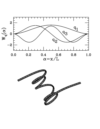
FIG. 4.: Biharmonic eigenfunctions and a nonplanar elastica. Top: ${\cal W}_{q}$ with boundary conditions ${\cal W}=\partial_{\alpha}{\cal W}=0$. Bottom: free filament with $\psi=15({\cal W}_{q_{1}}+i{\cal W}_{q_{2}})$.

This formalism easily generalizes to twisted filaments [22], as found for instance in bacterial systems that undergo hierarchical buckling and writhing instabilities [23]. For a constant twist density $\Omega$ and twist elastic constant $C$ the moment relation ${\bf M}=A\kappa\hat{\bf b}+C\Omega\hat{\bf t}$ can be shown to yield the complex velocity [24]

$$\Upsilon=-{\tilde{\nu}}(\psi_{ss}+{1\over 2}|\psi|^{2}\psi)+i{\tilde{\nu}}C\Omega\psi_{s}~{},$$ (15)

so the intrinsic dynamics (14) is explicitly complex

$$\psi_{t}\simeq-{\tilde{\nu}}(\psi_{ssss}+i\Omega\Gamma\psi_{sss})+\cdots~{},$$ (16)

with $\Gamma=C/A$. A helical perturbation $\psi\sim\exp(iks+\sigma t)$ to a straight filament leads to a growth rate $\sigma=-{\tilde{\nu}}(k^{4}+\Gamma\Omega k^{3})$. This describes a writhing instability on a length scale $L_{Wr}=2\pi/\Omega\Gamma$ to a helix whose handedness is set by the sign of the twist density $\Omega$. A stability analysis [22] about a loop of radius $R$ yields not only the criterion $\Gamma\Omega R=\sqrt{3}$ for the onset of the primary instability [25], but also the growth rates $\sigma_{\pm}$ for the coupled bending and writhing modes. Extensions to the fully nonlinear regime are then straightforward, leading to a “dynamics of twist and writhe” that complements important existing Hamiltonian formulations [26].

We thank A. Ott and D.X. Riveline for collaborations, S. Childress, J. Kessler, and C. O’Hern for discussions and R. Kamien, P. Nelson, and T. Powers for insightful and instructive protests. This work was supported by an NSF Presidential Faculty Fellowship, DMR 96-96257 (REG). This paper is dedicated to the late E. Purcell.

REFERENCES

- [1] S. Childress, Swimming and Flying in Nature. (Cambridge, Cambridge University Press, 1981).
- [2] E. M. Purcell, Am. J. Phys. 45, 3 (1977).
- [3] “Low Reynolds Number Flows” (film). Encyclopædia Brittanica Educational Corporation. 1966.
- [4] Lighthill, Sir J. 1975. Mathematical Biofluiddynamics. SIAM, Philadelphia.
- [5] Early work is K.E. Machin, J. Exp. Biol. 35, 796 (1958). We are here addressing the passive rather than active flagellum, the latter an area of great activity[1, 4].
- [6] D. Riveline, C.H. Wiggins, R.E. Goldstein, A. Ott, Phys. Rev. E. 56, 1330 (1997).
- [7] C. Wiggins, D. Riveline, R. Goldstein, and A. Ott, “Trapping and Wiggling: Elastohydrodynamics of Driven Microfilaments,” submitted to Biophys. J. (1997).
- [8] R.G. Cox, J. Fluid Mech. 44, 791 (1970); 45, 625 (1970).
- [9] J. Keller and S. Rubinow, J. Fluid Mech. 75, 705 (1976).
- [10] G.G. Stokes, Trans. Camb. Phil. Soc. 9, 8 (1851).
- [11] The condition of torquelessness holds for a filament attached to a bead held in an optical trap as in [6].
- [12] J. Käs, H. Strey, M. Baermann, and E. Sackmann, Europhys. Lett. 21, 865 (1993).
- [13] A. Ott, M. Magnasco, A. Simon, and A. Libchaber, Phys. Rev. E 48, 1642 (1993).
- [14] G.I. Taylor, Proc. Roy. Soc. A 211, 225 (1952).
- [15] T.R. Strick, J.-F. Allemand, D. Bensimon, A. Bensimon, and V. Croquette, Science 271, 1835 (1996).
- [16] We thank P. Nelson for this suggestion.
- [17] H. Felgner, R. Frank, and M. Schliwa, J. Cell Science 109, 509 (1996).
- [18] See also F. Gittes, B. Mickey, J. Nettleton, and J. Howard, J. Cell Biol. 120, 923 (1993).
- [19] M.J. Shelley and T. Ueda, in Advances in Multi-fluid Flows, Y. Y. Renardy, et al., eds. (Philadelphia, AMS-SIAM, 1996), p. 415; T. Y. Hou, J. S. Lowengrub, and M. J. Shelley, J. Comp. Phys. 114, 312 (1994).
- [20] R.E. Goldstein and S.A. Langer, Phys. Rev. Lett. 75, 1094 (1995).
- [21] H. Hasimoto, J. Fluid Mech. 51, 477 (1972); G. Darboux, Leçons sur la Théorie Genérale des Surfaces (Gauthier-Villars, Paris, 1915), Vol. I, p. 22.
- [22] C.H. Wiggins, et al., unpublished (1997).
- [23] N.H. Mendelson, Microbiol. Rev. 46, 341 (1982).
- [24] See also Y. Shi and J.E. Hearst, J. Chem. Phys. 101, 5186 (1994).
- [25] E.E. Zajac, Trans. ASME, March, 136 (1962).
- [26] A. Goriely and M. Tabor, Physica D. 105, 20 (1997).