Surface Critical Behavior of bcc Binary Alloys

Abstract

The surface critical behavior of bcc binary alloys undergoing a continuous $B2$-$A2$ order-disorder transition in the bulk is investigated in the mean-field (MF) approximation, employing a semi-infinite lattice model equivalent to an Ising antiferromagnet in an external field. Our main aim is to present clear evidence for the fact that surfaces which break the two-sublattice symmetry generically display the critical behavior of the normal transition, whereas symmetry-preserving surfaces exhibit the behavior of the ordinary transition. To this end, the lattice MF equations for both symmetry-breaking (100) and symmetry-preserving (110) surfaces are cast in the form of nonlinear symplectic maps, the associated Hamiltonian flows are analyzed, and the length scales involved are computed. Careful examination of the continuum limit yields the appropriate semi-infinite Ginzburg-Landau model for the (100) surface and reveals subtleties overlooked in previous work. The continuum model involves an “effective” ordering surface field $g_{1}\neq 0$, which depends on the parameters of the lattice model. The singular behavior predicted by the Ginzburg-Landau model is shown to agree quantitatively with the solutions of the lattice MF equations.

I Introduction

Experiments on binary ($AB$) alloys that undergo an order-disorder transition in the bulk have yielded a wealth of information on surface critical phenomena in semi-infinite matter.[1] In these systems one inevitably has to cope with the influence of surface segregation, i. e., the enrichment of one component at the surface. Surface segregation occurs, e. g., due to different interaction energies or sizes of the two species. Theoretically, the variation of the local composition near the surface may necessitate the introduction of “nonordering” densities, which are given by linear combinations of the local concentrations of $A$ and $B$ atoms on the various sublattices. In the case of surface critical phenomena at first-order bulk transitions, such as “surface-induced disordering” in fcc binary alloys, nonordering densities strongly influence the asymptotic behavior.[2] In this paper we are concerned with bcc alloys that exhibit a continuous (second-order) bulk transition and are thus promising candidates for testing current theories of surface critical behavior at bulk critical points.[3, 4, 5]

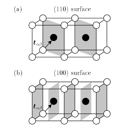
FIG. 1.: Examples of (a) symmetry-preserving, and (b) symmetry-breaking surfaces. Sites of sublattices $\alpha$ and $\beta$ correspond to open and full circles, respectively. In the $A2$ phase, the concentration of either component is the same on all sites, whereas the two sublattices are preferentially occupied by $A$ and $B$ atoms, respectively, in the ordered $B2$ phase.

The continuous $B2$-$A2$ transition occurring in FeAl or FeCo has been investigated previously by F. Schmid.[6] She studied a semi-infinite lattice model equivalent to a bcc Ising antiferromagnet both by Monte Carlo simulation and within the mean-field (MF) approximation, and made the important observation that the orientation of the surface in general matters. Her conclusions can be summarized as follows: (a) A nonvanishing order parameter (OP) profile occurs for $T\geq T_{c}$, the bulk critical temperature, provided that (i) the surface breaks the two-sublattice symmetry (see below), and (ii) one component is enriched at the surface. (b^′) The observable surface critical behavior should be representative of the ordinary universality class even if the above conditions (i) and (ii) are met.

While we agree with (a), we find that (b^′) should be replaced by (b): If conditions (i) and (ii) are satisfied, the surface critical behavior generically is characteristic of the normal transition, which belongs to the same universality class as the extraordinary transition.[7]

In a foregoing Letter [8] by Drewitz, Burkhardt, and ourselves, exact transfer matrix calculations were employed in conjunction with conformal invariance to present clear evidence for (a) and (b) in bulk dimension $d=2$. Here we generalize these results to arbitrary $d$ using MF theory and a mapping onto a Ginzburg-Landau model.

The reason for the appearance of normal critical behavior is a subtle interplay between the symmetry with respect to sublattice ordering and broken translational invariance due to the free surface. Consider first a finite system with periodic boundary conditions. The precise form of the Hamiltonian ${\cal H}\{\sigma_{\mathchoice{{\hbox{\boldmath$\displaystyle i$}}}{{\hbox{\boldmath$\textstyle i$}}}{{\hbox{\boldmath$\scriptstyle i$}}}{{\hbox{\boldmath$\scriptscriptstyle i$}}}}\}$ does not matter here and will be given in Sec. II. The spin variable $\sigma_{\mathchoice{{\hbox{\boldmath$\displaystyle i$}}}{{\hbox{\boldmath$\textstyle i$}}}{{\hbox{\boldmath$\scriptstyle i$}}}{{\hbox{\boldmath$\scriptscriptstyle i$}}}}=1$ ($\sigma_{\mathchoice{{\hbox{\boldmath$\displaystyle i$}}}{{\hbox{\boldmath$\textstyle i$}}}{{\hbox{\boldmath$\scriptstyle i$}}}{{\hbox{\boldmath$\scriptscriptstyle i$}}}}=-1$) represents an $A$ ($B$) atom on lattice site $\textstyle i$. The statistical weight of a configuration $\{\sigma_{\mathchoice{{\hbox{\boldmath$\displaystyle i$}}}{{\hbox{\boldmath$\textstyle i$}}}{{\hbox{\boldmath$\scriptstyle i$}}}{{\hbox{\boldmath$\scriptscriptstyle i$}}}}\}$ is given by the finite-volume Gibbs measure

$$\rho(\{\sigma_{\mathchoice{{\hbox{\boldmath$\displaystyle i$}}}{{\hbox{\boldmath$\textstyle i$}}}{{\hbox{\boldmath$\scriptstyle i$}}}{{\hbox{\boldmath$\scriptscriptstyle i$}}}}\})=\frac{1}{Z}e^{-\beta{\cal H}\{\sigma_{\mathchoice{{\hbox{\boldmath$\displaystyle i$}}}{{\hbox{\boldmath$\textstyle i$}}}{{\hbox{\boldmath$\scriptstyle i$}}}{{\hbox{\boldmath$\scriptscriptstyle i$}}}}\}}\,,\quad\beta\equiv 1/(k_{B}T)\,,$$ (1)

where $T$ is the temperature and $k_{B}$ denotes Boltzmann’s constant. The normalization factor $Z$ is the grand-canonical partition function. The local concentration $c_{\mathchoice{{\hbox{\boldmath$\displaystyle i$}}}{{\hbox{\boldmath$\textstyle i$}}}{{\hbox{\boldmath$\scriptstyle i$}}}{{\hbox{\boldmath$\scriptscriptstyle i$}}}}$ of $A$ atoms at site $\textstyle i$ can be expressed in terms of the mean magnetization $\langle\sigma_{\mathchoice{{\hbox{\boldmath$\displaystyle i$}}}{{\hbox{\boldmath$\textstyle i$}}}{{\hbox{\boldmath$\scriptstyle i$}}}{{\hbox{\boldmath$\scriptscriptstyle i$}}}}\rangle$ as $c_{\mathchoice{{\hbox{\boldmath$\displaystyle i$}}}{{\hbox{\boldmath$\textstyle i$}}}{{\hbox{\boldmath$\scriptstyle i$}}}{{\hbox{\boldmath$\scriptscriptstyle i$}}}}=(1+\langle\sigma_{\mathchoice{{\hbox{\boldmath$\displaystyle i$}}}{{\hbox{\boldmath$\textstyle i$}}}{{\hbox{\boldmath$\scriptstyle i$}}}{{\hbox{\boldmath$\scriptscriptstyle i$}}}}\rangle)/2$. The Gibbs measure (1) is translationally invariant,

$$\rho(\{\sigma_{\mathchoice{{\hbox{\boldmath$\displaystyle i$}}}{{\hbox{\boldmath$\textstyle i$}}}{{\hbox{\boldmath$\scriptstyle i$}}}{{\hbox{\boldmath$\scriptscriptstyle i$}}}}\})=\rho(\{\sigma_{\mathchoice{{\hbox{\boldmath$\displaystyle i$}}}{{\hbox{\boldmath$\textstyle i$}}}{{\hbox{\boldmath$\scriptstyle i$}}}{{\hbox{\boldmath$\scriptscriptstyle i$}}}}^{\prime}\})\,,\quad\sigma_{\mathchoice{{\hbox{\boldmath$\displaystyle i$}}}{{\hbox{\boldmath$\textstyle i$}}}{{\hbox{\boldmath$\scriptstyle i$}}}{{\hbox{\boldmath$\scriptscriptstyle i$}}}}^{\prime}\equiv\sigma_{\mathchoice{{\hbox{\boldmath$\displaystyle i$}}}{{\hbox{\boldmath$\textstyle i$}}}{{\hbox{\boldmath$\scriptstyle i$}}}{{\hbox{\boldmath$\scriptscriptstyle i$}}}+\mathchoice{{\hbox{\boldmath$\displaystyle t$}}}{{\hbox{\boldmath$\textstyle t$}}}{{\hbox{\boldmath$\scriptstyle t$}}}{{\hbox{\boldmath$\scriptscriptstyle t$}}}}\,,$$ (2)

where $\textstyle t$ may be chosen arbitrarily from the set $\cal T$ of all bcc lattice vectors. Due to spontaneous symmetry breaking, the thermodynamic states that are obtained by calculating expectation values with the measure (1) and taking the infinite-volume limit need not be translationally invariant. (Formally, one introduces a symmetry-breaking “staggered” field which is sent to zero after the thermodynamic limit has been performed.) In the ordered phase below $T_{c}$, one has $\langle\sigma_{\mathchoice{{\hbox{\boldmath$\displaystyle i$}}}{{\hbox{\boldmath$\textstyle i$}}}{{\hbox{\boldmath$\scriptstyle i$}}}{{\hbox{\boldmath$\scriptscriptstyle i$}}}}\rangle\neq\langle\sigma_{\mathchoice{{\hbox{\boldmath$\displaystyle i$}}}{{\hbox{\boldmath$\textstyle i$}}}{{\hbox{\boldmath$\scriptstyle i$}}}{{\hbox{\boldmath$\scriptscriptstyle i$}}}+\mathchoice{{\hbox{\boldmath$\displaystyle t$}}}{{\hbox{\boldmath$\textstyle t$}}}{{\hbox{\boldmath$\scriptstyle t$}}}{{\hbox{\boldmath$\scriptscriptstyle t$}}}}\rangle$ for all translations $\mathchoice{{\hbox{\boldmath$\displaystyle t$}}}{{\hbox{\boldmath$\textstyle t$}}}{{\hbox{\boldmath$\scriptstyle t$}}}{{\hbox{\boldmath$\scriptscriptstyle t$}}}=\mathchoice{{\hbox{\boldmath$\displaystyle t$}}}{{\hbox{\boldmath$\textstyle t$}}}{{\hbox{\boldmath$\scriptstyle t$}}}{{\hbox{\boldmath$\scriptscriptstyle t$}}}_{\alpha\beta}$ that map $\alpha$ to $\beta$-sites (Fig. 1).

Surfaces are introduced by imposing free boundary conditions along one direction while retaining periodic boundary conditions in the other directions. Then the measure (1) is invariant under the subset ${\cal T}^{\prime}\subset{\cal T}$ of translations parallel to the surface. We call the surface symmetry-preserving if ${\cal T}^{\prime}$ contains a “sublattice-exchanging” translation $\mathchoice{{\hbox{\boldmath$\displaystyle t$}}}{{\hbox{\boldmath$\textstyle t$}}}{{\hbox{\boldmath$\scriptstyle t$}}}{{\hbox{\boldmath$\scriptscriptstyle t$}}}_{\alpha\beta}$, and symmetry-breaking otherwise. In the case of the bcc lattice considered here, symmetry-breaking surfaces are characterized by the alternation of $\alpha$ and $\beta$-planes along the direction normal to the surface. Let us assume that no spontaneous symmetry breaking takes place above $T_{c}$, which would require supercritically enhanced surface couplings, so that $\langle\sigma_{\mathchoice{{\hbox{\boldmath$\displaystyle i$}}}{{\hbox{\boldmath$\textstyle i$}}}{{\hbox{\boldmath$\scriptstyle i$}}}{{\hbox{\boldmath$\scriptscriptstyle i$}}}}\rangle=\langle\sigma_{\mathchoice{{\hbox{\boldmath$\displaystyle i$}}}{{\hbox{\boldmath$\textstyle i$}}}{{\hbox{\boldmath$\scriptstyle i$}}}{{\hbox{\boldmath$\scriptscriptstyle i$}}}+\mathchoice{{\hbox{\boldmath$\displaystyle t$}}}{{\hbox{\boldmath$\textstyle t$}}}{{\hbox{\boldmath$\scriptstyle t$}}}{{\hbox{\boldmath$\scriptscriptstyle t$}}}}\rangle$ for $T\geq T_{c}$ and $\mathchoice{{\hbox{\boldmath$\displaystyle t$}}}{{\hbox{\boldmath$\textstyle t$}}}{{\hbox{\boldmath$\scriptstyle t$}}}{{\hbox{\boldmath$\scriptscriptstyle t$}}}\in{\cal T}^{\prime}$.

Thus for symmetry-preserving surfaces and $T\geq T_{c}$, both sublattice magnetizations are the same within each plane parallel to the surface, and the OP profile vanishes. Nonetheless one obtains an inhomogeneous magnetization (or concentration) profile due to surface segregation. E. g., segregation of one component at the symmetry-preserving (110) surface leads to an alternation of $A$ and $B$-rich lattice planes since the interactions favor the occupation of nearest-neighbor (NN) sites by different species. As will be shown in Sec. III A, the scale on which the segregation profile decays to its bulk value is on the order of the lattice constant even near $T_{c}$. This length should be irrelevant (in the renormalization-group sense), so that the surface must exhibit ordinary critical behavior.

Symmetry-breaking surfaces, like the (100) surface, destroy the two-sublattice symmetry. Surface segregation again leads to an inhomogeneous concentration profile for $T\geq T_{c}$, which is now equivalent to a nonvanishing OP profile since adjacent lattice planes belong to different sublattices. The OP profile decays on the scale of the bulk correlation length, which diverges for $T\to T_{c}$ (Sec. III A). Such a persistence of surface order for $T\geq T_{c}$ has been confirmed in recent experiments on FeCo(100).[9]

According to the experimental results of Ref. [9], supercritical enhancement of the surface couplings can be ruled out. Thus it is natural to attribute the persistence of surface order to an ordering surface field $g_{1}\neq 0$. This field causes the system to display the normal transition. However, for the binary alloys considered here an ordering field corresponds to a local chemical potential acting differently on the two sublattices (staggered field in magnetic language). There is no natural source for such a field on the microscopic level. The challenge is to demonstrate in an unequivocal fashion that a nonzero $g_{1}$ nevertheless emerges in a continuum (coarse-grained) description, i. e., in the context of a Ginzburg-Landau model, and to derive a MF expression for $g_{1}$ in terms of the lattice model parameters. Of course, in comparing theory and experimental or simulation data, one should keep in mind that $g_{1}$ may be small, so that the crossover to normal critical behavior occurs only close to $T_{c}$.[10]

In the next section, we shall reformulate the lattice MF equations for the semi-infinite alloy with free (100) and (110) surfaces as a problem in discrete dynamics, i. e., the iteration of nonlinear symplectic maps.[11] From the linearized maps the characteristic length scales of both the concentration and OP profiles will be calculated (Sec. III A). The full nonlinear maps will be analyzed in Sec. III B. After the derivation of the Ginzburg-Landau model for the (100) surface in Sec. IV, we shall compare the predictions of the continuum theory with the numerical solutions of the lattice MF equations (Sec. IV B). This will serve to demonstrate that the (100) surface displays normal critical behavior generically. However, for certain exceptional parameter values, where $g_{1}$ happens to vanish at $T=T_{c}$, one recovers the singularities of the ordinary transition (Sec. IV C). We will summarize our main results in Sec. V.

II MF equations as nonlinear maps

We consider the lattice-gas model of a binary ($AB$) alloy on a bcc lattice. Each atomic configuration is characterized by the values of the occupation variables $p_{\mathchoice{{\hbox{\boldmath$\displaystyle i$}}}{{\hbox{\boldmath$\textstyle i$}}}{{\hbox{\boldmath$\scriptstyle i$}}}{{\hbox{\boldmath$\scriptscriptstyle i$}}}}^{A}$, $p_{\mathchoice{{\hbox{\boldmath$\displaystyle i$}}}{{\hbox{\boldmath$\textstyle i$}}}{{\hbox{\boldmath$\scriptstyle i$}}}{{\hbox{\boldmath$\scriptscriptstyle i$}}}}^{B}$, where $p_{\mathchoice{{\hbox{\boldmath$\displaystyle i$}}}{{\hbox{\boldmath$\textstyle i$}}}{{\hbox{\boldmath$\scriptstyle i$}}}{{\hbox{\boldmath$\scriptscriptstyle i$}}}}^{\nu}=1$ if site $\textstyle i$ is occupied by an atom of type $\nu\in\{A,B\}$ and $p_{\mathchoice{{\hbox{\boldmath$\displaystyle i$}}}{{\hbox{\boldmath$\textstyle i$}}}{{\hbox{\boldmath$\scriptstyle i$}}}{{\hbox{\boldmath$\scriptscriptstyle i$}}}}^{\nu}=0$ otherwise. Within the grand-canonical ensemble, the configurational energy reads

$$E\left\{p_{\mathchoice{{\hbox{\boldmath$\displaystyle i$}}}{{\hbox{\boldmath$\textstyle i$}}}{{\hbox{\boldmath$\scriptstyle i$}}}{{\hbox{\boldmath$\scriptscriptstyle i$}}}}^{A},p_{\mathchoice{{\hbox{\boldmath$\displaystyle i$}}}{{\hbox{\boldmath$\textstyle i$}}}{{\hbox{\boldmath$\scriptstyle i$}}}{{\hbox{\boldmath$\scriptscriptstyle i$}}}}^{B}\right\}=\frac{1}{2}\sum_{\mathchoice{{\hbox{\boldmath$\displaystyle i$}}}{{\hbox{\boldmath$\textstyle i$}}}{{\hbox{\boldmath$\scriptstyle i$}}}{{\hbox{\boldmath$\scriptscriptstyle i$}}}\neq\mathchoice{{\hbox{\boldmath$\displaystyle j$}}}{{\hbox{\boldmath$\textstyle j$}}}{{\hbox{\boldmath$\scriptstyle j$}}}{{\hbox{\boldmath$\scriptscriptstyle j$}}}}\sum_{\nu,\tau}\epsilon_{\mathchoice{{\hbox{\boldmath$\displaystyle i$}}}{{\hbox{\boldmath$\textstyle i$}}}{{\hbox{\boldmath$\scriptstyle i$}}}{{\hbox{\boldmath$\scriptscriptstyle i$}}}\mathchoice{{\hbox{\boldmath$\displaystyle j$}}}{{\hbox{\boldmath$\textstyle j$}}}{{\hbox{\boldmath$\scriptstyle j$}}}{{\hbox{\boldmath$\scriptscriptstyle j$}}}}^{\nu\tau}p_{\mathchoice{{\hbox{\boldmath$\displaystyle i$}}}{{\hbox{\boldmath$\textstyle i$}}}{{\hbox{\boldmath$\scriptstyle i$}}}{{\hbox{\boldmath$\scriptscriptstyle i$}}}}^{\nu}p_{\mathchoice{{\hbox{\boldmath$\displaystyle j$}}}{{\hbox{\boldmath$\textstyle j$}}}{{\hbox{\boldmath$\scriptstyle j$}}}{{\hbox{\boldmath$\scriptscriptstyle j$}}}}^{\tau}-\sum_{\nu}\mu_{\nu}\sum_{\mathchoice{{\hbox{\boldmath$\displaystyle i$}}}{{\hbox{\boldmath$\textstyle i$}}}{{\hbox{\boldmath$\scriptstyle i$}}}{{\hbox{\boldmath$\scriptscriptstyle i$}}}}p_{\mathchoice{{\hbox{\boldmath$\displaystyle i$}}}{{\hbox{\boldmath$\textstyle i$}}}{{\hbox{\boldmath$\scriptstyle i$}}}{{\hbox{\boldmath$\scriptscriptstyle i$}}}}^{\nu}\,,$$ (3)

where $\epsilon_{\mathchoice{{\hbox{\boldmath$\displaystyle i$}}}{{\hbox{\boldmath$\textstyle i$}}}{{\hbox{\boldmath$\scriptstyle i$}}}{{\hbox{\boldmath$\scriptscriptstyle i$}}}\mathchoice{{\hbox{\boldmath$\displaystyle j$}}}{{\hbox{\boldmath$\textstyle j$}}}{{\hbox{\boldmath$\scriptstyle j$}}}{{\hbox{\boldmath$\scriptscriptstyle j$}}}}^{\nu\tau}=\epsilon_{\mathchoice{{\hbox{\boldmath$\displaystyle i$}}}{{\hbox{\boldmath$\textstyle i$}}}{{\hbox{\boldmath$\scriptstyle i$}}}{{\hbox{\boldmath$\scriptscriptstyle i$}}}\mathchoice{{\hbox{\boldmath$\displaystyle j$}}}{{\hbox{\boldmath$\textstyle j$}}}{{\hbox{\boldmath$\scriptstyle j$}}}{{\hbox{\boldmath$\scriptscriptstyle j$}}}}^{\tau\nu}$ is the interaction energy between $\nu$ and $\tau$ atoms at sites $\textstyle i$ and $\textstyle j$, and $\mu_{A}$ and $\mu_{B}$ are chemical potentials for $A$ and $B$ atoms, respectively. We neglect vacancies, so that $p_{\mathchoice{{\hbox{\boldmath$\displaystyle i$}}}{{\hbox{\boldmath$\textstyle i$}}}{{\hbox{\boldmath$\scriptstyle i$}}}{{\hbox{\boldmath$\scriptscriptstyle i$}}}}^{A}+p_{\mathchoice{{\hbox{\boldmath$\displaystyle i$}}}{{\hbox{\boldmath$\textstyle i$}}}{{\hbox{\boldmath$\scriptstyle i$}}}{{\hbox{\boldmath$\scriptscriptstyle i$}}}}^{B}=1$, and rewrite the occupation variables in terms of Ising spins $\sigma_{\mathchoice{{\hbox{\boldmath$\displaystyle i$}}}{{\hbox{\boldmath$\textstyle i$}}}{{\hbox{\boldmath$\scriptstyle i$}}}{{\hbox{\boldmath$\scriptscriptstyle i$}}}}=\pm 1$ as

$\displaystyle p_{\mathchoice{{\hbox{\boldmath$\displaystyle i$}}}{{\hbox{\boldmath$\textstyle i$}}}{{\hbox{\boldmath$\scriptstyle i$}}}{{\hbox{\boldmath$\scriptscriptstyle i$}}}}^{A}=\frac{1}{2}\left(1+\sigma_{\mathchoice{{\hbox{\boldmath$\displaystyle i$}}}{{\hbox{\boldmath$\textstyle i$}}}{{\hbox{\boldmath$\scriptstyle i$}}}{{\hbox{\boldmath$\scriptscriptstyle i$}}}}\right)\,,\quad p_{\mathchoice{{\hbox{\boldmath$\displaystyle i$}}}{{\hbox{\boldmath$\textstyle i$}}}{{\hbox{\boldmath$\scriptstyle i$}}}{{\hbox{\boldmath$\scriptscriptstyle i$}}}}^{B}=\frac{1}{2}\left(1-\sigma_{\mathchoice{{\hbox{\boldmath$\displaystyle i$}}}{{\hbox{\boldmath$\textstyle i$}}}{{\hbox{\boldmath$\scriptstyle i$}}}{{\hbox{\boldmath$\scriptscriptstyle i$}}}}\right)\,.$Then (3) takes the form of an Ising Hamiltonian

$${\cal H}\{\sigma_{\mathchoice{{\hbox{\boldmath$\displaystyle i$}}}{{\hbox{\boldmath$\textstyle i$}}}{{\hbox{\boldmath$\scriptstyle i$}}}{{\hbox{\boldmath$\scriptscriptstyle i$}}}}\}=-\frac{1}{2}\sum_{\mathchoice{{\hbox{\boldmath$\displaystyle i$}}}{{\hbox{\boldmath$\textstyle i$}}}{{\hbox{\boldmath$\scriptstyle i$}}}{{\hbox{\boldmath$\scriptscriptstyle i$}}}\neq\mathchoice{{\hbox{\boldmath$\displaystyle j$}}}{{\hbox{\boldmath$\textstyle j$}}}{{\hbox{\boldmath$\scriptstyle j$}}}{{\hbox{\boldmath$\scriptscriptstyle j$}}}}J_{\mathchoice{{\hbox{\boldmath$\displaystyle i$}}}{{\hbox{\boldmath$\textstyle i$}}}{{\hbox{\boldmath$\scriptstyle i$}}}{{\hbox{\boldmath$\scriptscriptstyle i$}}}\mathchoice{{\hbox{\boldmath$\displaystyle j$}}}{{\hbox{\boldmath$\textstyle j$}}}{{\hbox{\boldmath$\scriptstyle j$}}}{{\hbox{\boldmath$\scriptscriptstyle j$}}}}\sigma_{\mathchoice{{\hbox{\boldmath$\displaystyle i$}}}{{\hbox{\boldmath$\textstyle i$}}}{{\hbox{\boldmath$\scriptstyle i$}}}{{\hbox{\boldmath$\scriptscriptstyle i$}}}}\sigma_{\mathchoice{{\hbox{\boldmath$\displaystyle j$}}}{{\hbox{\boldmath$\textstyle j$}}}{{\hbox{\boldmath$\scriptstyle j$}}}{{\hbox{\boldmath$\scriptscriptstyle j$}}}}-\sum_{\mathchoice{{\hbox{\boldmath$\displaystyle i$}}}{{\hbox{\boldmath$\textstyle i$}}}{{\hbox{\boldmath$\scriptstyle i$}}}{{\hbox{\boldmath$\scriptscriptstyle i$}}}}H_{\mathchoice{{\hbox{\boldmath$\displaystyle i$}}}{{\hbox{\boldmath$\textstyle i$}}}{{\hbox{\boldmath$\scriptstyle i$}}}{{\hbox{\boldmath$\scriptscriptstyle i$}}}}\sigma_{\mathchoice{{\hbox{\boldmath$\displaystyle i$}}}{{\hbox{\boldmath$\textstyle i$}}}{{\hbox{\boldmath$\scriptstyle i$}}}{{\hbox{\boldmath$\scriptscriptstyle i$}}}}\,,$$ (4)

where a spin-independent term has been dropped and

$$J_{\mathchoice{{\hbox{\boldmath$\displaystyle i$}}}{{\hbox{\boldmath$\textstyle i$}}}{{\hbox{\boldmath$\scriptstyle i$}}}{{\hbox{\boldmath$\scriptscriptstyle i$}}}\mathchoice{{\hbox{\boldmath$\displaystyle j$}}}{{\hbox{\boldmath$\textstyle j$}}}{{\hbox{\boldmath$\scriptstyle j$}}}{{\hbox{\boldmath$\scriptscriptstyle j$}}}} = \frac{1}{4}\left(2\epsilon_{\mathchoice{{\hbox{\boldmath$\displaystyle i$}}}{{\hbox{\boldmath$\textstyle i$}}}{{\hbox{\boldmath$\scriptstyle i$}}}{{\hbox{\boldmath$\scriptscriptstyle i$}}}\mathchoice{{\hbox{\boldmath$\displaystyle j$}}}{{\hbox{\boldmath$\textstyle j$}}}{{\hbox{\boldmath$\scriptstyle j$}}}{{\hbox{\boldmath$\scriptscriptstyle j$}}}}^{AB}-\epsilon_{\mathchoice{{\hbox{\boldmath$\displaystyle i$}}}{{\hbox{\boldmath$\textstyle i$}}}{{\hbox{\boldmath$\scriptstyle i$}}}{{\hbox{\boldmath$\scriptscriptstyle i$}}}\mathchoice{{\hbox{\boldmath$\displaystyle j$}}}{{\hbox{\boldmath$\textstyle j$}}}{{\hbox{\boldmath$\scriptstyle j$}}}{{\hbox{\boldmath$\scriptscriptstyle j$}}}}^{AA}-\epsilon_{\mathchoice{{\hbox{\boldmath$\displaystyle i$}}}{{\hbox{\boldmath$\textstyle i$}}}{{\hbox{\boldmath$\scriptstyle i$}}}{{\hbox{\boldmath$\scriptscriptstyle i$}}}\mathchoice{{\hbox{\boldmath$\displaystyle j$}}}{{\hbox{\boldmath$\textstyle j$}}}{{\hbox{\boldmath$\scriptstyle j$}}}{{\hbox{\boldmath$\scriptscriptstyle j$}}}}^{BB}\right)\,,$$ ()

$$H_{\mathchoice{{\hbox{\boldmath$\displaystyle i$}}}{{\hbox{\boldmath$\textstyle i$}}}{{\hbox{\boldmath$\scriptstyle i$}}}{{\hbox{\boldmath$\scriptscriptstyle i$}}}} = \frac{1}{4}\sum_{\mathchoice{{\hbox{\boldmath$\displaystyle j$}}}{{\hbox{\boldmath$\textstyle j$}}}{{\hbox{\boldmath$\scriptstyle j$}}}{{\hbox{\boldmath$\scriptscriptstyle j$}}}\,(\neq\mathchoice{{\hbox{\boldmath$\displaystyle i$}}}{{\hbox{\boldmath$\textstyle i$}}}{{\hbox{\boldmath$\scriptstyle i$}}}{{\hbox{\boldmath$\scriptscriptstyle i$}}})}\left(\epsilon_{\mathchoice{{\hbox{\boldmath$\displaystyle i$}}}{{\hbox{\boldmath$\textstyle i$}}}{{\hbox{\boldmath$\scriptstyle i$}}}{{\hbox{\boldmath$\scriptscriptstyle i$}}}\mathchoice{{\hbox{\boldmath$\displaystyle j$}}}{{\hbox{\boldmath$\textstyle j$}}}{{\hbox{\boldmath$\scriptstyle j$}}}{{\hbox{\boldmath$\scriptscriptstyle j$}}}}^{BB}-\epsilon_{\mathchoice{{\hbox{\boldmath$\displaystyle i$}}}{{\hbox{\boldmath$\textstyle i$}}}{{\hbox{\boldmath$\scriptstyle i$}}}{{\hbox{\boldmath$\scriptscriptstyle i$}}}\mathchoice{{\hbox{\boldmath$\displaystyle j$}}}{{\hbox{\boldmath$\textstyle j$}}}{{\hbox{\boldmath$\scriptstyle j$}}}{{\hbox{\boldmath$\scriptscriptstyle j$}}}}^{AA}\right)+\frac{1}{2}\left(\mu_{A}-\mu_{B}\right)\,.$$ ()

In the following we only consider NN interactions $\epsilon^{AA}$, $\epsilon^{AB}$, and $\epsilon^{BB}$. Moreover, we do not allow for enhanced surface interactions. For an $B2$-$A2$ order-disorder transition to exist, the Ising coupling $J=(2\epsilon^{AB}-\epsilon^{AA}-\epsilon^{BB})/4$ must be antiferromagnetic ($J<0$). For semi-infinite systems with (100) or (110) surfaces the local field (4b) differs from its bulk value only in the first layer,

$$H_{\mathchoice{{\hbox{\boldmath$\displaystyle i$}}}{{\hbox{\boldmath$\textstyle i$}}}{{\hbox{\boldmath$\scriptstyle i$}}}{{\hbox{\boldmath$\scriptscriptstyle i$}}}}=\left\{\begin{array}[]{l@{\quad}l}H+H_{1}&\text{if $\mathchoice{{\hbox{\boldmath$\displaystyle i$}}}{{\hbox{\boldmath$\textstyle i$}}}{{\hbox{\boldmath$\scriptstyle i$}}}{{\hbox{\boldmath$\scriptscriptstyle i$}}}\in$ surface}\,,\\ H&\text{otherwise}\,,\end{array}\right.$$ (5)

where

$$H = \frac{\zeta}{4}\left(\epsilon^{BB}-\epsilon^{AA}\right)+\frac{1}{2}\left(\mu_{A}-\mu_{B}\right)\,,$$ ()

$$H_{1} = \frac{\zeta_{s}-\zeta}{4}\left(\epsilon^{BB}-\epsilon^{AA}\right)\,.$$ ()

Here, $\zeta$ and $\zeta_{s}$ are the coordination numbers of bulk and surface spins, i. e., $\zeta=8$, while $\zeta_{s}=4$ and $\zeta_{s}=6$ for the (100) and (110) surface, respectively.

Some remarks about the role of the surface field $H_{1}$ are in order here. The field $H_{1}$ favors one component at the surface and thus accounts for surface segregation (see Sec. I). Because of different interaction energies $\epsilon^{AA}\neq\epsilon^{BB}$ it is nonzero generically. More generally, $H_{1}$ also models other effects such as different sizes of the two constituents. For symmetry-preserving orientations, $H_{1}$ acts uniformly on $\alpha$ and $\beta$-sites at the surface and must not be confused with an ordering (staggered) field. For symmetry-breaking surfaces, spins on $\alpha$ and $\beta$-sites in the first two layers experience different fields $H+H_{1}$ and $H$. Hence $H_{1}$ should contribute to an “effective” staggered surface field $g_{1}\neq 0$. However, even if $H_{1}=0$ (but $H\neq 0$) one obtains an inhomogeneous (oscillating) magnetization profile equivalent to a nonzero local order parameter, and an ordering surface field $g_{1}\neq 0$ should again emerge in a coarse-grained description.

The mean-field (MF) or Bragg-Williams approximation is conveniently formulated in terms of a variational principle.[12] The free-energy functional reads

$$F_{\text{MFA}}\{\langle\sigma_{\mathchoice{{\hbox{\boldmath$\displaystyle i$}}}{{\hbox{\boldmath$\textstyle i$}}}{{\hbox{\boldmath$\scriptstyle i$}}}{{\hbox{\boldmath$\scriptscriptstyle i$}}}}\rangle\}={\cal H}\{\langle\sigma_{\mathchoice{{\hbox{\boldmath$\displaystyle i$}}}{{\hbox{\boldmath$\textstyle i$}}}{{\hbox{\boldmath$\scriptstyle i$}}}{{\hbox{\boldmath$\scriptscriptstyle i$}}}}\rangle\}-TS_{\text{MFA}}\{\langle\sigma_{\mathchoice{{\hbox{\boldmath$\displaystyle i$}}}{{\hbox{\boldmath$\textstyle i$}}}{{\hbox{\boldmath$\scriptstyle i$}}}{{\hbox{\boldmath$\scriptscriptstyle i$}}}}\rangle\}\,,$$ (6)

with the MF entropy

$\displaystyle S_{\text{MFA}}\{\langle\sigma_{\mathchoice{{\hbox{\boldmath$\displaystyle i$}}}{{\hbox{\boldmath$\textstyle i$}}}{{\hbox{\boldmath$\scriptstyle i$}}}{{\hbox{\boldmath$\scriptscriptstyle i$}}}}\rangle\}=-k_{B}\sum_{\mathchoice{{\hbox{\boldmath$\displaystyle i$}}}{{\hbox{\boldmath$\textstyle i$}}}{{\hbox{\boldmath$\scriptstyle i$}}}{{\hbox{\boldmath$\scriptscriptstyle i$}}}}\int_{0}^{\langle\sigma_{\mathchoice{{\hbox{\boldmath$\displaystyle i$}}}{{\hbox{\boldmath$\textstyle i$}}}{{\hbox{\boldmath$\scriptstyle i$}}}{{\hbox{\boldmath$\scriptscriptstyle i$}}}}\rangle}dx\,\tanh^{-1}x\,.$Variation of $F_{\text{MFA}}\{\langle\sigma_{\mathchoice{{\hbox{\boldmath$\displaystyle i$}}}{{\hbox{\boldmath$\textstyle i$}}}{{\hbox{\boldmath$\scriptstyle i$}}}{{\hbox{\boldmath$\scriptscriptstyle i$}}}}\rangle\}$ yields the MF equations

$$\langle\sigma_{\mathchoice{{\hbox{\boldmath$\displaystyle i$}}}{{\hbox{\boldmath$\textstyle i$}}}{{\hbox{\boldmath$\scriptstyle i$}}}{{\hbox{\boldmath$\scriptscriptstyle i$}}}}\rangle=\tanh\!\left[\frac{1}{k_{B}T}\left(H_{\mathchoice{{\hbox{\boldmath$\displaystyle i$}}}{{\hbox{\boldmath$\textstyle i$}}}{{\hbox{\boldmath$\scriptstyle i$}}}{{\hbox{\boldmath$\scriptscriptstyle i$}}}}+\sum_{\mathchoice{{\hbox{\boldmath$\displaystyle j$}}}{{\hbox{\boldmath$\textstyle j$}}}{{\hbox{\boldmath$\scriptstyle j$}}}{{\hbox{\boldmath$\scriptscriptstyle j$}}}\neq\mathchoice{{\hbox{\boldmath$\displaystyle i$}}}{{\hbox{\boldmath$\textstyle i$}}}{{\hbox{\boldmath$\scriptstyle i$}}}{{\hbox{\boldmath$\scriptscriptstyle i$}}}}J_{\mathchoice{{\hbox{\boldmath$\displaystyle i$}}}{{\hbox{\boldmath$\textstyle i$}}}{{\hbox{\boldmath$\scriptstyle i$}}}{{\hbox{\boldmath$\scriptscriptstyle i$}}}\mathchoice{{\hbox{\boldmath$\displaystyle j$}}}{{\hbox{\boldmath$\textstyle j$}}}{{\hbox{\boldmath$\scriptstyle j$}}}{{\hbox{\boldmath$\scriptscriptstyle j$}}}}\,\langle\sigma_{\mathchoice{{\hbox{\boldmath$\displaystyle j$}}}{{\hbox{\boldmath$\textstyle j$}}}{{\hbox{\boldmath$\scriptstyle j$}}}{{\hbox{\boldmath$\scriptscriptstyle j$}}}}\rangle\right)\right]\,.$$ (7)

The magnetization densities of the two sublattices vary only in the direction perpendicular to the surface. For the (100) surface one may thus write

$\displaystyle\langle\sigma_{\mathchoice{{\hbox{\boldmath$\displaystyle i$}}}{{\hbox{\boldmath$\textstyle i$}}}{{\hbox{\boldmath$\scriptstyle i$}}}{{\hbox{\boldmath$\scriptscriptstyle i$}}}}\rangle=m_{n}\quad\text{for $\mathchoice{{\hbox{\boldmath$\displaystyle i$}}}{{\hbox{\boldmath$\textstyle i$}}}{{\hbox{\boldmath$\scriptstyle i$}}}{{\hbox{\boldmath$\scriptscriptstyle i$}}}\in$ lattice plane $n$}\,,$where $m_{n}$ is the magnetization density of lattice plane $n$. Likewise one has, for the (110) orientation,

$\displaystyle\langle\sigma_{\mathchoice{{\hbox{\boldmath$\displaystyle i$}}}{{\hbox{\boldmath$\textstyle i$}}}{{\hbox{\boldmath$\scriptstyle i$}}}{{\hbox{\boldmath$\scriptscriptstyle i$}}}}\rangle=\left\{\begin{array}[]{l@{\quad}l}m_{n,\alpha}&\text{for $\mathchoice{{\hbox{\boldmath$\displaystyle i$}}}{{\hbox{\boldmath$\textstyle i$}}}{{\hbox{\boldmath$\scriptstyle i$}}}{{\hbox{\boldmath$\scriptscriptstyle i$}}}\in$ plane $n$, sublattice $\alpha$}\,,\\ m_{n,\beta}&\text{for $\mathchoice{{\hbox{\boldmath$\displaystyle i$}}}{{\hbox{\boldmath$\textstyle i$}}}{{\hbox{\boldmath$\scriptstyle i$}}}{{\hbox{\boldmath$\scriptscriptstyle i$}}}\in$ plane $n$, sublattice $\beta$}\,.\end{array}\right.$It is convenient to introduce the reduced quantities

$\displaystyle K\equiv\frac{4|J|}{k_{B}T}\,,\quad h\equiv{H\over 4|J|}\,,\quad h_{1}\equiv{H_{1}\over 4|J|}\,.$Then the MF equations read, for the (100) surface,

$$\frac{1}{K}\tanh^{-1}m_{n}=h-m_{n-1}-m_{n+1}$$ (8)

for $n>1$, and

$$\frac{1}{K}\tanh^{-1}m_{1}=h+h_{1}-m_{2}\,.$$ (9)

For the (110) orientation, one has

$$\frac{1}{K}\tanh^{-1}m_{n,\alpha} = h-m_{n,\beta}-\frac{m_{n-1,\beta}+m_{n+1,\beta}}{2}\,,$$ ()

$$\frac{1}{K}\tanh^{-1}m_{n,\beta} = h-m_{n,\alpha}-\frac{m_{n-1,\alpha}+m_{n+1,\alpha}}{2}$$ ()

for $n>1$, and

$$\frac{1}{K}\tanh^{-1}m_{1,\alpha} = h+h_{1}-m_{1,\beta}-\frac{1}{2}m_{2,\beta}\,,$$ ()

$$\frac{1}{K}\tanh^{-1}m_{1,\beta} = h+h_{1}-m_{1,\alpha}-\frac{1}{2}m_{2,\alpha}\,.$$ ()

We now combine the magnetization densities of two neighboring planes into single points in ${\mathbb{R}}^{2}$ and ${\mathbb{R}}^{4}$, respectively,

$$\mathchoice{{\hbox{\boldmath$\displaystyle v$}}}{{\hbox{\boldmath$\textstyle v$}}}{{\hbox{\boldmath$\scriptstyle v$}}}{{\hbox{\boldmath$\scriptscriptstyle v$}}}_{n} \equiv (m_{n-1},m_{n})^{T}\,,$$

$$\mathchoice{{\hbox{\boldmath$\displaystyle w$}}}{{\hbox{\boldmath$\textstyle w$}}}{{\hbox{\boldmath$\scriptstyle w$}}}{{\hbox{\boldmath$\scriptscriptstyle w$}}}_{n} \equiv (m_{n-1,\alpha},m_{n-1,\beta},m_{n,\alpha},m_{n,\beta})^{T}\,,$$

where “$T$” denotes the transpose. Then (8) and (() ‣ II) are equivalent to the recursion equations

$$\mathchoice{{\hbox{\boldmath$\displaystyle v$}}}{{\hbox{\boldmath$\textstyle v$}}}{{\hbox{\boldmath$\scriptstyle v$}}}{{\hbox{\boldmath$\scriptscriptstyle v$}}}_{n+1} = F(\mathchoice{{\hbox{\boldmath$\displaystyle v$}}}{{\hbox{\boldmath$\textstyle v$}}}{{\hbox{\boldmath$\scriptstyle v$}}}{{\hbox{\boldmath$\scriptscriptstyle v$}}}_{n})\,,$$ (12)

$$\mathchoice{{\hbox{\boldmath$\displaystyle w$}}}{{\hbox{\boldmath$\textstyle w$}}}{{\hbox{\boldmath$\scriptstyle w$}}}{{\hbox{\boldmath$\scriptscriptstyle w$}}}_{n+1} = G(\mathchoice{{\hbox{\boldmath$\displaystyle w$}}}{{\hbox{\boldmath$\textstyle w$}}}{{\hbox{\boldmath$\scriptstyle w$}}}{{\hbox{\boldmath$\scriptscriptstyle w$}}}_{n})\,,$$ (13)

where the nonlinear maps $F$ and $G$ are defined by

$\displaystyle F:\;\left(\begin{array}[]{l}x\\ y\end{array}\right)\rightarrow\left(\begin{array}[]{l}y\\ h-x-\frac{1}{K}\tanh^{-1}y\end{array}\right)\,,$and

$\displaystyle G:\;\left(\begin{array}[]{l}x_{1}\\ x_{2}\\ x_{3}\\ x_{4}\end{array}\right)\rightarrow\left(\begin{array}[]{l}x_{3}\\ x_{4}\\ 2h-x_{1}-2x_{3}-\frac{2}{K}\tanh^{-1}x_{4}\\ 2h-x_{2}-2x_{4}-\frac{2}{K}\tanh^{-1}x_{3}\end{array}\right)\,.$One advantage of rewriting the MF equations in terms of the discrete dynamics (12) and (13) is that one may gain an overview of all solutions by iterating arbitrary starting points $\mathchoice{{\hbox{\boldmath$\displaystyle v$}}}{{\hbox{\boldmath$\textstyle v$}}}{{\hbox{\boldmath$\scriptstyle v$}}}{{\hbox{\boldmath$\scriptscriptstyle v$}}}_{1}$ and $\mathchoice{{\hbox{\boldmath$\displaystyle w$}}}{{\hbox{\boldmath$\textstyle w$}}}{{\hbox{\boldmath$\scriptstyle w$}}}{{\hbox{\boldmath$\scriptscriptstyle w$}}}_{1}$. In this way one obtains trajectories $\mathchoice{{\hbox{\boldmath$\displaystyle v$}}}{{\hbox{\boldmath$\textstyle v$}}}{{\hbox{\boldmath$\scriptstyle v$}}}{{\hbox{\boldmath$\scriptscriptstyle v$}}}_{1},\mathchoice{{\hbox{\boldmath$\displaystyle v$}}}{{\hbox{\boldmath$\textstyle v$}}}{{\hbox{\boldmath$\scriptstyle v$}}}{{\hbox{\boldmath$\scriptscriptstyle v$}}}_{2},\ldots$ and $\mathchoice{{\hbox{\boldmath$\displaystyle w$}}}{{\hbox{\boldmath$\textstyle w$}}}{{\hbox{\boldmath$\scriptstyle w$}}}{{\hbox{\boldmath$\scriptscriptstyle w$}}}_{1},\mathchoice{{\hbox{\boldmath$\displaystyle w$}}}{{\hbox{\boldmath$\textstyle w$}}}{{\hbox{\boldmath$\scriptstyle w$}}}{{\hbox{\boldmath$\scriptscriptstyle w$}}}_{2},\ldots$ in a two-dimensional (2D) and four-dimensional (4D) phase space, respectively. The maps $F$ and $G$ are both symplectic, i. e., their differentials $DF$ and $DG$ are symplectic matrices, and thus generate a discrete Hamiltonian dynamics on these phase spaces. Note that any symplectic map is volume-preserving, in particular. The theory of nonlinear dynamics offers convenient tools to understand the discrete dynamics generated by such maps.[13]

The MF equations (9) and (() ‣ II) take the same form as (8) and (() ‣ II) if fictitious zeroth layer magnetizations $m_{0}=-h_{1}$ and $m_{0,\alpha}=m_{0,\beta}=-2h_{1}$ are introduced, i. e.,

$$v_{2} = F(\mathchoice{{\hbox{\boldmath$\displaystyle v$}}}{{\hbox{\boldmath$\textstyle v$}}}{{\hbox{\boldmath$\scriptstyle v$}}}{{\hbox{\boldmath$\scriptscriptstyle v$}}}_{1})\,,$$ (14)

$$w_{2} = G(\mathchoice{{\hbox{\boldmath$\displaystyle w$}}}{{\hbox{\boldmath$\textstyle w$}}}{{\hbox{\boldmath$\scriptstyle w$}}}{{\hbox{\boldmath$\scriptscriptstyle w$}}}_{1})\,,$$ (15)

where $\mathchoice{{\hbox{\boldmath$\displaystyle v$}}}{{\hbox{\boldmath$\textstyle v$}}}{{\hbox{\boldmath$\scriptstyle v$}}}{{\hbox{\boldmath$\scriptscriptstyle v$}}}_{1}$ and $\mathchoice{{\hbox{\boldmath$\displaystyle w$}}}{{\hbox{\boldmath$\textstyle w$}}}{{\hbox{\boldmath$\scriptstyle w$}}}{{\hbox{\boldmath$\scriptscriptstyle w$}}}_{1}$ satisfy the boundary conditions

$$\mathchoice{{\hbox{\boldmath$\displaystyle v$}}}{{\hbox{\boldmath$\textstyle v$}}}{{\hbox{\boldmath$\scriptstyle v$}}}{{\hbox{\boldmath$\scriptscriptstyle v$}}}_{1} = (-h_{1},m_{1})^{T}\,,$$ (16)

$$\mathchoice{{\hbox{\boldmath$\displaystyle w$}}}{{\hbox{\boldmath$\textstyle w$}}}{{\hbox{\boldmath$\scriptstyle w$}}}{{\hbox{\boldmath$\scriptscriptstyle w$}}}_{1} = (-2h_{1},-2h_{1},m_{1,\alpha},m_{1,\beta})^{T}\,.$$ (17)

Moreover we require that the sublattice magnetization densities approach their bulk values for $n\to\infty$,

$$\begin{array}[]{rcl}m_{2n-1}\to m_{\alpha}&,&m_{2n}\to m_{\beta}\,,\\ m_{n,\alpha}\to m_{\alpha}&,&m_{n,\beta}\to m_{\beta}\,,\end{array}$$ (18)

where $m_{\alpha},m_{\beta}$ are the solutions of the bulk MF equations [Eqs. (A3)]. As will be discussed in the next section, the bulk solutions correspond to fixed points of the maps $F$ and $G$. Then (18) implies that the trajectories converge to these fixed points. The task of solving the MF equations for the semi-infinite system (for given values of $K$, $h$, and $h_{1}$) thus translates into finding the intersections of the stable manifold (inset) of the corresponding fixed point with the surface boundary conditions (16) and (17) (see Sec. III B).

We finally quote an important symmetry property of the above maps. The MF equations (8) and (() ‣ II) are symmetric with respect to interchanging the layer magnetizations of the planes $n-1$ and $n+1$. Thus one has

$\displaystyle F\left(\begin{array}[]{c}m_{n+1}\\ m_{n}\end{array}\right)=\left(\begin{array}[]{c}m_{n}\\ m_{n-1}\end{array}\right)\,,$and an analogous relation for $G$. It follows that both maps are invertible and that their inverses $F^{-1}$ and $G^{-1}$ are given by

$$\begin{array}[]{r@{\;=\;}l}\displaystyle F^{-1}&\displaystyle R\circ F\circ R\,,\\ \displaystyle G^{-1}&\displaystyle S\circ G\circ S\,,\end{array}$$ (19)

where

$$R\,:\,(x,y)^{T} \rightarrow (y,x)^{T}\,,$$

$$S\,:\,(x_{1},x_{2},x_{3},x_{4})^{T} \rightarrow (x_{3},x_{4},x_{1},x_{2})^{T}\,.$$

III Analysis of Nonlinear Maps

A Linearized MF equations and length scales

The bulk MF equations (A3) are equivalent to the fixed point equations of the nonlinear maps $G$ and $F^{2}=F\circ F$, the second iterate of $F$. For $T\neq T_{c}$, linearization of the maps about the fixed points yields the asymptotic (exponential) decay of the sublattice magnetization profiles away from the surface. The decay lengths can be expressed by the eigenvalues of the linearized maps. In the case of the (100) surface only one length scale, proportional to the OP correlation length, governs the decay of both the sublattice magnetization and the OP profiles. An additional length associated with the mean magnetization density occurs for the (110) orientation. However, this length scale stays finite at $T=T_{c}$.

An analysis of the bulk MF equations is straightforward and may be found in Appendix A. The critical coupling $K_{c}=(4|J|)/(k_{B}T_{c})$ as a function of the uniform bulk field $h$ is determined by

$$\frac{1}{2K_{c}(h)}=1-m_{c}(h)^{2}\,,$$ (20)

where $m_{c}=m_{c}(h)$ is the uniform magnetization at $T=T_{c}$. Using (A7) to eliminate $m_{c}$ in favor of $K_{c}$ and $h$ in (20), one obtains an expression for the critical line (Fig. 2). [14, 15]

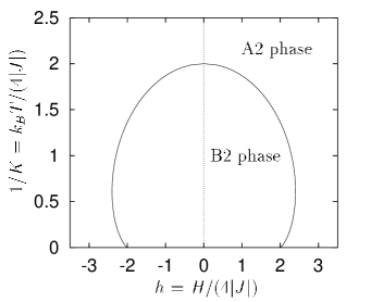
FIG. 2.: MF phase diagram of the NN Ising antiferromagnet on a bcc lattice, showing a line of continuous transitions between the disordered (A2) and the ordered (B2) phase.

The bulk sublattice magnetization densities may be written

$$m_{\alpha}=m+\phi\,,\quad m_{\beta}=m-\phi\,,$$ (21)

where $m$ and $\phi$ are the mean magnetization and the OP, respectively. In the region of the phase diagram where the A2 phase is thermodynamically stable, the bulk MF equations have a unique solution (see Appendix A)

$$m=m_{\text{dis}}(K,h)\,,\quad\phi=0\,.$$ (22)

Thus the only fixed points of $F^{2}$ and $G$ in this case are

$$\begin{array}[]{r@{\;=\;}l}\displaystyle\mathchoice{{\hbox{\boldmath$\displaystyle v$}}}{{\hbox{\boldmath$\textstyle v$}}}{{\hbox{\boldmath$\scriptstyle v$}}}{{\hbox{\boldmath$\scriptscriptstyle v$}}}_{\text{dis}}&\displaystyle(m_{\text{dis}},m_{\text{dis}})^{T}\,,\\ \displaystyle\mathchoice{{\hbox{\boldmath$\displaystyle w$}}}{{\hbox{\boldmath$\textstyle w$}}}{{\hbox{\boldmath$\scriptstyle w$}}}{{\hbox{\boldmath$\scriptscriptstyle w$}}}_{\text{dis}}&\displaystyle(m_{\text{dis}},m_{\text{dis}},m_{\text{dis}},m_{\text{dis}})^{T}\,.\end{array}$$ (23)

The solution (22) becomes thermodynamically unstable on crossing the critical line (Fig. 2). At the same time, two new solutions describing the pure B2 phases emerge,

$$m=m_{\text{ord}}(K,h)\,,\quad\phi=\pm\phi_{b}(K,h)\neq 0\,,$$ (24)

corresponding to the fixed points

$$\begin{array}[]{r@{\;=\;}l}\displaystyle\mathchoice{{\hbox{\boldmath$\displaystyle v$}}}{{\hbox{\boldmath$\textstyle v$}}}{{\hbox{\boldmath$\scriptstyle v$}}}{{\hbox{\boldmath$\scriptscriptstyle v$}}}_{\text{ord}}^{1,2}&\displaystyle(m_{\text{ord}}\mp\phi_{b},m_{\text{ord}}\pm\phi_{b})^{T}\,,\\ \displaystyle\mathchoice{{\hbox{\boldmath$\displaystyle w$}}}{{\hbox{\boldmath$\textstyle w$}}}{{\hbox{\boldmath$\scriptstyle w$}}}{{\hbox{\boldmath$\scriptscriptstyle w$}}}_{\text{ord}}^{1,2}&\displaystyle(m_{\text{ord}}\pm\phi_{b},m_{\text{ord}}\mp\phi_{b},m_{\text{ord}}\pm\phi_{b},m_{\text{ord}}\mp\phi_{b})^{T}\,.\end{array}$$ (25)

Note that the fixed points $\mathchoice{{\hbox{\boldmath$\displaystyle v$}}}{{\hbox{\boldmath$\textstyle v$}}}{{\hbox{\boldmath$\scriptstyle v$}}}{{\hbox{\boldmath$\scriptscriptstyle v$}}}_{\text{ord}}^{1}$, $\mathchoice{{\hbox{\boldmath$\displaystyle v$}}}{{\hbox{\boldmath$\textstyle v$}}}{{\hbox{\boldmath$\scriptstyle v$}}}{{\hbox{\boldmath$\scriptscriptstyle v$}}}_{\text{ord}}^{2}$ form a 2-cycle of the map $F$,

$$F\left(\mathchoice{{\hbox{\boldmath$\displaystyle v$}}}{{\hbox{\boldmath$\textstyle v$}}}{{\hbox{\boldmath$\scriptstyle v$}}}{{\hbox{\boldmath$\scriptscriptstyle v$}}}_{\text{ord}}^{1}\right)=\mathchoice{{\hbox{\boldmath$\displaystyle v$}}}{{\hbox{\boldmath$\textstyle v$}}}{{\hbox{\boldmath$\scriptstyle v$}}}{{\hbox{\boldmath$\scriptscriptstyle v$}}}_{\text{ord}}^{2}\,,\quad F\left(\mathchoice{{\hbox{\boldmath$\displaystyle v$}}}{{\hbox{\boldmath$\textstyle v$}}}{{\hbox{\boldmath$\scriptstyle v$}}}{{\hbox{\boldmath$\scriptscriptstyle v$}}}_{\text{ord}}^{2}\right)=\mathchoice{{\hbox{\boldmath$\displaystyle v$}}}{{\hbox{\boldmath$\textstyle v$}}}{{\hbox{\boldmath$\scriptstyle v$}}}{{\hbox{\boldmath$\scriptscriptstyle v$}}}_{\text{ord}}^{1}\,.$$ (26)

The bulk OP and the mean magnetization density at fixed bulk field $h=1$ are shown in Fig. 3 as a function of the reduced temperature

$\displaystyle t\equiv\frac{T-T_{c}}{T_{c}}=\frac{K_{c}-K}{K}\,.$The OP vanishes as $|t|^{\beta}$ for $t\to 0-$, with the usual MF exponent $\beta=1/2$ [Eq. (A10)]. The mean magnetization density is a nonordering (or noncritical) density. Typically, such quantities display $|t|^{1-\alpha}$ singularities, where $\alpha$ is the bulk specific heat exponent. In MF theory this behavior reduces to a discontinuity in the first temperature derivative since $\alpha=0$ [see Eqs. (A8) and (A10)].

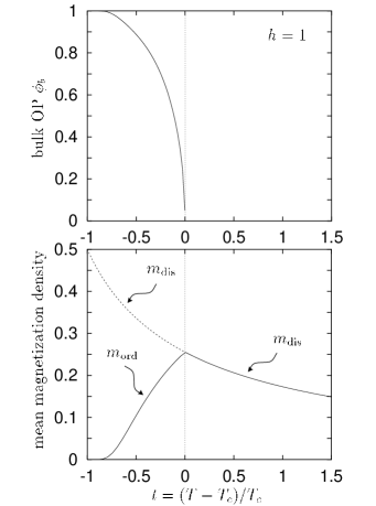
FIG. 3.: Temperature dependence of the bulk OP and mean magnetization density. Below $T_{c}$, the disordered state (dashed line) becomes thermodynamically unstable.

The linearization of $F^{2}$ about any of the fixed points $\mathchoice{{\hbox{\boldmath$\displaystyle v$}}}{{\hbox{\boldmath$\textstyle v$}}}{{\hbox{\boldmath$\scriptstyle v$}}}{{\hbox{\boldmath$\scriptscriptstyle v$}}}_{\text{dis}}$ and $\mathchoice{{\hbox{\boldmath$\displaystyle v$}}}{{\hbox{\boldmath$\textstyle v$}}}{{\hbox{\boldmath$\scriptstyle v$}}}{{\hbox{\boldmath$\scriptscriptstyle v$}}}_{\text{ord}}^{1,2}$ has the eigenvalues

$$\lambda_{1,2}=-1+2u_{\alpha}u_{\beta}\pm 2\sqrt{u_{\alpha}u_{\beta}}\sqrt{u_{\alpha}u_{\beta}-1}$$ (27)

and the associated eigenvectors

$$\mathchoice{{\hbox{\boldmath$\displaystyle l$}}}{{\hbox{\boldmath$\textstyle l$}}}{{\hbox{\boldmath$\scriptstyle l$}}}{{\hbox{\boldmath$\scriptscriptstyle l$}}}_{1,2}=\left(1,\,-\frac{1+\lambda_{1,2}}{2u_{\beta}}\right)^{T}\,,$$ (28)

where $u_{\alpha}$ and $u_{\beta}$ are defined by (A4). Since $F$ is symplectic and thus area-preserving (Sec. II), one has $\lambda_{1}\lambda_{2}=1$. Likewise, the eigenvalues of the linearization of $G$ about $\mathchoice{{\hbox{\boldmath$\displaystyle w$}}}{{\hbox{\boldmath$\textstyle w$}}}{{\hbox{\boldmath$\scriptstyle w$}}}{{\hbox{\boldmath$\scriptscriptstyle w$}}}_{\text{dis}}$ or $\mathchoice{{\hbox{\boldmath$\displaystyle w$}}}{{\hbox{\boldmath$\textstyle w$}}}{{\hbox{\boldmath$\scriptstyle w$}}}{{\hbox{\boldmath$\scriptscriptstyle w$}}}_{\text{ord}}^{1,2}$ are

$$\begin{array}[]{r@{\;=\;}l}\displaystyle\Lambda_{1,2}&\displaystyle-1+2\sqrt{u_{\alpha}u_{\beta}}\pm 2\sqrt{u_{\alpha}u_{\beta}-\sqrt{u_{\alpha}u_{\beta}}}\,,\\ \displaystyle\Lambda_{3,4}&\displaystyle-1-2\sqrt{u_{\alpha}u_{\beta}}\pm 2\sqrt{u_{\alpha}u_{\beta}+\sqrt{u_{\alpha}u_{\beta}}}\,,\end{array}$$ (29)

with the corresponding eigenvectors

$$\begin{array}[]{r@{\;=\;}r@{,\,}r@{,\,}r@{,\,}r}\displaystyle\mathchoice{{\hbox{\boldmath$\displaystyle L$}}}{{\hbox{\boldmath$\textstyle L$}}}{{\hbox{\boldmath$\scriptstyle L$}}}{{\hbox{\boldmath$\scriptscriptstyle L$}}}_{1,2}&\displaystyle\bigg{(}1&\displaystyle-\sqrt{\frac{u_{\alpha}}{u_{\beta}}}&\displaystyle\Lambda_{1,2}&\displaystyle-\sqrt{\frac{u_{\alpha}}{u_{\beta}}}\Lambda_{1,2}\bigg{)}^{T}\,,\\ \displaystyle\mathchoice{{\hbox{\boldmath$\displaystyle L$}}}{{\hbox{\boldmath$\textstyle L$}}}{{\hbox{\boldmath$\scriptstyle L$}}}{{\hbox{\boldmath$\scriptscriptstyle L$}}}_{3,4}&\displaystyle\bigg{(}1&\displaystyle\sqrt{\frac{u_{\alpha}}{u_{\beta}}}&\displaystyle\Lambda_{3,4}&\displaystyle\sqrt{\frac{u_{\alpha}}{u_{\beta}}}\Lambda_{3,4}\bigg{)}^{T}\,.\end{array}$$ (30)

Since $G$ is symplectic, the eigenvalues come in pairs ($\Lambda_{1}$, $\Lambda_{2}$) and ($\Lambda_{3}$, $\Lambda_{4}$) with $\Lambda_{1}\Lambda_{2}=\Lambda_{3}\Lambda_{4}=1$. Repeated application of the linearized map to $\mathchoice{{\hbox{\boldmath$\displaystyle L$}}}{{\hbox{\boldmath$\textstyle L$}}}{{\hbox{\boldmath$\scriptstyle L$}}}{{\hbox{\boldmath$\scriptscriptstyle L$}}}_{1,2}$ generates eigensolutions with opposite sublattice magnetization densities within each layer. Therefore, $\mathchoice{{\hbox{\boldmath$\displaystyle L$}}}{{\hbox{\boldmath$\textstyle L$}}}{{\hbox{\boldmath$\scriptstyle L$}}}{{\hbox{\boldmath$\scriptscriptstyle L$}}}_{1,2}$ represent “ordering” eigenmodes. The eigensolutions generated by $\mathchoice{{\hbox{\boldmath$\displaystyle L$}}}{{\hbox{\boldmath$\textstyle L$}}}{{\hbox{\boldmath$\scriptstyle L$}}}{{\hbox{\boldmath$\scriptscriptstyle L$}}}_{3,4}$ show an oscillating profile of the magnetization density because $\Lambda_{3,4}<0$. However, the local magnetization is the same for all sites in a given lattice plane parallel to the surface. Hence the OP profile vanishes and one may refer to $\mathchoice{{\hbox{\boldmath$\displaystyle L$}}}{{\hbox{\boldmath$\textstyle L$}}}{{\hbox{\boldmath$\scriptstyle L$}}}{{\hbox{\boldmath$\scriptscriptstyle L$}}}_{3,4}$ as “nonordering” eigenmodes.

FIG. 4.: Behavior of the eigenvalues (27) and (29) in the complex plane as one crosses the critical line (cf. Fig. 2). The superscripts “dis” and “ord” indicate the linearizations about the fixed points (23) and (25), respectively.

The behavior of the eigenvalues in the complex plane as one crosses the critical line is shown schematically in Fig. 4. The eigenvalues $\lambda_{1}$, $\lambda_{2}$ collide at $+1$ and form a complex conjugate pair on the unit circle in the ordered phase. Thus the character of the fixed point $\mathchoice{{\hbox{\boldmath$\displaystyle v$}}}{{\hbox{\boldmath$\textstyle v$}}}{{\hbox{\boldmath$\scriptstyle v$}}}{{\hbox{\boldmath$\scriptscriptstyle v$}}}_{\text{dis}}$ changes from hyperbolic to elliptic. At the same time, two new real eigenvalues corresponding to the hyperbolic fixed points $\mathchoice{{\hbox{\boldmath$\displaystyle v$}}}{{\hbox{\boldmath$\textstyle v$}}}{{\hbox{\boldmath$\scriptstyle v$}}}{{\hbox{\boldmath$\scriptscriptstyle v$}}}_{\text{ord}}^{1,2}$ emerge. Within the notions of nonlinear dynamics, the map $F$ undergoes a period-doubling bifurcation. The eigenvalues $\Lambda_{1}$, $\Lambda_{2}$ of the 4D map $G$ show an analogous behavior. However, the fixed point $\mathchoice{{\hbox{\boldmath$\displaystyle w$}}}{{\hbox{\boldmath$\textstyle w$}}}{{\hbox{\boldmath$\scriptstyle w$}}}{{\hbox{\boldmath$\scriptscriptstyle w$}}}_{\text{dis}}$ remains unstable in the ordered phase since $\Lambda_{3}$, $\Lambda_{4}$ stay real.

The solutions of the linearized MF equations satisfying the bulk boundary conditions (18) read

$$\mathchoice{{\hbox{\boldmath$\displaystyle v$}}}{{\hbox{\boldmath$\textstyle v$}}}{{\hbox{\boldmath$\scriptstyle v$}}}{{\hbox{\boldmath$\scriptscriptstyle v$}}}_{2n+1} = \mathchoice{{\hbox{\boldmath$\displaystyle v$}}}{{\hbox{\boldmath$\textstyle v$}}}{{\hbox{\boldmath$\scriptstyle v$}}}{{\hbox{\boldmath$\scriptscriptstyle v$}}}_{\ast}+a_{2}\lambda_{2}^{n}\mathchoice{{\hbox{\boldmath$\displaystyle l$}}}{{\hbox{\boldmath$\textstyle l$}}}{{\hbox{\boldmath$\scriptstyle l$}}}{{\hbox{\boldmath$\scriptscriptstyle l$}}}_{2}\,,$$

$$\mathchoice{{\hbox{\boldmath$\displaystyle w$}}}{{\hbox{\boldmath$\textstyle w$}}}{{\hbox{\boldmath$\scriptstyle w$}}}{{\hbox{\boldmath$\scriptscriptstyle w$}}}_{n+1} = \mathchoice{{\hbox{\boldmath$\displaystyle w$}}}{{\hbox{\boldmath$\textstyle w$}}}{{\hbox{\boldmath$\scriptstyle w$}}}{{\hbox{\boldmath$\scriptscriptstyle w$}}}_{\ast}+A_{2}\Lambda_{2}^{n}\mathchoice{{\hbox{\boldmath$\displaystyle L$}}}{{\hbox{\boldmath$\textstyle L$}}}{{\hbox{\boldmath$\scriptstyle L$}}}{{\hbox{\boldmath$\scriptscriptstyle L$}}}_{2}+A_{3}\Lambda_{3}^{n}\mathchoice{{\hbox{\boldmath$\displaystyle L$}}}{{\hbox{\boldmath$\textstyle L$}}}{{\hbox{\boldmath$\scriptstyle L$}}}{{\hbox{\boldmath$\scriptscriptstyle L$}}}_{3}\,,$$

where $\mathchoice{{\hbox{\boldmath$\displaystyle v$}}}{{\hbox{\boldmath$\textstyle v$}}}{{\hbox{\boldmath$\scriptstyle v$}}}{{\hbox{\boldmath$\scriptscriptstyle v$}}}_{\ast}$ and $\mathchoice{{\hbox{\boldmath$\displaystyle w$}}}{{\hbox{\boldmath$\textstyle w$}}}{{\hbox{\boldmath$\scriptstyle w$}}}{{\hbox{\boldmath$\scriptscriptstyle w$}}}_{\ast}$ stand for one of the fixed points (23) and (25). The coefficients $a_{2}$, $A_{2}$, and $A_{3}$ are fixed by the surface boundary conditions (16) and (17).

Thus for the (100) orientation we obtain

$$\begin{array}[]{r@{\;=\;}l}\displaystyle m_{2n+1}&\displaystyle m_{\alpha}+a\text{e}^{-(2n+1)/\xi}\,,\\ \displaystyle m_{2n}&\displaystyle m_{\beta}-b\text{e}^{-2n/\xi}\,,\end{array}$$ (31)

with the decay length

$$\xi=2\left|\ln\lambda_{2}\right|^{-1}\,,$$ (32)

and the amplitudes

$$a=(h_{1}+m_{\beta})\sqrt{\frac{u_{\beta}}{u_{\alpha}}}\,,\quad b=h_{1}+m_{\beta}\,.$$ (33)

In the disordered phase, the amplitudes simplify to

$$a=b=h_{1}+m_{\text{dis}}\,.$$ (34)

We define the local OP $\phi_{n}$ by

$$\phi_{n}\equiv{1\over 2}(-1)^{n}\left(m_{n+1}-m_{n}\right)\,,$$ (35)

where the power of $-1$ ensures that one always subtracts the magnetization densities of $\beta$-planes from those of $\alpha$-planes.[16] Eqs. (31) imply a nonvanishing OP profile, which decays on the scale of $\xi$. In fact, $\xi$ may be identified, up to a proportionality factor, with the bulk OP correlation length. To see this, one expands $u_{\alpha}u_{\beta}$ in Eq. (27) in powers of $t$ using (A8) and (A10). This gives

$$\xi=\xi_{\pm}|t|^{-1/2}+{\cal O}(t)\,,$$ (36)

where

$$\xi_{+} = \xi_{+}(h)=\frac{1}{2\sqrt{2-2K_{c}(h)m_{c}(h)[h-2m_{c}(h)]}}\,,$$ ()

$$\xi_{-} = \xi_{-}(h)=\frac{1}{\sqrt{2}}\xi_{+}(h)\,.$$ ()

The decay length displays a $|t|^{-\nu}$ singularity just as the bulk correlation length, with the MF exponent $\nu=1/2$. Asymptotically, $\xi$ should thus be proportional to the correlation length. Indeed, one has $\xi_{+}(h)/\xi_{-}(h)=\sqrt{2}$, which is the MF value of the universal amplitude ratio of the correlation lengths above and below $T_{c}$.[17] As $t\to 0$, the exponential decay of the OP profile becomes a power law, whose precise form will be investigated in Sec. IV.

Likewise, the magnetization profiles for the (110) orientation are

$$\begin{array}[]{r@{\;=\;}l}\displaystyle m_{n,\alpha}&\displaystyle m_{\alpha}+A\text{e}^{-n/\xi^{\prime}}+(-1)^{n}\tilde{A}\text{e}^{-n/\tilde{\xi}}\,,\\ \displaystyle m_{n,\beta}&\displaystyle m_{\beta}-B\text{e}^{-n/\xi^{\prime}}+(-1)^{n}\tilde{B}\text{e}^{-n/\tilde{\xi}},\end{array}$$ (37)

where now two length scales appear,

$$\xi^{\prime}=\left|\ln\Lambda_{2}\right|^{-1}\,,\quad\tilde{\xi}=\left|\ln\left|\Lambda_{3}\right|\right|^{-1}\,.$$ (38)

The amplitudes are given by

$$\begin{array}[]{r@{\;=\;}l}\displaystyle A&\displaystyle-\left(1-\sqrt{\frac{u_{\beta}}{u_{\alpha}}}\right)h_{1}-\frac{1}{2}\left(m_{\alpha}-\sqrt{\frac{u_{\beta}}{u_{\alpha}}}m_{\beta}\right)\,,\\ \displaystyle\tilde{A}&\displaystyle-\left(1+\sqrt{\frac{u_{\beta}}{u_{\alpha}}}\right)h_{1}-\frac{1}{2}\left(m_{\alpha}+\sqrt{\frac{u_{\beta}}{u_{\alpha}}}m_{\beta}\right)\,,\\ \displaystyle B&\displaystyle\sqrt{\frac{u_{\alpha}}{u_{\beta}}}A\,,\quad\tilde{B}=\sqrt{\frac{u_{\alpha}}{u_{\beta}}}\tilde{A}\,.\end{array}$$ (39)

In the disordered phase above $T_{c}$, they simplify to

$$A=B=0\,,\quad\tilde{A}=\tilde{B}=-2h_{1}-m_{\text{dis}}\,.$$ (40)

In particular, the OP profile

$$\phi_{n}\equiv\frac{1}{2}(m_{n,\alpha}-m_{n,\beta})$$ (41)

vanishes for $T\geq T_{c}$, which is a consequence of the symmetry of the (110) surface with respect to the two sublattices and the fact that neither enhanced surface couplings nor a staggered surface field are present. Asymptotically, $\xi^{\prime}$ and $\tilde{\xi}$ behave as

$$\xi^{\prime} = \frac{1}{\sqrt{2}}\xi_{\pm}|t|^{-1/2}+{\cal O}(t)\,,$$ ()

$$\tilde{\xi} = \left|\ln\left(3-2\sqrt{2}\right)\right|^{-1}+{\cal O}(t)\,,$$ ()

with $\xi_{\pm}$ given in (36) and $\left|\ln\left(3-2\sqrt{2}\right)\right|^{-1}\simeq 0.57$. The length $\xi^{\prime}$ associated with the ordering eigenmodes diverges as $t\to 0$ and may again be identified with the bulk correlation length (up to a proportionality constant),[18] whereas $\tilde{\xi}$ stays on the order of the lattice constant. As will be seen in the next section, $\tilde{\xi}$ describes the decay of the mean magnetization profile for $T\geq T_{c}$.

Note that for both surface orientations the layer magnetizations oscillate about $m_{\text{dis}}$ for $T>T_{c}$ due to the antiferromagnetic coupling between adjacent lattice planes. However, only in the case of the (100) orientation does this oscillating profile lead to a nonvanishing OP profile whose characteristic length scale diverges as $t\to 0+$. In view of the presumed absence of enhanced surface couplings, such a behavior should be due to an “effective” ordering surface field $g_{1}=g_{1}(K,h,h_{1})$. Away from $T_{c}$ and in the disordered phase, such a field generates a linear response of the local OP which decays exponentially into the bulk. A glance at (31) leads us to anticipate the form

$\displaystyle g_{1}(K,h,h_{1})=h_{1}+m_{\text{dis}}(K,h)\,.$We will derive a formula for $g_{1}$ identical with the above expression in Sec. IV, when we map the lattice model onto a continuum theory. There it will become clear that $g_{1}$ is indeed a surface field coupling to the local OP that enters into a coarse-grained (Ginzburg-Landau) free-energy functional.

B Solutions of the nonlinear recursive maps

The thermodynamically stable solutions of the bulk MF equations correspond to hyperbolic fixed points of the maps $F^{2}$ and $G$ (cf. Sec. III A). The stable (unstable) manifold $W_{s}$ ($W_{u}$), or inset (outset), of a hyperbolic fixed point consists of all points that converge to the fixed point under iteration of the map (inverse map). In order to solve the MF equations for the semi-infinite system one must determine the intersections of the stable manifolds with the linear subspaces defined by the surface boundary conditions (16) and (17), i. e., the line $\left\{(-h_{1},x)^{T}\big{|}\,x\in{\mathbb{R}}\right\}$ and the hyperplane $\left\{(-2h_{1},-2h_{1},x,y)^{T}\big{|}\,x,y\in{\mathbb{R}}\right\}$. The magnetization densities of the first layer can be read off from the intersection points $\mathchoice{{\hbox{\boldmath$\displaystyle v$}}}{{\hbox{\boldmath$\textstyle v$}}}{{\hbox{\boldmath$\scriptstyle v$}}}{{\hbox{\boldmath$\scriptscriptstyle v$}}}_{1}=(-h_{1},m_{1})^{T}$ and $\mathchoice{{\hbox{\boldmath$\displaystyle w$}}}{{\hbox{\boldmath$\textstyle w$}}}{{\hbox{\boldmath$\scriptstyle w$}}}{{\hbox{\boldmath$\scriptscriptstyle w$}}}_{1}=(-2h_{1},-2h_{1},m_{1,\alpha},m_{1,\beta})^{T}$. The complete magnetization profile follows from the trajectories passing through $\mathchoice{{\hbox{\boldmath$\displaystyle v$}}}{{\hbox{\boldmath$\textstyle v$}}}{{\hbox{\boldmath$\scriptstyle v$}}}{{\hbox{\boldmath$\scriptscriptstyle v$}}}_{1}$ and $\mathchoice{{\hbox{\boldmath$\displaystyle w$}}}{{\hbox{\boldmath$\textstyle w$}}}{{\hbox{\boldmath$\scriptstyle w$}}}{{\hbox{\boldmath$\scriptscriptstyle w$}}}_{1}$.[19] Below $T_{c}$, infinitely many intersections exist and one has to resort to the original variational principle to find the equilibrium profile minimizing the free-energy functional (6).

1 (100) surface, $T\geq T_{c}$

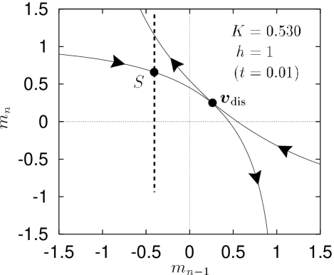
FIG. 5.: Invariant manifolds (inset and outset) of the hyperbolic fixed point $\mathchoice{{\hbox{\boldmath$\displaystyle v$}}}{{\hbox{\boldmath$\textstyle v$}}}{{\hbox{\boldmath$\scriptstyle v$}}}{{\hbox{\boldmath$\scriptscriptstyle v$}}}_{\text{dis}}$. The direction of the flow under iteration of the map $F$ is indicated by arrows. The dashed line represents the boundary condition for $h_{1}=0.4$.

In the disordered phase, the only fixed point of $F^{2}$ (as well as of $F$) is $\mathchoice{{\hbox{\boldmath$\displaystyle v$}}}{{\hbox{\boldmath$\textstyle v$}}}{{\hbox{\boldmath$\scriptstyle v$}}}{{\hbox{\boldmath$\scriptscriptstyle v$}}}_{\text{dis}}=(m_{\text{dis}},m_{\text{dis}})^{T}$ [Eq. (23)]. Fig. 5 shows a plot of the invariant manifolds for particular values of $K$ and $h$. Fig. 6 depicts the magnetization and OP profiles obtained from the intersection with the boundary condition for $h_{1}=0.4$. Since $R\circ F=F^{-1}\circ R$ [cf. Eq. (19)], the inset and outset are mapped onto each other under reflection at the line $x=y$.

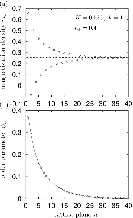
FIG. 6.: (a) Magnetization profile $m_{n}$ for the (100) surface above $T_{c}$, as obtained from the intersection $S$ of Fig. 5. Odd and even planes $n$ belong to sublattice $\alpha$ ($\Diamond$) and $\beta$ ($\times$), respectively. Note that $m_{n}$ oscillates about the bulk value $m_{\text{dis}}$ (dashed line). (b) OP profile, defined by (35). For convenience, the discrete points have been joined by lines.

The picture of the invariant manifolds does not change qualitatively as one varies the parameters $K$ and $h$. From the eigenvector $\mathchoice{{\hbox{\boldmath$\displaystyle l$}}}{{\hbox{\boldmath$\textstyle l$}}}{{\hbox{\boldmath$\scriptstyle l$}}}{{\hbox{\boldmath$\scriptscriptstyle l$}}}_{2}$ [Eq. (28)] one infers that the slope of the inset at $\mathchoice{{\hbox{\boldmath$\displaystyle v$}}}{{\hbox{\boldmath$\textstyle v$}}}{{\hbox{\boldmath$\scriptstyle v$}}}{{\hbox{\boldmath$\scriptscriptstyle v$}}}_{\text{dis}}$ vanishes in the high-temperature limit ($K\to 0$), whereas it approaches $-1$ for $K\uparrow K_{c}$ ($T\downarrow T_{c}$).

The upshot is that we find a unique intersection of the boundary condition with the stable manifold. In particular, we obtain a nonvanishing order parameter profile at any temperature $T>T_{c}$. This conforms with the idea that the OP profile is due to an ordering surface field.

An exceptional case occurs if the boundary condition exactly hits the fixed point $\mathchoice{{\hbox{\boldmath$\displaystyle v$}}}{{\hbox{\boldmath$\textstyle v$}}}{{\hbox{\boldmath$\scriptstyle v$}}}{{\hbox{\boldmath$\scriptscriptstyle v$}}}_{\text{dis}}$, so that $m_{n}\equiv m_{\text{dis}}$ and $\phi_{n}\equiv 0$. However, except in the case $h=h_{1}=0$, this can only be achieved for a special temperature $T=T_{0}$ (at fixed $h$ and $h_{1}$). For $T\neq T_{0}$ the OP profile is still nonzero.

2 (110) surface, $T\geq T_{c}$

As we have seen in Sec. I, this type of surface is symmetry-preserving and the Hamiltonian (4) is exactly symmetric with respect to interchanging $\alpha$ and $\beta$-sites. Since we precluded the possibility of supercritically enhanced surface bonds, a spontaneous breakdown of this symmetry is ruled out for $T\geq T_{c}$. Therefore the solutions that minimize the free energy in this temperature regime fulfill $m_{n,\alpha}=m_{n,\beta}\equiv m_{n}$, and $G$ acts in a 2D subset $\left\{(x,x,y,y)^{T}\big{|}\,x\in{\mathbb{R}}\,,\;|y|<1\right\}$ of ${\mathbb{R}}^{4}$. The picture of the invariant manifolds looks similar to Fig. 5. The magnetization profile at the bulk critical point $K=K_{c}(h)$ (for $h=1$) is depicted in Fig. 7. As in the case of the (100) orientation, the layer magnetization densities oscillate about the bulk value $m_{\text{dis}}$ due to the antiferromagnetic coupling between neighboring planes. However, the decay length remains on the order of the lattice constant even at $T=T_{c}$, (cf. Sec. III A). The numerical profile decays exponentially on a length scale that agrees well with the value (() ‣ III A).

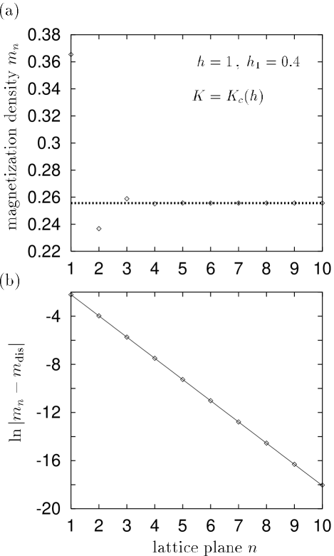
FIG. 7.: (a) Magnetization profile at $T=T_{c}$ for the (110) surface. The dashed line represents the bulk value $m_{\text{dis}}$. (b) Exponential decay of the profile. The solid curve is a straight line with slope $\tilde{\xi}^{-1}$ [Eq. (() ‣ III A)].

3 (100) surface, $T<T_{c}$

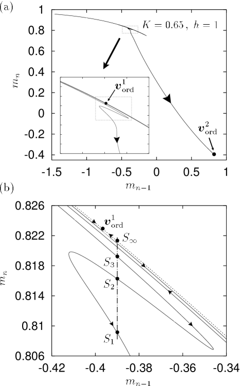
FIG. 8.: (a) Part of the stable manifold of the fixed point $\mathchoice{{\hbox{\boldmath$\displaystyle v$}}}{{\hbox{\boldmath$\textstyle v$}}}{{\hbox{\boldmath$\scriptstyle v$}}}{{\hbox{\boldmath$\scriptscriptstyle v$}}}_{\text{ord}}^{2}$. The inset shows the first few loops in the vicinity of $\mathchoice{{\hbox{\boldmath$\displaystyle v$}}}{{\hbox{\boldmath$\textstyle v$}}}{{\hbox{\boldmath$\scriptstyle v$}}}{{\hbox{\boldmath$\scriptscriptstyle v$}}}_{\text{ord}}^{1}$. (b) Magnification of the region marked in the inset of (a). The dashed-dotted line is the boundary condition for $h_{1}=0.39$, which intersects the stable manifold at an infinite number of points $S_{1}$, $S_{2}$, $\ldots$. The latter accumulate at the point $S_{\infty}$ on the stable manifold of $\mathchoice{{\hbox{\boldmath$\displaystyle v$}}}{{\hbox{\boldmath$\textstyle v$}}}{{\hbox{\boldmath$\scriptstyle v$}}}{{\hbox{\boldmath$\scriptscriptstyle v$}}}_{\text{ord}}^{1}$ (dashed line).

On crossing the critical line in the MF phase diagram (Fig. 2), the map $F$ undergoes a period-doubling bifurcation (Sec. III A), and the picture of the invariant manifolds changes qualitatively. The fixed point $\mathchoice{{\hbox{\boldmath$\displaystyle v$}}}{{\hbox{\boldmath$\textstyle v$}}}{{\hbox{\boldmath$\scriptstyle v$}}}{{\hbox{\boldmath$\scriptscriptstyle v$}}}_{\text{dis}}$ becomes elliptic and looses any inset and outset. The inset (outset) of any one of the hyperbolic fixed points $\mathchoice{{\hbox{\boldmath$\displaystyle v$}}}{{\hbox{\boldmath$\textstyle v$}}}{{\hbox{\boldmath$\scriptstyle v$}}}{{\hbox{\boldmath$\scriptscriptstyle v$}}}_{\text{ord}}^{1,2}$ cannot intersect itself but will generically intersect the outset (inset) of the same fixed point, as well as the outsets (insets) of all other fixed points, at an infinite number of so-called homoclinic and heteroclinic points.[13] The invariant manifolds oscillate wildly in the vicinity of the fixed points (cf. Fig. 8), giving rise to the phenomenon of “chaotic entanglement”.[13] As a consequence, infinitely many solutions of the lattice MF equations for the semi-infinite system exist, and one has to resort to the original variational principle (cf. Sec. II) in order to decide which solution corresponds to the true equilibrium profile. The stable and unstable manifolds $W_{s}$ and $W_{u}$ of $\mathchoice{{\hbox{\boldmath$\displaystyle v$}}}{{\hbox{\boldmath$\textstyle v$}}}{{\hbox{\boldmath$\scriptstyle v$}}}{{\hbox{\boldmath$\scriptscriptstyle v$}}}_{\text{ord}}^{1}$ and $\mathchoice{{\hbox{\boldmath$\displaystyle v$}}}{{\hbox{\boldmath$\textstyle v$}}}{{\hbox{\boldmath$\scriptstyle v$}}}{{\hbox{\boldmath$\scriptscriptstyle v$}}}_{\text{ord}}^{2}$ are determined uniquely given only one of them, say $W_{s}\!\left(\mathchoice{{\hbox{\boldmath$\displaystyle v$}}}{{\hbox{\boldmath$\textstyle v$}}}{{\hbox{\boldmath$\scriptstyle v$}}}{{\hbox{\boldmath$\scriptscriptstyle v$}}}_{\text{ord}}^{1}\right)$. In fact, from the symmetry property (19) one concludes that

$$W_{u}\left(\mathchoice{{\hbox{\boldmath$\displaystyle v$}}}{{\hbox{\boldmath$\textstyle v$}}}{{\hbox{\boldmath$\scriptstyle v$}}}{{\hbox{\boldmath$\scriptscriptstyle v$}}}_{\text{ord}}^{1}\right) = F\circ R\biglb(W_{s}\!\left(\mathchoice{{\hbox{\boldmath$\displaystyle v$}}}{{\hbox{\boldmath$\textstyle v$}}}{{\hbox{\boldmath$\scriptstyle v$}}}{{\hbox{\boldmath$\scriptscriptstyle v$}}}_{\text{ord}}^{1}\right)\bigrb)\,,$$

$$W_{s}\left(\mathchoice{{\hbox{\boldmath$\displaystyle v$}}}{{\hbox{\boldmath$\textstyle v$}}}{{\hbox{\boldmath$\scriptstyle v$}}}{{\hbox{\boldmath$\scriptscriptstyle v$}}}_{\text{ord}}^{2}\right) = F\biglb(W_{s}\!\left(\mathchoice{{\hbox{\boldmath$\displaystyle v$}}}{{\hbox{\boldmath$\textstyle v$}}}{{\hbox{\boldmath$\scriptstyle v$}}}{{\hbox{\boldmath$\scriptscriptstyle v$}}}_{\text{ord}}^{1}\right)\bigrb)\,,$$

$$W_{u}\left(\mathchoice{{\hbox{\boldmath$\displaystyle v$}}}{{\hbox{\boldmath$\textstyle v$}}}{{\hbox{\boldmath$\scriptstyle v$}}}{{\hbox{\boldmath$\scriptscriptstyle v$}}}_{\text{ord}}^{2}\right) = R\biglb(W_{s}\!\left(\mathchoice{{\hbox{\boldmath$\displaystyle v$}}}{{\hbox{\boldmath$\textstyle v$}}}{{\hbox{\boldmath$\scriptstyle v$}}}{{\hbox{\boldmath$\scriptscriptstyle v$}}}_{\text{ord}}^{1}\right)\bigrb)\,.$$

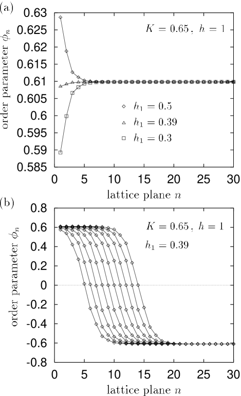
FIG. 9.: (a) OP profiles below $T_{c}$ for the (100) surface. The corresponding trajectories converge to the fixed point $\mathchoice{{\hbox{\boldmath$\displaystyle v$}}}{{\hbox{\boldmath$\textstyle v$}}}{{\hbox{\boldmath$\scriptstyle v$}}}{{\hbox{\boldmath$\scriptscriptstyle v$}}}_{\text{ord}}^{1}$ (cf. Fig. 8b). The middle profile ($h_{1}=0.39$) belongs to the intersection $S_{\infty}$. (b) OP profiles describing an antiphase boundary. The trajectories converge to $\mathchoice{{\hbox{\boldmath$\displaystyle v$}}}{{\hbox{\boldmath$\textstyle v$}}}{{\hbox{\boldmath$\scriptstyle v$}}}{{\hbox{\boldmath$\scriptscriptstyle v$}}}_{\text{ord}}^{2}$. The leftmost profile belongs to the intersection $S_{1}$, the next one to $S_{2}$, etc. (Fig. 8b). An infinite number of such solutions exists, the first ten of which are shown here.

Typical minimum-free-energy profiles are shown in Fig. 9a. The corresponding trajectories converge to the fixed point $\mathchoice{{\hbox{\boldmath$\displaystyle v$}}}{{\hbox{\boldmath$\textstyle v$}}}{{\hbox{\boldmath$\scriptstyle v$}}}{{\hbox{\boldmath$\scriptscriptstyle v$}}}_{1}$ describing the bulk phase $\phi_{b}>0$. If one imposes the bulk boundary condition $\phi_{n}\to-\phi_{b}<0$ ($n\to\infty$), so that the solutions converge to $\mathchoice{{\hbox{\boldmath$\displaystyle v$}}}{{\hbox{\boldmath$\textstyle v$}}}{{\hbox{\boldmath$\scriptstyle v$}}}{{\hbox{\boldmath$\scriptscriptstyle v$}}}_{2}$, one obtains OP profiles exhibiting an antiphase boundary, i. e., an interface between the two phases $\pm\phi_{b}$ (Fig. 9b). These solutions always yield a higher free energy than the profiles of Fig. 9a. For the chosen parameter values, the free energy of the profiles is found to increase as the position of the interface moves into the bulk, so that the leftmost profile represents the equilibrium solution for this type of boundary conditions. By analogy with wetting phenomena,[20] we may say that the surface is “nonwet”, i. e., the interface has a finite (microscopic) distance from the surface. If $h_{1}$ is increased, so that the “effective” ordering surface field $g_{1}$ favoring the bulk phase $\phi_{b}>0$ becomes strong enough, the free energy of the profiles eventually decreases and the surface is “wet”. (E. g., in the situation depicted in Fig. 9b this happens if one chooses $h_{1}=0.4$.) In Ref. [21] the wetting phase diagram in the space of thermodynamic parameters $K$, $h$, and $h_{1}$ is calculated using the continuum model derived in the next section.

IV Ginzburg-Landau theory

In this section, the aim is to derive and critically examine a Ginzburg-Landau model for the semi-infinite alloy with a (100) surface. In particular, we want to show that the loss of the $\alpha\leftrightarrow\beta$ sublattice symmetry (cf. Sec. I) leads, in a continuum description, to a symmetry-breaking boundary condition for the OP profile $\phi(z)$,

$\displaystyle\dot{\phi}(0)=\frac{1}{\lambda}\phi(0)-\frac{g_{1}}{C}\,,$where $z=0$ corresponds to the surface plane ($n=1$) and the dot denotes differentiation with respect to $z$. Such a boundary condition is familiar from the phenomenological theory of surface critical phenomena.[3] The parameter $C>0$ is the coefficient of the gradient term of the Ginzburg-Landau functional. The extrapolation length $\lambda$ should be positive owing to the absence of enhanced surface bonds. Thus the persistence of surface order for $T\geq T_{c}$ originates solely from the “effective” ordering surface field $g_{1}\neq 0$. We will determine the dependence of $g_{1}=g_{1}(K,h,h_{1})$ on the reduced coupling constant $K$ and the fields $h$ and $h_{1}$.

No such ordering surface field emerges in the case of the symmetry-preserving (110) surface. However, the Ginzburg-Landau functional depends on an additional spatially varying nonordering density to which the surface field $h_{1}$ couples. We defer the derivation of the corresponding continuum model to a subsequent paper,[22] where nonordering densities and the construction of suitable multicomponent Ginzburg-Landau theories will be treated from a more general perspective.

Upon approaching the bulk critical point in the presence of an ordering surface field $g_{1}\neq 0$, the semi-infinite system undergoes the normal transition, which exhibits critical singularities that are distinct from those of the ordinary transition. The latter occurs for $g_{1}=0$ and subcritical surface enhancement ($\lambda>0$).[23] In order to confirm that the continuum theory derived in Sec. IV A correctly describes the asymptotic critical behavior of the lattice model, we shall draw a detailed numerical comparison with the solutions of the lattice MF equations and clearly identify the singular behavior of the normal transition for generic values of $h$ and $h_{1}$ (Sec. IV B). By tuning $h$ and $h_{1}$, one can achieve that $g_{1}=0$ at $T=T_{c}$. Then the singularities of the ordinary transition are recovered, although the OP at the surface is nonzero for $T>T_{c}$ because of $g_{1}\neq 0$ for $T\neq T_{c}$ (Sec. IV C).

A Derivation of continuum model

One has to be careful to define the local OP $\phi_{n}$ in such a way that the space-inversion symmetry of the lattice MF equations (8) survives the continuum limit. If the magnetization profile $m_{n}$, $n=1,2,\ldots$, is a solution of (8), so is the profile $\tilde{m}_{-n}\equiv m_{n+2}$ obtained by reflection at the surface plane $n=1$. If the definition of $\phi_{n}$ respects this symmetry, the differential equation for the continuum profile $\phi(z)$ should be invariant under $\phi(z)\to\phi(-z)$. However, the definition (35) distinguishes one direction along the [100] axis and violates space-inversion symmetry explicitly. As a consequence, first-order derivatives of $\phi(z)$ appear in the Ginzburg-Landau equations, corresponding to linear derivative terms in the free-energy functional.[6] Such terms render the functional unbounded from below and thus preclude it from serving as a Landau-Ginzburg-Wilson Hamiltonian of a field theory.

To avoid these difficulties, we adopt an alternate definition of the local OP treating the two neighboring layers of lattice plane $n$ on an equal footing:

$$\phi_{n}\equiv\frac{1}{2}(-1)^{n}\left[\frac{1}{2}(m_{n-1}+m_{n+1})-m_{n}\right]\,.$$ (43)

This definition complies with space-inversion symmetry and coincides with (35) in the bulk of the system.

Substituting $m_{n+1}+m_{n-1}$ from (8) into (43) we obtain

$$\phi_{n}=(-1)^{n+1}\varphi(m_{n})\,,$$ (44)

where the function

$\displaystyle\varphi(x)\equiv-\frac{h}{4}+\frac{x}{2}+\frac{1}{4K}\tanh^{-1}x$is strictly monotonous and thus invertible. We denote the inverse of $\varphi$ by ${\cal M}$, so that from (44)

$$m_{n}={\cal M}\biglb((-1)^{n+1}\phi_{n}\bigrb)\,.$$ (45)

The continuum limit of the lattice MF equations (8) leads to the Ginzburg-Landau equation (see Appendix B)

$$C\ddot{\phi}=4\phi+2{\cal M}(-\phi)-2{\cal M}(\phi)\,,$$ (46)

where $C\equiv{\cal M}^{\prime}(0)$ [Eq. (() ‣ B)]. The MF equation at the surface (9) entails the boundary condition (see Appendix C)

$$C\dot{\phi}(0)=-h_{1}-{\cal M}\mathchoice{{\hbox{\boldmath$\displaystyle($}}}{{\hbox{\boldmath$\textstyle($}}}{{\hbox{\boldmath$\scriptstyle($}}}{{\hbox{\boldmath$\scriptscriptstyle($}}}\!-\!\phi(0)\mathchoice{{\hbox{\boldmath$\displaystyle)$}}}{{\hbox{\boldmath$\textstyle)$}}}{{\hbox{\boldmath$\scriptstyle)$}}}{{\hbox{\boldmath$\scriptscriptstyle)$}}}\,.$$ (47)

For a spatially homogeneous system, (46) is identical to the equation for the OP following from the bulk MF equations (A3^′). In fact, (A3^′) can be written as

$\displaystyle\phi=\varphi(m+\phi)\,,\quad-\phi=\varphi(m-\phi)\,.$Operating with $\cal M$ on both sides of the above equations and eliminating $m$, one arrives at (46) with $\ddot{\phi}\equiv 0$.

We denote the bulk Landau free-energy density by $f_{b}(m_{\alpha},m_{\beta})$ [Eq. (A2)]. Since

$$\partial_{\alpha}f_{b}(m_{\alpha},m_{\beta}) = 2\varphi(m_{\alpha})-(m_{\alpha}-m_{\beta})\,,$$

$$\partial_{\beta}f_{b}(m_{\alpha},m_{\beta}) = 2\varphi(m_{\beta})+(m_{\alpha}-m_{\beta})\,,$$

where $\partial_{\mu}\equiv\frac{\partial}{\partial m_{\mu}}$, $\mu=\alpha,\beta$, Eqs. (46) and (47) can be rewritten as

$$C\ddot{\phi} = V^{\prime}(\phi)\,,$$ ()

$$C\dot{\phi}(0) = f_{s}^{\prime}(\phi)\,,$$ ()

where

$$V(\phi) = \frac{1}{2}[{\cal M}(\phi)-{\cal M}(-\phi)-2\phi]^{2}$$ (49)

$${}+f_{b}\mathchoice{{\hbox{\boldmath$\displaystyle($}}}{{\hbox{\boldmath$\textstyle($}}}{{\hbox{\boldmath$\scriptstyle($}}}{{\hbox{\boldmath$\scriptscriptstyle($}}}{\cal M}(\phi),{\cal M}(-\phi)\mathchoice{{\hbox{\boldmath$\displaystyle)$}}}{{\hbox{\boldmath$\textstyle)$}}}{{\hbox{\boldmath$\scriptstyle)$}}}{{\hbox{\boldmath$\scriptscriptstyle)$}}}-f_{b}\mathchoice{{\hbox{\boldmath$\displaystyle($}}}{{\hbox{\boldmath$\textstyle($}}}{{\hbox{\boldmath$\scriptstyle($}}}{{\hbox{\boldmath$\scriptscriptstyle($}}}{\cal M}(0),{\cal M}(0)\mathchoice{{\hbox{\boldmath$\displaystyle)$}}}{{\hbox{\boldmath$\textstyle)$}}}{{\hbox{\boldmath$\scriptstyle)$}}}{{\hbox{\boldmath$\scriptscriptstyle)$}}}\,,$$

$$f_{s}(\phi) = -[h_{1}+{\cal M}(-\phi)]\phi+\frac{1}{4}f_{b}\mathchoice{{\hbox{\boldmath$\displaystyle($}}}{{\hbox{\boldmath$\textstyle($}}}{{\hbox{\boldmath$\scriptstyle($}}}{{\hbox{\boldmath$\scriptscriptstyle($}}}{\cal M}(-\phi),{\cal M}(-\phi)\mathchoice{{\hbox{\boldmath$\displaystyle)$}}}{{\hbox{\boldmath$\textstyle)$}}}{{\hbox{\boldmath$\scriptstyle)$}}}{{\hbox{\boldmath$\scriptscriptstyle)$}}}\,.$$ (51)

$${}-\frac{1}{4}f_{b}\mathchoice{{\hbox{\boldmath$\displaystyle($}}}{{\hbox{\boldmath$\textstyle($}}}{{\hbox{\boldmath$\scriptstyle($}}}{{\hbox{\boldmath$\scriptscriptstyle($}}}{\cal M}(0),{\cal M}(0)\mathchoice{{\hbox{\boldmath$\displaystyle)$}}}{{\hbox{\boldmath$\textstyle)$}}}{{\hbox{\boldmath$\scriptstyle)$}}}{{\hbox{\boldmath$\scriptscriptstyle)$}}}\,.$$

Thus the Ginzburg-Landau equations (46) and (47) follow from the variation of the free-energy functional

$${\cal F}[\phi]=\int_{0}^{\infty}dz\,\left[\frac{C}{2}\dot{\phi}^{2}+V(\phi)\right]+f_{s}\mathchoice{{\hbox{\boldmath$\displaystyle($}}}{{\hbox{\boldmath$\textstyle($}}}{{\hbox{\boldmath$\scriptstyle($}}}{{\hbox{\boldmath$\scriptscriptstyle($}}}\phi(0)\mathchoice{{\hbox{\boldmath$\displaystyle)$}}}{{\hbox{\boldmath$\textstyle)$}}}{{\hbox{\boldmath$\scriptstyle)$}}}{{\hbox{\boldmath$\scriptscriptstyle)$}}}\,.$$ (52)

Expansion of $V(\phi)$ yields the usual $\phi^{4}$-form

$$V(\phi)=\frac{A}{2}\phi^{2}+\frac{B}{4}\phi^{4}+{\cal O}\left(\phi^{6}\right)\,,$$ (53)

where $A=4(1-M_{1})$ and $B=-4M_{3}$ [Eqs. (() ‣ B)]. With the aid of (A8), the leading temperature dependence of the Landau coefficients is found to be

$$A = A_{1}t+{\cal O}\left(t^{2}\right)\,,$$ ()

$$B = B_{0}+{\cal O}(t)\,,$$ ()

$$C = 1+{\cal O}(t)\,.$$ ()

where

$$A_{1} = A_{1}(h)=2\{1-K_{c}(h)m_{c}(h)[h-2m_{c}(h)]\}\,,$$

$$B_{0} = B_{0}(h)=\frac{8}{3}K_{c}(h)^{2}\,.$$

Likewise, the Landau expansion of $f_{s}(\phi)$ reads

$$f_{s}(\phi)=-g_{1}\phi+\frac{C}{2\lambda}\phi^{2}+{\cal O}\left(\phi^{3}\right)\,,$$ (54)

where

$$g_{1}(K,h,h_{1}) = h_{1}+m_{\text{dis}}(K,h)\,,$$ ()

$$\lambda = 1\,.$$ ()

Thus we obtain a positive extrapolation length $\lambda$ and an ordering surface field $g_{1}\neq 0$, as anticipated above.

B Comparison with lattice MF theory: generic (nonideal) stoichiometry

If $h$ and $h_{1}$ take generic values (nonideal bulk and surface stoichiometry), $g_{1}=g_{1}(K,h,h_{1})$ is nonzero at $T=T_{c}$ and gives rise to an OP profile decaying according to a power law. For $t=0$, (46^′) becomes

$$\ddot{\phi}=B_{0}\phi^{3}\,.$$ (55)

The neglected higher powers of $\phi$ do not affect the asymptotic behavior of $\phi(z)$ as $z\to\infty$. The solution of (55) satisfying $\phi(z)\to 0$ as $z\to\infty$ reads

$$\phi(z)=\frac{P_{0}}{z+z_{0}}\,,$$ (56)

with the amplitude

$$P_{0}(h)=\pm\sqrt{\frac{2}{B_{0}(h)}}=\pm\frac{\sqrt{3}}{2K_{c}(h)}\,.$$ (57)

The signs refer to positive and negative $g_{1}$, respectively. The integration constant $z_{0}$ follows by inserting (55a) into the boundary condition (47). An algebraic decay $\phi(z)\sim z^{-x_{\phi}}$ of the OP profile at $T=T_{c}$, where $x_{\phi}$ is the scaling dimension of the OP, is characteristic of the normal transition. Generally, $x_{\phi}$ can be expressed by bulk critical exponents as $x_{\phi}=\beta/\nu$. Within MF theory, $\beta=\nu=1/2$, so that $x_{\phi}=1$.

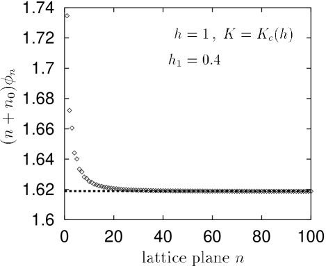
FIG. 10.: Scaling of the critical OP profile $\phi_{n}$ [defined by (43)]. The expected power law decay has been factored out. The parameter $n_{0}$ was fitted optimally. The dashed line is the prediction (55b) of the continuum theory.

In order to check whether the lattice MF profiles exhibit the above power law decay with the predicted value (55b) for the amplitude, we used the “nonlinear-mapping representation” of the lattice MF equations (Sec. III) to determine the profiles numerically up to $\simeq 1000$ layers from the surface. Fig. 10 demonstrates that the power law decay is well reproduced. The amplitude extracted from the numerical fits is in perfect agreement with (55b) for a wide range of the bulk field $h$ (Fig. 11).

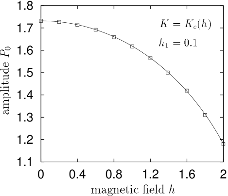
FIG. 11.: Amplitude of the critical OP profile as a function of the bulk field $h$. The data obtained from the solution of the lattice MF equations ($\Box$) agree well with the prediction (55b) of the continuum model (full line).

As a second test of the validity of our continuum model we investigate the temperature singularity of the surface OP. We multiply the Ginzburg-Landau equation (46^′) by $\dot{\phi}$ and perform the integral from $z=0$ to $z=\infty$ on both sides using the boundary conditions (47^′) and $\phi(z)\to 0$ as $z\to\infty$. This gives

$$-\frac{C}{2}f_{s}^{\prime}(\phi_{s})^{2}+V(\phi_{s})=V_{\infty}\,,$$ (58)

where $\phi_{s}\equiv\phi(0)$ and $V_{\infty}\equiv V(\phi_{b})$. One has

$\displaystyle V_{\infty}=\left\{\begin{array}[]{lr}0\,,&t>0\,,\\ -\frac{A_{1}^{2}}{2B_{0}}t^{2}+{\cal O}\left(t^{3}\right)\,,&t<0\,.\end{array}\right.$Expanding the coefficients on both sides of the surface equation of state (58) in powers of $t$, one recognizes that $\phi_{s}$ exhibits a discontinuity in the second temperature derivative due to the non-analyticity of $V_{\infty}$ at $t=0$,

$$\phi_{s}=\phi_{s}^{(0)}+\phi_{s}^{(1)}t+\phi_{s,\pm}^{(2)}t^{2}+\ldots\,,$$ (59)

with $\phi_{s,+}^{(2)}\neq\phi_{s,-}^{(2)}$. This result complies with the general form of the leading $|t|^{2-\alpha}$ singularity of the surface OP at the normal and extraordinary transitions.[24]

FIG. 12.: Temperature dependence of the surface OP $\phi_{s}$ for generic values of $h$, $h_{1}$, in the immediate vicinity of the critical temperature. The results of the lattice MF theory ($\Box$) agree well with the prediction of the continuum model (solid line).

Fig. 12 shows a comparison with the solutions of the lattice MF equations. While the singularity in the second temperature derivative is too weak to be detected without considerable numerical effort, the data are fully consistent with the continuity of the first temperature derivative at $t=0$ and agree well with the predictions of the continuum theory. The continuity of the first temperature derivative of $\phi_{s}$ is incompatible with the ordinary transition and confirms again that the asymptotic critical behavior falls into the universality class of the normal transition.

C Comparison with lattice MF theory: Vanishing ordering surface field at $T=T_{c}$

According to (54a), $g_{1}$ can be made to vanish at $T=T_{c}$ by choosing $h_{1}$ such that

$$h_{1}=-m_{c}(h)\,.$$ (60)

If $h=h_{1}=0$ (ideal bulk and surface stoichiometry), $g_{1}\equiv 0$ for all temperatures, and the system clearly displays ordinary surface critical behavior. If $h\neq 0$ and (60) is fulfilled, $g_{1}$ varies linearly with $t$ as $t\to 0$. In particular, the surface OP $\phi_{s}$ is nonzero for $T>T_{c}$ and vanishes only in the limit $t\to 0\pm$. One may wonder whether such a behavior is consistent with the ordinary transition where one usually expects that $\phi_{s}\equiv 0$ for $T\geq T_{c}$.

To derive the leading temperature singularity of $\phi_{s}$ consider again Eq. (58). Since $\phi_{s}=0$ if $t=0$, $\phi_{s}$ is found to behave asymptotically as

$$\phi_{s}=\phi_{s,^{\pm}}^{(1)}t+\text{less singular terms}\,,$$ (61)

with $\phi_{s,+}^{(1)}\neq\phi_{s,-}^{(1)}$. The ordering surface field (54a) can be expanded as

$$g_{1}(K,h,h_{1})=g_{1}^{(0)}(h,h_{1})+g_{1}^{(1)}(h)t+{\cal O}\left(t^{2}\right)\,,$$ (62)

where $g_{1}^{(0)}(h,h_{1})=h_{1}+m_{c}(h)=0$ owing to (60) and $g_{1}^{(1)}(h)=m_{\text{dis}}^{(1)}(h)$ [Eq. (A8)]. Insertion into (58) yields, to leading order in $t$,

$$\left(-g_{1}^{(1)}+\phi_{s,1}^{\pm}\right)^{2}=\left\{\begin{array}[]{l@{\quad,\quad}r}0&t>0\,,\\ \frac{A_{1}^{2}}{B_{0}}&t<0\,.\end{array}\right.$$ (63)

Therefore one concludes that [25]

$$\phi_{s,1}^{+}=g_{1}^{(1)}\,,\quad\phi_{s,1}^{-}=g_{1}^{(1)}-\frac{A_{1}}{\sqrt{B_{0}}}\,.$$ (64)

The discontinuity of $\phi_{s}$ in the first temperature derivative differs strikingly from the singularity in the second derivative for generic values of $h$, $h_{1}$ (Sec. IV B). This result is in excellent agreement with the numerical solutions of the lattice MF equations (Fig. 13). As will be shown below, such a behavior is precisely what one expects if the leading asymptotic behavior belongs to the universality class of the ordinary transition. The variation of the effective ordering surface field $g_{1}$ with temperature [cf. Eq. (62)] explains the onset of surface order for $t>0$ (see below).

Let us elucidate the above behavior of the surface OP $\phi_{s}$ by resort to a scaling argument. The basic assumption is the existence of a scaling field $\tilde{g}_{1}=\tilde{g}_{1}(K,h,h_{1})$ associated with $\phi_{s}$ and depending analytically on $K$, $h$, and $h_{1}$. Of course, $\tilde{g}_{1}$ will in general differ from the MF expression (54a). By analogy with (62) we write

$$\tilde{g}_{1}(K,h,h_{1})=\tilde{g}_{1}^{(0)}(h,h_{1})+\tilde{g}_{1}^{(1)}(h,h_{1})t+{\cal O}\left(t^{2}\right)\,.$$ (65)

We suppose that $\tilde{g}_{1}^{(0)}(h,h_{1})$ vanishes if $h$ and $h_{1}$ are chosen appropriately. This should always be possible since $\phi_{s}$ is positive for large positive $h_{1}$, and becomes negative if one lets $h_{1}\to-\infty$, assuming $h$ and $t$ to be fixed. Thus for given $h$ and $t=0$, $\phi_{s}$ must vanish for a special value of $h_{1}$, in which case one clearly has $\tilde{g}_{1}^{(0)}=0$.

FIG. 13.: Temperature dependence of the surface OP in the case where the effective ordering surface field $g_{1}$ vanishes at $T=T_{c}$. The discontinuity in the first temperature derivative predicted by the continuum model (full line) is well confirmed by the numerical solutions of the lattice MF equations ($\Box$).

The singular part of the surface free energy $f_{s}^{\,\text{sing}}$ should take the standard scaling form [3]

$\displaystyle f_{s}^{\,\text{sing}}(t,\tilde{g}_{1})=M_{t}^{(d-1)\nu}|t|^{(d-1)\nu}g_{\pm}\left(M_{\tilde{g}_{1}}M_{t}^{-\Delta_{1}}\tilde{g}_{1}|t|^{-\Delta_{1}}\right)\,,$where $\Delta_{1}\simeq 0.48$. All non-universality is embodied in the metric factors $M_{t}$ and $M_{\tilde{g}_{1}}$ associated with the two relevant scaling fields (at the ordinary transition) $t$ and $\tilde{g}_{1}$, while the critical exponents and the scaling functions $g_{\pm}(\zeta)$ are universal. The singular part of $\phi_{s}$ follows by taking the derivative with respect to $\tilde{g}_{1}$, i. e.,

$$\phi_{s}-\phi_{s}^{\text{(reg)}}=M_{t}^{\beta_{1}}M_{\tilde{g}_{1}}|t|^{\beta_{1}}Y_{\pm}\left(M\tilde{g}_{1}|t|^{-\Delta_{1}}\right)\,,$$ (66)

where $Y_{\pm}\equiv g_{\pm}^{\,\prime}$, $M\equiv M_{\tilde{g}_{1}}M_{t}^{-\Delta_{1}}$, and $\beta_{1}=(d-1)\nu-\Delta_{1}$. The regular contribution $\phi_{s}^{\text{(reg)}}$ describes, to leading order, the linear response of $\phi_{s}$,

$$\phi_{s}^{\text{(reg)}}=a\tilde{g}_{1}+{\cal O}\left(\tilde{g}_{1}^{2}\right)\,.$$ (67)

The importance of such regular terms for the correct identification of surface critical exponents and scaling functions has been emphasized in Ref. [26]. The scaling functions $Y_{\pm}(\zeta)$ are analytic at $\zeta=0$,

$$Y_{+}(\zeta) = Y_{+}^{(1)}\zeta+{\cal O}\left(\zeta^{2}\right)\,,$$ ()

$$Y_{-}(\zeta) = Y_{-}^{(0)}+Y_{-}^{(1)}\zeta+{\cal O}\left(\zeta^{2}\right)\,.$$ ()

Using (65) with $\tilde{g}_{1}^{(0)}=0$, Eqs. (66)–(() ‣ IV C) yield

$\displaystyle\phi_{s}=M_{t}^{\beta_{1}}M_{\tilde{g}_{1}}|t|^{\beta_{1}}Y_{\pm}\left(M\tilde{g}_{1}^{(1)}t|t|^{-\Delta_{1}}\right)+a\tilde{g}_{1}^{(1)}t+{\cal O}\left(t^{2}\right)\,,$where terms of order $t^{p}|t|^{-\Delta_{1}}$, $p=2,3,\ldots$, have been omitted in the argument of $Y_{\pm}(\zeta)$. Thus the leading behavior as $t\to 0$ becomes

$$\phi_{s}\sim\left\{\begin{array}[]{l@{\;,\;}l}a\tilde{g}_{1}^{(1)}t+M_{t}^{\beta_{1}}M_{\tilde{g}_{1}}M\tilde{g}_{1}^{(1)}Y_{+}^{(1)}t^{1-\gamma_{1,1}}&t>0\,,\\ M_{t}^{\beta_{1}}M_{\tilde{g}_{1}}Y_{-}^{(0)}|t|^{\beta_{1}}&t<0\,,\end{array}\right.$$ (69)

where we used the scaling relation $-\gamma_{1,1}=\beta_{1}-\Delta_{1}$. Since $\gamma_{1,1}<0$ at the ordinary transition,[3] $\phi_{s}$ varies linearly with $t$ as $t\to 0+$, but vanishes with the characteristic exponent $\beta_{1}\simeq 0.8$ of the ordinary transition as $t\to 0-$. In MF theory, $\beta_{1}=1$ and the power singularity for $t\to 0-$ degenerates into an integer power, see Eqs. (61) and (64). That the asymptotic behavior of the ordinary transition can be obtained by tuning $h$ and $h_{1}$ has also been demonstrated by transfer matrix calculations in two dimensions,[27] which supplement the results of Ref. [8].

V Summary

We have studied the surface critical behavior of bcc binary alloys undergoing a continuous $B2$-$A2$ order-disorder transition in the bulk. Clear evidence has been found that symmetry-breaking surfaces, such as the (100) surface, generically display the critical behavior of the normal transition, which belongs to the same universality class as the extraordinary transition. We have analyzed the lattice MF equations using the “nonlinear-mapping” representation [11] and achieved a mapping onto a continuum (Ginzburg-Landau) model. The latter assumes the form of the standard one-component $\phi^{4}$-model for semi-infinite systems. Its crucial feature is the emergence of an “effective” ordering surface field $g_{1}\neq 0$, which depends on temperature and the other parameters of the lattice model and is not present on a microscopic level. By a detailed comparison with the solutions of the lattice MF equations the continuum model has been shown to accurately describe the asymptotic behavior of the lattice model.

In the case of the symmetry-preserving (110) surface the appearance of an ordering surface field is ruled out by symmetry. Analysis of the lattice MF equations reveals the existence of an additional length scale different from the OP correlation length, which describes the decay of the nonzero magnetization profile above $T_{c}$. However, this length stays microscopic even at $T=T_{c}$ and does not influence the leading singular behavior, which is characteristic of the ordinary transition. The construction of a suitable continuum model in this case is deferred to a subsequent paper,[22] where particular emphasis will be laid on nonordering densities and the derivation of the corresponding multicomponent Ginzburg-Landau theories from microscopic models.

A Bulk MF equations

For a spatially homogeneous system with sublattice magnetization densities $m_{\alpha}$ and $m_{\beta}$, the variational free energy (6) yields the Landau free-energy density

$$f_{b}(m_{\alpha},m_{\beta})\equiv\frac{F_{\text{MFA}}/N}{4|J|}=m_{\alpha}m_{\beta}-\frac{h}{2}(m_{\alpha}+m_{\beta})$$ (A2)

$${}+\frac{1}{2K}\left(\int_{0}^{m_{\alpha}}dx\,\tanh^{-1}x+\int_{0}^{m_{\beta}}dx\,\tanh^{-1}x\right)\,,$$

where $N$ is the number of lattice sites. The MF equations

$$\partial_{\alpha}f_{b}=0\,,\quad\partial_{\beta}f_{b}=0\,,$$ (A3)

where $\partial_{\mu}\equiv\frac{\partial}{\partial m_{\mu}}$, $\mu=\alpha,\beta$, read

$$\tanh^{-1}m_{\alpha} = K(h-2m_{\beta})\,,$$ ()

$$\tanh^{-1}m_{\beta} = K(h-2m_{\alpha})\,.$$ ()

For the following it is useful to define

$$u_{\alpha}\equiv u(m_{\alpha})\,,\quad u_{\beta}\equiv u(m_{\beta})\,,$$ (A4)

where

$$u(x)\equiv\frac{1}{2K}\frac{1}{1-x^{2}}\,.$$ (A5)

A solution $(m_{\alpha},m_{\beta})$ of (A3) minimizes $f_{b}$ and is thus thermodynamically stable if the matrix

$\displaystyle\left(\begin{array}[]{cc}\partial^{2}_{\alpha}f_{b}&\partial_{\alpha}\partial_{\beta}f_{b}\\ \partial_{\alpha}\partial_{\beta}f_{b}&\partial^{2}_{\beta}f_{b}\end{array}\right)=\left(\begin{array}[]{cc}u_{\alpha}&1\\ 1&u_{\beta}\end{array}\right)$is positive definite, i. e.,

$$u_{\alpha}u_{\beta}>1\,.$$ (A6)

If one writes $m_{\alpha}=m+\phi$ and $m_{\beta}=m-\phi$ as in (21), the MF equations (A3) take the form

$$\tanh^{-1}(m+\phi) = K(h-2m)+2K\phi\,,$$ ()

$$\tanh^{-1}(m-\phi) = K(h-2m)-2K\phi\,.$$ ()

The disordered state ($m=m_{\text{dis}}$, $\phi=0$) satisfies

$$\tanh^{-1}m_{\text{dis}}=K(h-2m_{\text{dis}})\,.$$ (A7)

This equation has a unique solution $m_{\text{dis}}=m_{\text{dis}}(K,h)$, which may be expanded in powers of the reduced temperature $t=(K_{c}-K)/K$ as

$$m_{\text{dis}}=m_{c}+m_{\text{dis}}^{(1)}t+{\cal O}\left(t^{2}\right)\,,$$ (A8)

where $m_{c}=m_{c}(h)$ is the magnetization at $T=T_{c}$, and

$$m_{\text{dis}}^{(1)}=m_{\text{dis}}^{(1)}(h)=-\frac{h-2m_{c}(h)}{4}\,.$$ (A9)

The disordered state is thermodynamically stable only if $u(m_{\text{dis}})>1$ [cf. Eq. (A6)]. The phase transition occurs when $u(m_{\text{dis}})=1$ [cf. Eq. (20)]. Two new minima of $f_{b}$ describing the ordered phases ($m=m_{\text{ord}},\phi=\pm\phi_{b}$) emerge if $u(m_{\text{dis}})<1$. The asymptotic behavior following from (A3^′) is found to be

$$\begin{array}[]{r@{\;=\;}l}\displaystyle m_{\text{ord}}&\displaystyle m_{c}+m_{\text{ord}}^{(1)}t+{\cal O}\left(t^{2}\right)\,,\\ \displaystyle\phi_{b}&\displaystyle\phi_{0}|t|^{1/2}+{\cal O}\left(|t|^{3/2}\right)\,,\end{array}$$ (A10)

where

$$m_{\text{ord}}^{(1)} = m_{\text{ord}}^{(1)}(h)=m_{\text{dis}}^{(1)}(h)+K_{c}(h)m_{c}(h)\phi_{0}(h)^{2}\,,$$ ()

$$\phi_{0} = \phi_{0}(h)=\frac{\sqrt{3}}{2K_{c}(h)}\sqrt{1-K_{c}(h)m_{c}(h)[h-2m_{c}(h)]}\,.$$ (A11)

B Ginzburg-Landau equation

Using (44) and (44^′), we may rewrite the MF equations (8) as

$$\begin{array}[]{l}\displaystyle{\cal M}\biglb((-1)^{n}\phi_{n-1}\bigrb)+{\cal M}\biglb((-1)^{n}\phi_{n+1}\bigrb)\\ \displaystyle=2{\cal M}\biglb((-1)^{n+1}\phi_{n}\bigrb)+4(-1)^{n}\phi_{n}\,.\end{array}$$ (B1)

In the continuum limit, one replaces $\phi_{n}$ by a smooth profile $\phi(z)$ defined for all $z\geq 0$, with the original layers located at $z_{n}=n-1$. Assuming that the OP varies slowly on the scale of the layer spacing, we approximate

$$\begin{array}[]{l}\displaystyle{\cal M}\biglb((-1)^{n}\phi_{n-1}\bigrb)+{\cal M}\biglb((-1)^{n}\phi_{n+1}\bigrb)\\ \displaystyle\simeq 2{\cal M}\biglb((-1)^{n}\phi(z_{n})\bigrb)+(-1)^{n}{\cal M}^{\prime}(0)\ddot{\phi}(z_{n})\,,\end{array}$$ (B2)

where the dot denotes differentiation with respect to $z$ and terms of order $\phi\ddot{\phi}$ and $\dot{\phi}^{2}$ have been discarded. Substitution of (B2) into (B1) leads to the Ginzburg-Landau equation (46).

Since $\varphi(m_{\text{dis}})=0$, i. e., ${\cal M}(0)=m_{\text{dis}}$, ${\cal M}(\phi)$ may be expanded as

$${\cal M}(\phi)=m_{\text{dis}}+M_{1}\phi+M_{2}\phi^{2}+M_{3}\phi^{3}+{\cal O}\left(\phi^{4}\right)\,,$$ (B3)

where

$$M_{1} = {\cal M}^{\prime}(0)=2[1+u(m_{\text{dis}})]^{-1}\,,$$ ()

$$M_{2} = -Km_{\text{dis}}u(m_{\text{dis}})^{2}M_{1}^{3}\,,$$ ()

$$M_{3} = \frac{1}{6}\Bigl{\{}3M_{1}\left[2Km_{\text{dis}}u(m_{\text{dis}})^{2}\right]^{2}$$ ()

$${}-(2K)^{2}\left(1+3m_{\text{dis}}^{2}\right)u(m_{\text{dis}})^{3}\Bigr{\}}M_{1}^{4}\,.$$

C Boundary condition

By analogy with (B1), the MF equation at the surface (9) can be written as

$$-h_{1}+{\cal M}(-\phi_{2})=2{\cal M}(\phi_{1})-4\phi_{1}\,.$$ (C1)

The continuum approximation (B2) now reads

$${\cal M}(-\phi_{2})\simeq{\cal M}\mathchoice{{\hbox{\boldmath$\displaystyle($}}}{{\hbox{\boldmath$\textstyle($}}}{{\hbox{\boldmath$\scriptstyle($}}}{{\hbox{\boldmath$\scriptscriptstyle($}}}-\phi(0)\mathchoice{{\hbox{\boldmath$\displaystyle)$}}}{{\hbox{\boldmath$\textstyle)$}}}{{\hbox{\boldmath$\scriptstyle)$}}}{{\hbox{\boldmath$\scriptscriptstyle)$}}}-{\cal M}^{\prime}(0)\left[\dot{\phi}(0)+\frac{1}{2}\ddot{\phi}(0)\right]\,.$$ (C2)

Inserting (C2) into (C1) and requiring that the Ginzburg-Landau equation (46) be also valid at $z=0$, we obtain

$\displaystyle h_{1}+{\cal M}\mathchoice{{\hbox{\boldmath$\displaystyle($}}}{{\hbox{\boldmath$\textstyle($}}}{{\hbox{\boldmath$\scriptstyle($}}}{{\hbox{\boldmath$\scriptscriptstyle($}}}-\phi(0)\mathchoice{{\hbox{\boldmath$\displaystyle)$}}}{{\hbox{\boldmath$\textstyle)$}}}{{\hbox{\boldmath$\scriptstyle)$}}}{{\hbox{\boldmath$\scriptscriptstyle)$}}}+{\cal M}^{\prime}(0)\dot{\phi}(0)=\frac{1}{2}{\cal M}^{\prime}(0)\ddot{\phi}(0)\,.$The above equation reduces to the boundary condition (47), if second-order derivatives are neglected.

REFERENCES

- [1] H. Dosch, Critical Phenomena at Surfaces and Interfaces, Springer Tracts in Modern Physics Vol. 126 (Springer, Berlin, 1992).
- [2] D. M. Kroll and G. Gompper, Phys. Rev. B36, 7078 (1987); G. Gompper and D. M. Kroll, Phys. Rev. B38, 459 (1988).
- [3] K. Binder, in Phase Transitions and Critical Phenomena, edited by C. Domb and J. L. Lebowitz (Academic, London, 1983), Vol. 8, p. 1.
- [4] H. W. Diehl, in Phase Transitions and Critical Phenomena, edited by C. Domb and J. L. Lebowitz (Academic, London, 1986), Vol. 10, p. 75.
- [5] H. W. Diehl, in Proceedings of the Third International Conference “Renormalization Group – 96”, Dubna 1996, to be published, and preprint cond-mat/9610143.
- [6] F. Schmid, Z. Phys. B 91, 77 (1993).
- [7] The crucial feature of both transition is that the bulk orders (at ) in the presence of an already ordered surface. The extraordinary transition exists only in bulk dimension (in the Ising case), i. e., if the dimension of the surface is greater than the lower critical dimension. It can be shown that the asymptotic surface critical behavior is the same, irrespective of whether the surface order occurs spontaneously due to supercritically enhanced surface interactions (extraordinary transition), or is induced by an ordering surface field (normal transition), see T. W. Burkhardt and H. W. Diehl, Phys. Rev. B50, 3894 (1994).
- [8] A. Drewitz, R. Leidl, T. W. Burkhardt, and H. W. Diehl Phys. Rev. Lett.78, 1090 (1997).
- [9] S. Krimmel, W. Donner, B. Nickel, H. Dosch, C. Sutter, and G. Grübel, Phys. Rev. Lett.78, 3880 (1997).
- [10] The width of the asymptotic region can be estimated by requiring that the scaling variable be on the order of one, where and . If we estimate the magnitude of using the MF expression derived below [Eq. (54a)], we conclude that normal critical behavior should be observed if . However, the closest approach to in the simulations of Ref. [6] was .
- [11] R. Pandit and M. Wortis, Phys. Rev. B25, 3226 (1982).
- [12] F. Ducastelle, Order and Phase Stability in Alloys, (North Holland, Amsterdam, 1991).
- [13] D. K. Arrowsmith and C. M. Place, An introduction to dynamical systems (Cambridge University Press, Cambridge UK, 1990).
- [14] The reentrant behavior for , i. e. the possibility of passing from the ordered to the disordered phase upon lowering the temperature at fixed , is not confirmed by Monte Carlo simulations and cluster-variation calculations, see Ref. [15]. Therefore, we will always assume that in the following, so that () corresponds to the ordered (disordered) bulk phase.
- [15] B. Dünweg and K. Binder, Phys. Rev. B36, 6935 (1987).
- [16] As we shall see in Sec. IV, a slightly different definition of the local OP is favorable in order to perform the continuum limit of the lattice MF equations. However, this alternate definition changes none of the subsequent conclusions.
- [17] V. Privman, P. C. Hohenberg, and A. Aharony, in Phase Transitions and Critical Phenomena, edited by C. Domb and J. L. Lebowitz (Academic, London, 1991), Vol. 14, p. 1.
- [18] The lengths and [Eqs. (31a) and (37a)] differ by a factor of (to leading order as ) since we implicitly used the layer spacing as a unit length. Therefore the bulk correlation length is times larger when measured in units of the (100) rather than the (110) layer spacing.
- [19] Since the fixed point corresponding to the thermodynamically stable bulk phase is unstable under the nonlinear mapping, any trajectory computed numerically will eventually flow away from the fixed point, but the error involved when calculating, e. g., order parameter profiles can be made arbitrarily small using standard techniques.
- [20] S. Dietrich, in Phase Transitions and Critical Phenomena, edited by C. Domb and J. L. Lebowitz (Academic, London, 1988), Vol. 12, p. 1.
- [21] R. Leidl, A. Drewitz, and H. W. Diehl, preprint cond-mat/9704125.
- [22] R. Leidl, to be published.
- [23] For the ordinary-normal crossover in the presence of a small and a discussion of the anomalous short-distance behavior of the OP profile see Ref. [5], pp. 17-19, and A. Ciach and U. Ritschel, Nucl. Phys. B 489, 653 (1997).
- [24] Beyond MF theory, the amplitude ratio of the singularity of is known to be identical to the universal value , where and are the amplitudes of the singularity of the bulk free energy (Ref. [7]). However, in MF theory one cannot separate the singular contributions in the expansion of from the regular background terms. Therefore, the ratio is a nonuniversal quantity in MF theory.
- [25] Without loss of generality we may assume that , so that is positive for . Then the second solution of (58) for , which would lead to , yields a higher surface free energy and may thus be discarded.
- [26] A. J. Bray and M. A. Moore, J. Phys. A 10, 1927 (1977)
- [27] A. Drewitz, unpublished.