Charging Spectrum and Configurations of a Wigner Crystal Island.

Abstract

Charging of a clean two-dimensional island is studied in the regime of small concentration of electrons when they form the Wigner crystal. Two forms of electron-electron interaction potential are studied: the pure Coulomb interaction and the exponential interaction corresponding to the screening by a pair of close metallic gates. The electrons are assumed to reside in a parabolic external confining potential. Due to the crystalline symmetry the center of the confinement can be situated at distinct positions with respect to the crystal. With the increasing number of electrons $N$ the center periodically hops from one such a location to another providing the lowest total energy. These events occur with the period $\sim N^{1/2}$. At these moments in the case of the pure Coulomb interaction the charging energy of the island has a negative correction $\approx 15\%$. For the case of the exponential interaction at the moments of switching the capacitance becomes negative and $\sim N^{1/4}$ new electrons enter the island simultaneously. The configurations of disclinations and dislocations in the island are also studied.

I Introduction

In recent experiments[1, 2] the charging of a quantum dot is studied by the single electron capacitance spectroscopy method. The quantum dot is located between two capacitor plates: a metallic gate and a heavily doped GaAs layer. Tunneling between the dot and the heavily doped side is possible during the experimental times while the barrier to the metal is completely insulating. DC potential $V_{g}$ and a weak AC potential are applied to the capacitor. With the increase of $V_{g}$ the differential capacitance experiences periodic peaks when addition of a new electron to the dot becomes possible. The spacing between two nearest peaks $\Delta V_{g}$ can be related to the ground state energy $E(N)$ of the dot with $N$ electrons:

$$\begin{array}[]{ll}{\displaystyle\alpha e\Delta V_{g}}&{\displaystyle=E(N+1)-2E(N)+E(N-1)}\\ \\ {}&{\displaystyle=\Delta(N)\equiv e^{2}/C_{N}.}\end{array}$$ (1)

Here $\alpha$ is a geometrical coefficient, $\Delta(N)$ is the charging energy, $C_{N}$ is the capacitance of the dot with $N$ electrons. It was observed in Refs. [1, 2] that at a low concentration of electrons or in a strong magnetic field the nearest peaks can merge, indicating that at some values of $V_{g}$ two or even three electrons enter the dot simultaneously. In other words some charging energies apparently become zero or negative. In a fixed magnetic field this puzzling event repeats periodically in $N$. Disappearance of the charging energy looks like a result of an unknown attraction between electrons and represents a real challenge for theory.

Pairing of the differential capacitance peaks has been studied theoretically before for disordered dots. Explanation of the pairing based on the lattice polaronic mechanism has been suggested in Ref. [3]. In Ref. [4] it was demonstrated how electron-electron repulsion, screened by a close metallic gate, can lead to electron pairing for a specially arranged compact clusters of localized states in a disordered dot. This effect is a result of redistribution of the other electrons after arrival of new ones. It was interpreted in Ref. [4] as electronic bipolaron.

In this paper we study the addition spectrum of a dot in which the density of electrons is small and the external disorder potential is very weak, so that electrons in the dot form the Wigner crystal. We call such a dot a Wigner crystal island. In the experimental conditions of Ref.[1] one can think about a Wigner crystal island literally only in the highest magnetic field. One can also imagine similar experiments with a Wigner crystal island on the surface of liquid helium. In the present paper we consider the extreme classical limit of the Wigner crystal, when the amplitude of the quantum fluctuations is much smaller than the interparticle distance. In this case one can think of electrons as of classical particles and the energy of the system is given by the following expression:

$$E=\sum_{i<j}{U\left(\mathchoice{{\hbox{\boldmath$\displaystyle r$}}}{{\hbox{\boldmath$\textstyle r$}}}{{\hbox{\boldmath$\scriptstyle r$}}}{{\hbox{\boldmath$\scriptscriptstyle r$}}}_{i}-\mathchoice{{\hbox{\boldmath$\displaystyle r$}}}{{\hbox{\boldmath$\textstyle r$}}}{{\hbox{\boldmath$\scriptstyle r$}}}{{\hbox{\boldmath$\scriptscriptstyle r$}}}_{j}\right)}+A\sum_{i}\mathchoice{{\hbox{\boldmath$\displaystyle r$}}}{{\hbox{\boldmath$\textstyle r$}}}{{\hbox{\boldmath$\scriptstyle r$}}}{{\hbox{\boldmath$\scriptscriptstyle r$}}}_{i}^{2}.$$ (2)

The first term represents interactions among electrons located at points $\mathchoice{{\hbox{\boldmath$\displaystyle r$}}}{{\hbox{\boldmath$\textstyle r$}}}{{\hbox{\boldmath$\scriptstyle r$}}}{{\hbox{\boldmath$\scriptscriptstyle r$}}}_{i}$, with $U\left(\mathchoice{{\hbox{\boldmath$\displaystyle r$}}}{{\hbox{\boldmath$\textstyle r$}}}{{\hbox{\boldmath$\scriptstyle r$}}}{{\hbox{\boldmath$\scriptscriptstyle r$}}}\right)$ being the interaction potential. The second term is the contribution to the energy due to the external confinement, which is assumed to have parabolic form. Coefficient $A$ plays the role of strength of the confinement. The forms of the interaction potential considered are: the pure Coulomb interaction

$$U\left(\mathchoice{{\hbox{\boldmath$\displaystyle r$}}}{{\hbox{\boldmath$\textstyle r$}}}{{\hbox{\boldmath$\scriptstyle r$}}}{{\hbox{\boldmath$\scriptscriptstyle r$}}}\right)={e^{2}}/{\kappa r},$$ (3)

with $e$ and $\kappa$ being the electron charge and the dielectric constant correspondingly, and the exponential interaction

$$U\left(\mathchoice{{\hbox{\boldmath$\displaystyle r$}}}{{\hbox{\boldmath$\textstyle r$}}}{{\hbox{\boldmath$\scriptstyle r$}}}{{\hbox{\boldmath$\scriptscriptstyle r$}}}\right)=U_{0}\exp\left(-r/s\right).$$ (4)

The latter interaction potential corresponds to the case when the island is situated between two metallic gates, with $s$ being of the order of the distance between them and $U_{0}\sim e^{2}/\kappa s$. In this paper we study the case $a\gg s$, where $a$ is the average interparticle distance.

First we study the addition spectrum $E(N)$ of such a system numerically. We notice that for the both types of interaction the energy of the ground state has a quasi-periodic correction. The period of this correction scales as $\sim\sqrt{N}$, or the number of crystalline rows in the island. Its shape is universal, i.e. independent of the form of the electron-electron interaction. Explanation of these oscillations is the subject of the subsequent theoretical analysis.

We attribute the aforementioned oscillations to the combination of two effects: insertion of new crystalline rows and motion of the center of the confinement relative to the crystal. Consider the former effect first. Let us fix the position of the center of the external parabola relative to the adjacent Bravais unit cell. For example let it coincide with one of the lattice sites. As electrons are added to such a system, the number of crystalline rows grows roughly as $\sim\sqrt{N}$. The periodic appearances of the new rows bring about oscillations of the total energy $E(N)$ with $N$. The period of these oscillations scales as $\delta N\sim\sqrt{N}$ in agreement with our numerical results.

Let us discuss the influence of the position of the confinement center. The energy of the system as a function of this position has the same symmetry as the lattice. Hence the extrema of the energy have to be situated at the points of high symmetry, e.g. the centers of two-fold rotational symmetry or higher. There are three such points in the two-dimensional (2D) triangular lattice (see Fig. 6a below). The evolution of the island with $N$ consists in switching between these three positions of the center, every time choosing the location providing the lowest total energy. This effect is only based on the symmetry considerations and is therefore universal, i.e. independent of the form of interaction. This idea suggests a simple recipe for the calculation of the energy of the island. One has to calculate three energy branches corresponding to the different locations of the center and then choose the lowest one.

Let us consider these two effects in more detail, separately for the two types of interaction. We start with the case of extremely short-range interaction given by Eq. (4): $a\gg s$. This case can be realized, e. g., if the confining parabola is very weak compared to the interaction prefactor: $AR^{2}\ll U_{0}$. Here $R$ is the radius of the island. For this case the interaction between the nearest neighbors is a very steep function of distance due to the fast decay of the exponential (4). The variations of the lattice constant in this case are very small (see a more elaborate discussion in Section III). This implies that the crystalline rows are almost straight lines (see Fig. 1). Hence we deal with a piece of almost perfect triangular crystal with new electrons being added on the surface of the island. A new crystalline row therefore appears on the surface. It can be shown that this creates an anomalous increase in the density of states (DOS) of electrons. Such variations of DOS result in the appearance of the periodic correction to the energy of the island. This correction is considered in detail in Section II. An interesting implication of this picture is the multiple electron entering. It turns out that if one slowly raises the chemical potential of electrons in the island, then at the points of switching between the branches mentioned above about $N^{1/4}$ electrons enter the island simultaneously. A simple model of this phenomenon has been suggested before in Ref. [5] for a small island containing $\lesssim 55$ electrons. In this paper we discuss this phenomenon for larger islands.

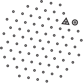
FIG. 1.: The configuration of electrons in the island for the case $N=80,A=10^{-8},U_{0}=1$, and $s=1$. A typical surface particle in a large dot has four nearest neighbors. Two particles with three and five nearest neighbors are shown by the circle and the triangle correspondingly. They represent a pair of opposite surface disclinations or a surface dislocation.

One can think about the new rows appearing in the crystalline island as of pairs of dislocations of opposite sign. In the case of the short-range interaction these defects are pushed to the surface by a huge price for elastic deformations. In the Coulomb case, described by Eq. (3), the shear modulus and, subsequently, the Young’s modulus of the crystal are relatively small. As discussed in Section V the incommensurability of the circular shape of the dot with the lattice and the inhomogeneity of the density of electrons generate in this case topological defects, disclinations and dislocations, inside the island. We argue that these defects determine the variations of the energy when the center of the confinement is fixed relative to the crystal. The number of dislocations scales as the number of crystalline rows $\sim\sqrt{N}$. This implies that a new dislocation appears every $\sim\sqrt{N}$ electrons. Due to the discreteness of these defects a single branch of the total energy corresponding to a fixed position of the center acquires a quasi-periodic correction. This periodic building up and relaxation of the elastic energy of the dot caused by the discreteness of dislocations is very similar to the variations of the electrostatic energy brought about by the discreteness of electrons, known as Coulomb blockade. Following this analogy we call the former periodic phenomenon an elastic blockade.

The elastic blockade appears to be a bit more complicated than its electrostatic counterpart. The center of the confinement can move among three distinct points of the triangular lattice mentioned above making the system switch from one energy branch to another. Such a sudden switching results in a correction to the charging energy [see Eq. (1)]:

$$\delta\Delta\approx-0.15\overline{\Delta},$$ (5)

where $\overline{\Delta}$ is the average charging energy. This reduction of the distance between the nearest Coulomb blockade peaks happens with the period $\sim\sqrt{N}$ determined by the elastic blockade. It can be thought of as an analog of merging of a few peaks observed in the case of the short-range interaction.

The optimum configurations of electrons in the parabolic confinement with the Coulomb interaction have been studied before in Ref. [6]. Our numerical results both for the energies and the configurations agree with the results of this work. However our interpretation of the results is different. The authors of Ref. [6] adopt a model in which the electrons fill in shells concentric to the perimeter of the island. We argue that in the regime studied in the numerical experiment only a narrow ring adjacent to the perimeter is concentric to it. The width of such a ring is $\sim\sqrt{R\cdot a}$. The rest of the island is filled with an almost perfect crystal. (see a Sections V and VI).

The paper is organized as follows. First we consider the case of an extremely short-range interaction [Eq. (4)], when the Young’s modulus of the crystal is very large and no lattice defects can exist in the interior of the island. This case is discussed in Sections II and III. In Section IV we report the results of the numerical solution of the problem with the Coulomb interaction [Eq. (3)]. In Section V we turn to the discussion of different kinds of defects, which can exist in a compressible island. In Section VI, we discuss the theory of the elastic blockade for the case of the Coulomb interaction. Section VII is dedicated to our conclusions.

II Short-Range interaction: Numerical Results

In this section we consider the system of $N$ electrons interacting by a strongly screened short-range potential. This limit is defined by Eq. (2) with interaction given by Eq. (4) and $a\gg s$. As it is shown later in Section III the latter condition can be realized if the interaction prefactor significantly exceeds the typical confinement energy: $U_{0}\gg AR^{2}$. At this condition the variations of the lattice constant of the crystal are negligible. This indeed can be observed in the configurations obtained in the numerical experiment. One of such a configurations is shown in Fig.1, obtained at $a\approx 13s$.

In our numerical analysis we minimized the energy functional (2) with the exponential interaction given by Eq. (4) with respect to the coordinates of electrons using a genetic algorithm similar to that outlined in Ref. [7]. Below we describe this numerical technique and the motivation for its use.

The problem at hand belongs to the vast class of problems of finding the global minimum of a multi-dimensional function, which has plenty of local minima. The well developed methods for convex differentiable functions (the conjugate gradient, Newton’s method) do not work here as they find only some local minimum. The most frequently used method in this case is the Metropolis simulated annealing technique. [6] In this method the system is modeled at some artificially introduced temperature, which is gradually decreased to a very small value. It is assumed that after this annealing the system falls into the state of the lowest energy. Although in principle in this method the system can hop from a metastable state to the ground state, in practice, if the potential barrier between them is high, the time to perform such a hop can exceed the time of the simulation.

An alternative method is the genetic algorithm, which was proved to be superior to the simulated annealing.[7] Initially five different parent configurations were obtained by relaxing random configurations using the conjugate gradient algorithm. Then these configuration were mated pairwise to obtain additional $15$ child configurations (including mating with itself), which were again relaxed using the conjugate gradient algorithm. Mating consisted in cutting two configurations into halves by a random line and then connecting those halves belonging to different parents to form a new child. From the resulting $20$ conformations (parents and children) five were chosen to be parents for the next iteration. The new parents consisted of the lowest energy configuration and the other four separated by at least the precision of the conjugate gradient. This has been done to avoid dominating the process by one conformation. During ten iterations as many as $155$ local minima were examined. The energies of the optimum conformations obtained in this way agree with those of Ref. [6] and for some $N$ are even lower. Before presenting these results we would like to discuss the method we used to process the data.

To analyze the dependence of the ground state energy $E\left(N\right)$ on the number of particles we split it into the smooth $\bar{E}\left(N\right)$ and the fluctuating component $\delta E\left(N\right)$:

$$E\left(N\right)=\bar{E}\left(N\right)+\delta E\left(N\right),$$ (6)

in the manner of Ref. [5]. The smooth component has the form $\bar{E}(N)=\eta_{1}N^{2}+\eta_{2}N+\eta_{3}N^{2/3}+\eta_{4}N^{1/2}+\eta_{5}N^{1/3}$, where the coefficients $\eta_{1}\cdots\eta_{5}$ are chosen to minimize the fluctuations. The fluctuating part is displayed in Fig. 2.

FIG. 2.: The fluctuating part of the ground state energy in the model with the exponential interaction (4) for $A=10^{-8},U_{0}=1$, and $s=1$.

The curve in Fig. 2 evidently has a quasi-periodic structure. It consists of the series of interchanging deep and shallow minima, separated by the peeks with more or less smooth slopes. We call this structure the ”Kremlin wall” for its resemblance to the embattlements on top of the walls of the Moscow Kremlin. Its period with a very good precision scales as $N^{1/2}$ and numerically is equal to the number of electrons in the outer crystalline row of the island. The amplitude of the oscillations grows with $N$ as [5]

$$\left|\delta E\right|\propto N^{\gamma},~{}~{}\gamma=0.8\pm 0.1.$$ (7)

Although the crystal in the bulk is almost perfect, its boundary is extremely irregular (see Fig. 1). It can be thought of as a superposition of various types of defects pushed against the surface by extremely large Young’s modulus, provided by the short-range interaction. These defects can be associated with the particles having an anomalous coordination number. Normally a particle on the surface of the triangular crystal has four nearest neighbors. But there are particles having a coordination number equal to three or five. These particles can be associated with positive and negative disclinations on the surface correspondingly, as their creation assumes removal (insertion) of a $\pi/3$ wedge (see Fig. 1). Dislocations on the surface are pairs of such disclinations of the opposite sign forming a dipole. At a small Young’s modulus however these defects can dive inside the island. This transition is quantitatively described in Section V.

III Short-Range interaction: a Theory

In this section we use a hard disk model to explain our numerical results obtained in the limit $U_{0}\gg AR^{2}$. To justify this model we first show that the variation of the lattice constant in the island is small in this limit:

$$\delta a=a(R)-a(0)=\frac{s}{2}\ln N\ll a(0).$$ (8)

Then we demonstrate that the interaction energy is small compared to the confinement energy and hence can be neglected.

To prove the first statement we find the pressure $\sigma_{\rm rr}$ in the crystal associated with its contraction by the external potential $Ar^{2}$. The solution can be found similar to Ref. [8]

$$\sigma_{\rm rr}=-S(\sigma)A(R^{2}-r^{2}),$$ (9)

where $S(\sigma)=(3+\sigma)/4$, $3/4\leq S(\sigma)\leq 1$, and $\sigma$ is the Poisson ratio. The solution is easy to understand for the limiting case of liquid $\sigma\rightarrow 1$, when $\sigma_{ik}=-p\delta_{ik}$, $p$ being pressure. In this case $p$ is of purely hydrostatic origin:

$$\frac{dp(r)}{dr}=-2Arn(r).$$ (10)

Assuming the density $n(r)$ to be uniform and $p(R)=0$ we obtain the following solution:

$$p(r)=An(R^{2}-r^{2}),$$ (11)

which agrees with Eq. (9) taken at $\sigma=1$. The forces produced by this pressure have to be balanced by the interaction forces between particles:

$$f\sim\sigma_{\rm rr}a\sim An(R^{2}-r^{2})a\sim\frac{U_{0}}{s}e^{-a/s}.$$ (12)

In this equation we assumed $S(\sigma)\sim 1$. From this condition we obtain the following result for the lattice spacing in the island:

$$a(r)\approx s\ln\left[\frac{U_{0}}{A\left(R^{2}-r^{2}\right)}\right].$$ (13)

The difference between the lattice spacing on the boundary and in the center can be readily obtained:

$$\delta a\approx s\ln\left(\frac{U_{0}}{ARa}\right)-s\ln\left(\frac{U_{0}}{AR^{2}}\right)=s\ln\frac{R}{a}=\frac{s}{2}\ln N.$$ (14)

Comparing (13) and (14) one can see that the case $a\gg\delta a$ can be realized when $U_{0}\gg AR^{2}$. This implies that the prefactor of the interaction potential has to be large. In this case the nearest particles are far away from each other where the exponential interaction is very steep. This eliminates significant changes in the interparticle distance.

Although the derivative of the interaction potential is important in determining the lattice spacing the typical value of interaction energy in this case is very small. The characteristic interaction energy per particle can be estimated as: $E_{\rm nn}\sim U_{0}\exp(-a/s)$. From Eq. (12) we conclude that

$$U_{0}e^{-a/s}\lesssim\frac{s}{a}AR^{2}.$$ (15)

Hence in the considered regime $a\gg s$ the interaction energy indeed can be neglected.

It is plausible then to accept the hard disk model to explain our numerical results obtained for this case. We assume therefore that the interaction has the form:

$$U(r)=\left\{\begin{array}[]{ll}{\displaystyle\infty,}&{r<a,}\\ \\ {\displaystyle 0,}&{r\geq a.}\end{array}\right.$$ (16)

In this model the interaction energy is zero and the total energy of the system can be written as:

$$E=A\sum_{i=1}^{N}{\mathchoice{{\hbox{\boldmath$\displaystyle r$}}}{{\hbox{\boldmath$\textstyle r$}}}{{\hbox{\boldmath$\scriptstyle r$}}}{{\hbox{\boldmath$\scriptscriptstyle r$}}}}_{i}^{2},$$ (17)

where ${\mathchoice{{\hbox{\boldmath$\displaystyle r$}}}{{\hbox{\boldmath$\textstyle r$}}}{{\hbox{\boldmath$\scriptstyle r$}}}{{\hbox{\boldmath$\scriptscriptstyle r$}}}}_{i}$ belong to the triangular lattice, with the lattice spacing equal to the radius of the interaction $a$. This energy formally coincides with the moment of inertia of the system of $N$ particles of mass $A$. Hence to find the minimum energy configuration one has to cut a piece from the triangular crystal that has a minimum moment of inertia. This piece must contain the given number of particles $N$. The average values of the total energy, chemical potential and the charging energy are given by:

$$\begin{array}[]{l}{\bar{E}=AN\cdot R^{2}/2=AN^{2}/2\pi n}\\ \\ {\bar{\mu}=d\bar{E}/dN=AN/\pi n}\\ \\ {\bar{\Delta}=d\bar{\mu}/dN=A/\pi n},\end{array}$$ (18)

where $R$ is the average radius of the circle, $n\pi R^{2}=N$, $n=2/a^{2}\sqrt{3}$ is the concentration of lattice sites.

A similar problem has been considered in the literature in the context of the so-called circle problem. The problem is to find the fluctuations of the number of particles belonging to some lattice inside of a circle of radius $R$ (see Ref. [9]). The quantity which has been studied is the deviation of the number of particles from its average value:

$$\delta N(R)\equiv N(R)-n\pi R^{2},$$ (19)

where $n\pi R^{2}=\bar{N}$ is the average number of particles in the circle. The classical circle problem which goes back to Gauss is to find the uniform bound for $|\delta N(R)|$. The best result in this direction is[9]

$$|\delta N|\leq C_{\epsilon}R^{46/73+\epsilon}\sim\bar{N}^{23/73+\epsilon/2}$$ (20)

Here $C_{\epsilon}$ is a $R$-independent constant and $\epsilon>0$. A simple estimate for these fluctuations can be obtained from the assumption that they occur around the perimeter of the circle [9] in the strip of width of the order of the lattice spacing $a$. The number of such points $N_{\rm per}\sim R/a$ and the fluctuations are

$$\delta N\sim\sqrt{N_{\rm per}}\sim\sqrt{R/a}\sim\bar{N}^{1/4}.$$ (21)

This estimate may imply a pseudo-random behavior of $\delta N$. Notice that it agrees with the uniform upper bound (20) as $23/73>1/4$.

Ref. [9] also considers the distribution of $\delta N$. It was found that the distribution function is non-Gaussian:

$$p(\delta N)\lesssim\exp\left(-\delta N^{4}/\bar{N}\right),$$ (22)

with the mean square deviation given by Eq. (21). It was also noted that $\delta N(R)$ in addition to be pseudo-random is almost periodic function of the radius.

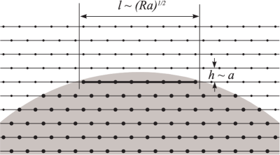
FIG. 3.: The circular island (gray) covering the crystalline rows, shown by lines. The lattice points within the circle are shown by larger disks than those outside. Every time the circle intersects a new row a new terrace appears. One of such terraces is shown by the bold segment.

Below we will concentrate on the periodicity of $\delta N(R)$, rather than on its randomness. In essence we would like to find the average of $\delta N(R)$ over many periods and understand the nature of its oscillations. Then the question about the deviations from this average becomes relevant. Our analysis shows that the oscillations are associated with the periodic intersections of the circle with the crystalline rows (see Fig. 3). At the moment of intersection an anomalously large number of particles can be put into the circle. This brings about an increase in the function $\delta N(R)$ every time the circle hits a new crystalline row. This increase is accompanied by a decrease later in the period as the average value of $\delta N$ is zero. To illustrate this point consider the triangular lattice (Fig. 3). In this case for the most part the oscillations of $\delta N$ are associated with the collisions of the circle with the main crystalline rows, ($\sqrt{3},1$) plus other five obtained by $\pi/3$ rotations, separated by $h=a\sqrt{3}/2$. Hence the variations of $\delta N$ associated with these rows have a period in $R$ equal to $T_{R}=h$. One can collapse $\delta N$ from many such periods into one and average over all of them. To do this we first define a normalized variation of the number of particles:

$$\delta\eta(R)\equiv\frac{\delta N}{\sqrt{R}}$$ (23)

According to Eq. (21) the average amplitude of this function does not change with $R$. To extract the component of this function having the period $T_{R}=h$ we average it over many such periods:

$$\overline{\delta\eta}\left(R\right)=\lim_{M\rightarrow\infty}\left[\frac{1}{M}\sum_{m=0}^{M}\delta\eta\left(T_{R}m+R\right)\right].$$ (24)

Thus obtained function $\overline{\delta N}(R)\equiv\overline{\delta\eta}\left(R\right)\sqrt{R}$ is shown in Fig. 4 by a smooth line. The actual $\delta N(R)$ is also presented in this figure to show that its main variation is indeed associated with the aforementioned period.

FIG. 4.: The averaged oscillations of the number of particles as a function of the radius of the circle (bold smooth line) and the actual value, observed in the numerical simulation on the lattice (thin rough line). The center of the circle is located at one of the lattice sites.

Before embarking into the calculation of the $\overline{\delta N}$ we would like to mention that other crystalline planes produce similar oscillations. These oscillations have a period that is smaller than $h$ and can be incommensurate to it. The amplitude of these satellite oscillations is numerically smaller than the main one and hence they will be neglected in this paper. All the periodicities added together produce a complex fractal curve shown in Fig. 4.

Before getting into details of the averaging we would like to show a simple way to estimate the amplitude of these oscillations. Look at Fig. 3. The collision of a crystalline row with the circle results in the formation of the “terrace” on the surface of the crystal bounded by the circle. The average length of such a “terrace” is

$$l\sim\sqrt{R\cdot a}.$$ (25)

The number of crystalline sites in such a “terrace” provides an estimate for the variations in the number of particles inside the circle:

$$\delta N=l/a\sim\sqrt{R/a}.$$ (26)

This estimate agrees with Eq. (21). However, it is based on the existence of the ordered periodic structure in $\delta N$.

This argument allows us to estimate the amplitude of the oscillations of the total energy (17). Indeed, we have found the oscillations of the number of particles as a function of radius or, in other words, of the chemical potential $\mu=AR^{2}$. Now it easy to calculate the related oscillation of the chemical potential as a function of the number of particles. To this end we notice that if the oscillations are weak they are simply proportional to each other:

$$\delta\mu=-\delta N/\bar{\nu},$$ (27)

where $\bar{\nu}=1/\bar{\Delta}$ is the average density of states. The period of $\delta\mu(N)$ is related to the period of $\delta N(R)$ in the obvious way: $T_{N}=dN/dR\cdot T_{R}=\pi nRh\sim\sqrt{N}$. Now the oscillating part of the total energy can be easily estimated:

$$\begin{array}[]{ll}{\delta E(N)}&{=\int dN\delta\mu(N)}\\ \\ {}&{\sim T_{N}\cdot\delta N\bar{\Delta}\sim Aa^{2}N^{3/4}}.\end{array}$$ (28)

Notice that both the periodicity and amplitude of the oscillations given by this estimate agree with our numerical results (7). Below we will calculate the form of these oscillations averaged over many periods.

We now turn to the calculation of $\overline{\delta N}(R)$. We follow the guidelines of Ref. [9]. Assume that the center of the circle is located at point $\mathchoice{{\hbox{\boldmath$\displaystyle r$}}}{{\hbox{\boldmath$\textstyle r$}}}{{\hbox{\boldmath$\scriptstyle r$}}}{{\hbox{\boldmath$\scriptscriptstyle r$}}}_{0}$ reduced to Bravais unit cell. The number of particles in the circle can be expressed through the sum over the lattice points ${\mathchoice{{\hbox{\boldmath$\displaystyle R$}}}{{\hbox{\boldmath$\textstyle R$}}}{{\hbox{\boldmath$\scriptstyle R$}}}{{\hbox{\boldmath$\scriptscriptstyle R$}}}}_{l}$:

$$\begin{array}[]{ll}{\delta N(R)}&{=N-n\pi R^{2}}\\ \\ {}&{\displaystyle=\sum_{{\mathchoice{{\hbox{\boldmath$\displaystyle R$}}}{{\hbox{\boldmath$\textstyle R$}}}{{\hbox{\boldmath$\scriptstyle R$}}}{{\hbox{\boldmath$\scriptscriptstyle R$}}}}_{l}}f\left({\mathchoice{{\hbox{\boldmath$\displaystyle R$}}}{{\hbox{\boldmath$\textstyle R$}}}{{\hbox{\boldmath$\scriptstyle R$}}}{{\hbox{\boldmath$\scriptscriptstyle R$}}}}_{l}\right)-\int nd^{2}rf\left({\mathchoice{{\hbox{\boldmath$\displaystyle r$}}}{{\hbox{\boldmath$\textstyle r$}}}{{\hbox{\boldmath$\scriptstyle r$}}}{{\hbox{\boldmath$\scriptscriptstyle r$}}}}\right),}\end{array}$$ (29)

where

$$f({\mathchoice{{\hbox{\boldmath$\displaystyle r$}}}{{\hbox{\boldmath$\textstyle r$}}}{{\hbox{\boldmath$\scriptstyle r$}}}{{\hbox{\boldmath$\scriptscriptstyle r$}}}})=\left\{\begin{array}[]{ll}{\displaystyle 1,}&{\left|{\mathchoice{{\hbox{\boldmath$\displaystyle r$}}}{{\hbox{\boldmath$\textstyle r$}}}{{\hbox{\boldmath$\scriptstyle r$}}}{{\hbox{\boldmath$\scriptscriptstyle r$}}}}-{\mathchoice{{\hbox{\boldmath$\displaystyle r$}}}{{\hbox{\boldmath$\textstyle r$}}}{{\hbox{\boldmath$\scriptstyle r$}}}{{\hbox{\boldmath$\scriptscriptstyle r$}}}}_{0}\right|\leq R,}\\ \\ {\displaystyle 0,}&{\left|{\mathchoice{{\hbox{\boldmath$\displaystyle r$}}}{{\hbox{\boldmath$\textstyle r$}}}{{\hbox{\boldmath$\scriptstyle r$}}}{{\hbox{\boldmath$\scriptscriptstyle r$}}}}-{\mathchoice{{\hbox{\boldmath$\displaystyle r$}}}{{\hbox{\boldmath$\textstyle r$}}}{{\hbox{\boldmath$\scriptstyle r$}}}{{\hbox{\boldmath$\scriptscriptstyle r$}}}}_{0}\right|>R.}\end{array}\right.$$ (30)

Using the Poisson summation formula, Eq. (29) can be rewritten as follows:

$$\delta N(R)=n\sum_{{\mathchoice{{\hbox{\boldmath$\displaystyle Q$}}}{{\hbox{\boldmath$\textstyle Q$}}}{{\hbox{\boldmath$\scriptstyle Q$}}}{{\hbox{\boldmath$\scriptscriptstyle Q$}}}}_{i}\neq 0}\tilde{f}\left({\mathchoice{{\hbox{\boldmath$\displaystyle Q$}}}{{\hbox{\boldmath$\textstyle Q$}}}{{\hbox{\boldmath$\scriptstyle Q$}}}{{\hbox{\boldmath$\scriptscriptstyle Q$}}}}_{i}\right),$$ (31)

where the summation is assumed over the reciprocal lattice vectors ${\mathchoice{{\hbox{\boldmath$\displaystyle Q$}}}{{\hbox{\boldmath$\textstyle Q$}}}{{\hbox{\boldmath$\scriptstyle Q$}}}{{\hbox{\boldmath$\scriptscriptstyle Q$}}}}_{i}$ and $\tilde{f}\left({\mathchoice{{\hbox{\boldmath$\displaystyle q$}}}{{\hbox{\boldmath$\textstyle q$}}}{{\hbox{\boldmath$\scriptstyle q$}}}{{\hbox{\boldmath$\scriptscriptstyle q$}}}}\right)=2\pi RJ_{1}(\left|{\mathchoice{{\hbox{\boldmath$\displaystyle q$}}}{{\hbox{\boldmath$\textstyle q$}}}{{\hbox{\boldmath$\scriptstyle q$}}}{{\hbox{\boldmath$\scriptscriptstyle q$}}}}\right|R)/\left|{\mathchoice{{\hbox{\boldmath$\displaystyle q$}}}{{\hbox{\boldmath$\textstyle q$}}}{{\hbox{\boldmath$\scriptstyle q$}}}{{\hbox{\boldmath$\scriptscriptstyle q$}}}}\right|\cdot\exp(-i\mathchoice{{\hbox{\boldmath$\displaystyle qr$}}}{{\hbox{\boldmath$\textstyle qr$}}}{{\hbox{\boldmath$\scriptstyle qr$}}}{{\hbox{\boldmath$\scriptscriptstyle qr$}}}_{0})$ is the Fourier transform of function (30), with $J_{1}(x)$ being the Bessel function. For the normalized variation of number of particles  (23) we then obtain:

$$\delta\eta(R)=2\pi n\sqrt{R}\sum_{{\mathchoice{{\hbox{\boldmath$\displaystyle Q$}}}{{\hbox{\boldmath$\textstyle Q$}}}{{\hbox{\boldmath$\scriptstyle Q$}}}{{\hbox{\boldmath$\scriptscriptstyle Q$}}}}_{i}\neq 0}\frac{J_{1}(\left|{\mathchoice{{\hbox{\boldmath$\displaystyle Q$}}}{{\hbox{\boldmath$\textstyle Q$}}}{{\hbox{\boldmath$\scriptstyle Q$}}}{{\hbox{\boldmath$\scriptscriptstyle Q$}}}}_{i}\right|R)}{\left|{\mathchoice{{\hbox{\boldmath$\displaystyle Q$}}}{{\hbox{\boldmath$\textstyle Q$}}}{{\hbox{\boldmath$\scriptstyle Q$}}}{{\hbox{\boldmath$\scriptscriptstyle Q$}}}}_{i}\right|}e^{-i\mathchoice{{\hbox{\boldmath$\displaystyle Q$}}}{{\hbox{\boldmath$\textstyle Q$}}}{{\hbox{\boldmath$\scriptstyle Q$}}}{{\hbox{\boldmath$\scriptscriptstyle Q$}}}_{i}\mathchoice{{\hbox{\boldmath$\displaystyle r$}}}{{\hbox{\boldmath$\textstyle r$}}}{{\hbox{\boldmath$\scriptstyle r$}}}{{\hbox{\boldmath$\scriptscriptstyle r$}}}_{0}}.$$ (32)

The limit in Eq. (24) can be most easily evaluated upon noticing that $J_{1}(x)\approx\sqrt{2/\pi x}\cos\left(x-3\pi/4\right)$, when $x\gg 1$. Changing the order of summation over $\mathchoice{{\hbox{\boldmath$\displaystyle Q$}}}{{\hbox{\boldmath$\textstyle Q$}}}{{\hbox{\boldmath$\scriptstyle Q$}}}{{\hbox{\boldmath$\scriptscriptstyle Q$}}}_{i}$ and $m$ we obtain:

$$\begin{array}[]{l}{\displaystyle\overline{\delta\eta}\left(R\right)=\lim_{M\rightarrow\infty}\left[\frac{1}{M}2\pi n\sum_{{\mathchoice{{\hbox{\boldmath$\displaystyle Q$}}}{{\hbox{\boldmath$\textstyle Q$}}}{{\hbox{\boldmath$\scriptstyle Q$}}}{{\hbox{\boldmath$\scriptscriptstyle Q$}}}}_{i}\neq 0}\sum_{m=0}^{M}\sqrt{\frac{2}{\pi}}\right.}\\ \\ {\displaystyle\left.\times\frac{\cos\left(\left|{\mathchoice{{\hbox{\boldmath$\displaystyle Q$}}}{{\hbox{\boldmath$\textstyle Q$}}}{{\hbox{\boldmath$\scriptstyle Q$}}}{{\hbox{\boldmath$\scriptscriptstyle Q$}}}}_{i}\right|T_{R}m+\left|{\mathchoice{{\hbox{\boldmath$\displaystyle Q$}}}{{\hbox{\boldmath$\textstyle Q$}}}{{\hbox{\boldmath$\scriptstyle Q$}}}{{\hbox{\boldmath$\scriptscriptstyle Q$}}}}_{i}\right|R-3\pi/4\right)}{\left|{\mathchoice{{\hbox{\boldmath$\displaystyle Q$}}}{{\hbox{\boldmath$\textstyle Q$}}}{{\hbox{\boldmath$\scriptstyle Q$}}}{{\hbox{\boldmath$\scriptscriptstyle Q$}}}}_{i}\right|^{3/2}}e^{-i\mathchoice{{\hbox{\boldmath$\displaystyle Q$}}}{{\hbox{\boldmath$\textstyle Q$}}}{{\hbox{\boldmath$\scriptstyle Q$}}}{{\hbox{\boldmath$\scriptscriptstyle Q$}}}_{i}\mathchoice{{\hbox{\boldmath$\displaystyle r$}}}{{\hbox{\boldmath$\textstyle r$}}}{{\hbox{\boldmath$\scriptstyle r$}}}{{\hbox{\boldmath$\scriptscriptstyle r$}}}_{0}}\right]}\end{array}$$ (33)

To evaluate the sum over $m$ we again can use the Poisson summation formula, which establishes a selection rule for the values of the wave-vector $\mathchoice{{\hbox{\boldmath$\displaystyle Q$}}}{{\hbox{\boldmath$\textstyle Q$}}}{{\hbox{\boldmath$\scriptstyle Q$}}}{{\hbox{\boldmath$\scriptscriptstyle Q$}}}_{i}$:

$$\left|{\mathchoice{{\hbox{\boldmath$\displaystyle Q$}}}{{\hbox{\boldmath$\textstyle Q$}}}{{\hbox{\boldmath$\scriptstyle Q$}}}{{\hbox{\boldmath$\scriptscriptstyle Q$}}}}_{i}\right|T_{R}=2\pi n,$$ (34)

where $n$ is an integer. The reciprocal lattice vectors are representable in the form $\mathchoice{{\hbox{\boldmath$\displaystyle Q$}}}{{\hbox{\boldmath$\textstyle Q$}}}{{\hbox{\boldmath$\scriptstyle Q$}}}{{\hbox{\boldmath$\scriptscriptstyle Q$}}}_{i}=Q_{0}\left(k_{1}\sqrt{3}/2,k_{1}/2+k_{2}\right)$, where $Q_{0}=4\pi/a\sqrt{3}$ and $k_{1,2}$ are integers. Equation (34) can be rewritten in term of $k_{1,2}$ in the following way: $3k_{1}^{2}+(k_{1}+2k_{2})^{2}=4n^{2}$, which is a Diophantine equation. It has a trivial set of solutions, $k_{1}=0$, $k_{2}=n$ plus five others obtained from it by $\pi/3$ rotations. They correspond to the collisions of the circle with the main sequence of the crystalline rows, separated by $T_{R}$. These solutions will be taken into account below. The other solutions of Eq. (34) are more sparse in the $Q$-space, and hence produce smaller than $T_{R}$ periods in the real space. They correspond to the collisions with other crystalline lines. They produce numerically smaller variations than the main sequence and will be disregarded below. Thus we conclude that

$$\begin{array}[]{l}{\displaystyle\lim_{M\rightarrow\infty}\left[\frac{1}{M}\sum_{m=0}^{M}\cos\left(\left|{\mathchoice{{\hbox{\boldmath$\displaystyle Q$}}}{{\hbox{\boldmath$\textstyle Q$}}}{{\hbox{\boldmath$\scriptstyle Q$}}}{{\hbox{\boldmath$\scriptscriptstyle Q$}}}}_{i}\right|T_{R}m+\left|{\mathchoice{{\hbox{\boldmath$\displaystyle Q$}}}{{\hbox{\boldmath$\textstyle Q$}}}{{\hbox{\boldmath$\scriptstyle Q$}}}{{\hbox{\boldmath$\scriptscriptstyle Q$}}}}_{i}\right|R-3\pi/4\right)\right]}\\ \\ {\displaystyle=\sum_{\mathchoice{{\hbox{\boldmath$\displaystyle\tilde{Q}$}}}{{\hbox{\boldmath$\textstyle\tilde{Q}$}}}{{\hbox{\boldmath$\scriptstyle\tilde{Q}$}}}{{\hbox{\boldmath$\scriptscriptstyle\tilde{Q}$}}}_{i}}\delta_{\mathchoice{{\hbox{\boldmath$\displaystyle\tilde{Q}$}}}{{\hbox{\boldmath$\textstyle\tilde{Q}$}}}{{\hbox{\boldmath$\scriptstyle\tilde{Q}$}}}{{\hbox{\boldmath$\scriptscriptstyle\tilde{Q}$}}}_{i},\mathchoice{{\hbox{\boldmath$\displaystyle Q$}}}{{\hbox{\boldmath$\textstyle Q$}}}{{\hbox{\boldmath$\scriptstyle Q$}}}{{\hbox{\boldmath$\scriptscriptstyle Q$}}}_{i}}\cos\left(\left|{\mathchoice{{\hbox{\boldmath$\displaystyle Q$}}}{{\hbox{\boldmath$\textstyle Q$}}}{{\hbox{\boldmath$\scriptstyle Q$}}}{{\hbox{\boldmath$\scriptscriptstyle Q$}}}}_{i}\right|R-3\pi/4\right),}\end{array}$$ (35)

where $\mathchoice{{\hbox{\boldmath$\displaystyle\tilde{Q}$}}}{{\hbox{\boldmath$\textstyle\tilde{Q}$}}}{{\hbox{\boldmath$\scriptstyle\tilde{Q}$}}}{{\hbox{\boldmath$\scriptscriptstyle\tilde{Q}$}}}_{i}$ are solutions of (34) with the reservations mentioned above. The remaining summation over $\mathchoice{{\hbox{\boldmath$\displaystyle Q$}}}{{\hbox{\boldmath$\textstyle Q$}}}{{\hbox{\boldmath$\scriptstyle Q$}}}{{\hbox{\boldmath$\scriptscriptstyle Q$}}}_{i}$ is easily performed and we obtain finally the result for the average variation of the number of particles:

$$\overline{\delta N_{\mathchoice{{\hbox{\boldmath$\displaystyle r$}}}{{\hbox{\boldmath$\textstyle r$}}}{{\hbox{\boldmath$\scriptstyle r$}}}{{\hbox{\boldmath$\scriptscriptstyle r$}}}_{0}}}\left(R\right)=\sum_{i=1}^{6}\overline{\delta N_{0}}\left(R-\mathchoice{{\hbox{\boldmath$\displaystyle\hat{e}$}}}{{\hbox{\boldmath$\textstyle\hat{e}$}}}{{\hbox{\boldmath$\scriptstyle\hat{e}$}}}{{\hbox{\boldmath$\scriptscriptstyle\hat{e}$}}}_{i}\mathchoice{{\hbox{\boldmath$\displaystyle r$}}}{{\hbox{\boldmath$\textstyle r$}}}{{\hbox{\boldmath$\scriptstyle r$}}}{{\hbox{\boldmath$\scriptscriptstyle r$}}}_{0}\right),$$ (36)

where $\mathchoice{{\hbox{\boldmath$\displaystyle\hat{e}$}}}{{\hbox{\boldmath$\textstyle\hat{e}$}}}{{\hbox{\boldmath$\scriptstyle\hat{e}$}}}{{\hbox{\boldmath$\scriptscriptstyle\hat{e}$}}}_{i}$ are the unitary vectors normal to the six main crystalline rows, $\mathchoice{{\hbox{\boldmath$\displaystyle\hat{e}$}}}{{\hbox{\boldmath$\textstyle\hat{e}$}}}{{\hbox{\boldmath$\scriptstyle\hat{e}$}}}{{\hbox{\boldmath$\scriptscriptstyle\hat{e}$}}}_{i}=\hat{U}^{i}(\sqrt{3}/2,1/2)$, $\hat{U}$ is the $\pi/3$ rotation, $i=0,\ldots,5$. Function $\overline{\delta N_{0}}$ determines the oscillations produced by one set of rows if the center of the circle $\mathchoice{{\hbox{\boldmath$\displaystyle r$}}}{{\hbox{\boldmath$\textstyle r$}}}{{\hbox{\boldmath$\scriptstyle r$}}}{{\hbox{\boldmath$\scriptscriptstyle r$}}}_{0}$ coincides with one of the lattice sites:

$$\overline{\delta N_{0}}\left(R\right)=\frac{2^{3/4}3^{3/8}}{\pi^{1/4}}\left[\bar{N}(R)\right]^{1/4}\zeta\left(-\frac{1}{2},\frac{R}{T_{R}}\right).$$ (37)

Here

$$\zeta\left(z,q\right)=\frac{2\Gamma(1-z)}{\left(2\pi\right)^{1-z}}\sum_{k=1}^{\infty}\frac{\sin\left(2\pi kq+z\pi/2\right)}{k^{1-z}},$$ (38)

is the generalized Riemann zeta-function. [10] In addition to the numerical coefficient in Eq. (37) we obtained the overall amplitude $N^{1/4}$, which agrees with our qualitative analysis, and the oscillating part $\zeta\left(-1/2,R/T_{R}\right)$, which has an amplitude of the order of unity. In Fig. 4 $\overline{\delta N}_{\mathchoice{{\hbox{\boldmath$\displaystyle r$}}}{{\hbox{\boldmath$\textstyle r$}}}{{\hbox{\boldmath$\scriptstyle r$}}}{{\hbox{\boldmath$\scriptscriptstyle r$}}}_{0}=0}$ is shown by a smooth line. It is clear from Eq. (36) that six sequences of the crystalline rows contribute to oscillations independently, with $\mathchoice{{\hbox{\boldmath$\displaystyle\hat{e}$}}}{{\hbox{\boldmath$\textstyle\hat{e}$}}}{{\hbox{\boldmath$\scriptstyle\hat{e}$}}}{{\hbox{\boldmath$\scriptscriptstyle\hat{e}$}}}_{i}\mathchoice{{\hbox{\boldmath$\displaystyle r$}}}{{\hbox{\boldmath$\textstyle r$}}}{{\hbox{\boldmath$\scriptstyle r$}}}{{\hbox{\boldmath$\scriptscriptstyle r$}}}_{0}$ determining a “delay” produced by the displacement of the center of the circle from a lattice site.

We would like now to calculate the oscillations of the total energy of the incompressible island. First, as parameters of the problem we will use $\mathchoice{{\hbox{\boldmath$\displaystyle r$}}}{{\hbox{\boldmath$\textstyle r$}}}{{\hbox{\boldmath$\scriptstyle r$}}}{{\hbox{\boldmath$\scriptscriptstyle r$}}}_{0}$ and $R$. This implies that we will have a given value of the chemical potential in the island $\mu=AR^{2}$. The relevant thermodynamic potential in this case is $\Omega_{\mathchoice{{\hbox{\boldmath$\displaystyle r$}}}{{\hbox{\boldmath$\textstyle r$}}}{{\hbox{\boldmath$\scriptstyle r$}}}{{\hbox{\boldmath$\scriptscriptstyle r$}}}_{0}}(\mu)$. We will evaluate this potential and optimize it with respect to $r_{0}$. We will then use the theorem of small increments to find $E(N)$. This function will indeed be similar to the Kremlin wall structure displayed in Fig. 2.

The first step in this program is realized similar to obtaining $\overline{\delta N}$. We apply the method used above to the function

$$\Omega(R)=E(R)-\mu N,~{}~{}\mu=AR^{2}.$$ (39)

The average value of this function is negative:

$$\bar{\Omega}=-AN\cdot R^{2}/2=-\bar{E},$$ (40)

(compare to Eq. (18)). The deviation of the potential from the average is given by

$$\begin{array}[]{ll}{\delta\Omega(R)}&{=\delta E(R)-AR^{2}\delta N(R)}\\ \\ {}&{\displaystyle=\sum_{{\mathchoice{{\hbox{\boldmath$\displaystyle R$}}}{{\hbox{\boldmath$\textstyle R$}}}{{\hbox{\boldmath$\scriptstyle R$}}}{{\hbox{\boldmath$\scriptscriptstyle R$}}}}_{l}}g\left({\mathchoice{{\hbox{\boldmath$\displaystyle R$}}}{{\hbox{\boldmath$\textstyle R$}}}{{\hbox{\boldmath$\scriptstyle R$}}}{{\hbox{\boldmath$\scriptscriptstyle R$}}}}_{l}\right)-\int nd^{2}rg\left({\mathchoice{{\hbox{\boldmath$\displaystyle r$}}}{{\hbox{\boldmath$\textstyle r$}}}{{\hbox{\boldmath$\scriptstyle r$}}}{{\hbox{\boldmath$\scriptscriptstyle r$}}}}\right)-AR^{2}\delta N(R),}\end{array}$$ (41)

where

$$g({\mathchoice{{\hbox{\boldmath$\displaystyle r$}}}{{\hbox{\boldmath$\textstyle r$}}}{{\hbox{\boldmath$\scriptstyle r$}}}{{\hbox{\boldmath$\scriptscriptstyle r$}}}})=\left\{\begin{array}[]{ll}{\displaystyle A({\mathchoice{{\hbox{\boldmath$\displaystyle r$}}}{{\hbox{\boldmath$\textstyle r$}}}{{\hbox{\boldmath$\scriptstyle r$}}}{{\hbox{\boldmath$\scriptscriptstyle r$}}}}-{\mathchoice{{\hbox{\boldmath$\displaystyle r$}}}{{\hbox{\boldmath$\textstyle r$}}}{{\hbox{\boldmath$\scriptstyle r$}}}{{\hbox{\boldmath$\scriptscriptstyle r$}}}}_{0})^{2},}&{\left|{\mathchoice{{\hbox{\boldmath$\displaystyle r$}}}{{\hbox{\boldmath$\textstyle r$}}}{{\hbox{\boldmath$\scriptstyle r$}}}{{\hbox{\boldmath$\scriptscriptstyle r$}}}}-{\mathchoice{{\hbox{\boldmath$\displaystyle r$}}}{{\hbox{\boldmath$\textstyle r$}}}{{\hbox{\boldmath$\scriptstyle r$}}}{{\hbox{\boldmath$\scriptscriptstyle r$}}}}_{0}\right|\leq R,}\\ \\ {\displaystyle 0,}&{\left|{\mathchoice{{\hbox{\boldmath$\displaystyle r$}}}{{\hbox{\boldmath$\textstyle r$}}}{{\hbox{\boldmath$\scriptstyle r$}}}{{\hbox{\boldmath$\scriptscriptstyle r$}}}}-{\mathchoice{{\hbox{\boldmath$\displaystyle r$}}}{{\hbox{\boldmath$\textstyle r$}}}{{\hbox{\boldmath$\scriptstyle r$}}}{{\hbox{\boldmath$\scriptscriptstyle r$}}}}_{0}\right|>R.}\end{array}\right.$$ (42)

Using

$$\tilde{g}\left({\mathchoice{{\hbox{\boldmath$\displaystyle q$}}}{{\hbox{\boldmath$\textstyle q$}}}{{\hbox{\boldmath$\scriptstyle q$}}}{{\hbox{\boldmath$\scriptscriptstyle q$}}}}\right)=\left[\frac{2\pi AR^{3}}{q}J_{1}(\left|{\mathchoice{{\hbox{\boldmath$\displaystyle q$}}}{{\hbox{\boldmath$\textstyle q$}}}{{\hbox{\boldmath$\scriptstyle q$}}}{{\hbox{\boldmath$\scriptscriptstyle q$}}}}\right|R)-\frac{4\pi AR^{2}}{q^{2}}J_{2}(\left|{\mathchoice{{\hbox{\boldmath$\displaystyle q$}}}{{\hbox{\boldmath$\textstyle q$}}}{{\hbox{\boldmath$\scriptstyle q$}}}{{\hbox{\boldmath$\scriptscriptstyle q$}}}}\right|R)\right]e^{-i\mathchoice{{\hbox{\boldmath$\displaystyle qr$}}}{{\hbox{\boldmath$\textstyle qr$}}}{{\hbox{\boldmath$\scriptstyle qr$}}}{{\hbox{\boldmath$\scriptscriptstyle qr$}}}_{0}},$$ (43)

one can obtain the oscillations of the thermodynamic potential in exactly the same manner as those of the number of particles. To this end, as it follows from (28), one has to average the normalized variations of potential: $\delta\omega\equiv\delta\Omega/R^{3/2}$ (compare to (23)). Eventually we obtain

$$\overline{\delta\Omega_{\mathchoice{{\hbox{\boldmath$\displaystyle r$}}}{{\hbox{\boldmath$\textstyle r$}}}{{\hbox{\boldmath$\scriptstyle r$}}}{{\hbox{\boldmath$\scriptscriptstyle r$}}}_{0}}}\left(R\right)=\sum_{i=1}^{6}\overline{\delta\Omega_{0}}\left(R-\mathchoice{{\hbox{\boldmath$\displaystyle\hat{e}$}}}{{\hbox{\boldmath$\textstyle\hat{e}$}}}{{\hbox{\boldmath$\scriptstyle\hat{e}$}}}{{\hbox{\boldmath$\scriptscriptstyle\hat{e}$}}}_{i}\mathchoice{{\hbox{\boldmath$\displaystyle r$}}}{{\hbox{\boldmath$\textstyle r$}}}{{\hbox{\boldmath$\scriptstyle r$}}}{{\hbox{\boldmath$\scriptscriptstyle r$}}}_{0}\right),$$ (44)

where

$$\overline{\delta\Omega_{0}}\left(R\right)=-\bar{\Delta}\frac{\pi^{1/4}2^{9/4}}{3^{3/8}}\left[\bar{N}(R)\right]^{3/4}\zeta\left(-\frac{3}{2},\frac{R}{T_{R}}\right),$$ (45)

is the function describing the oscillations if the center of the circle coincides with one of the lattice sites. Its amplitude agrees with our presumption (28). Notice that $\overline{\delta\Omega_{\mathchoice{{\hbox{\boldmath$\displaystyle r$}}}{{\hbox{\boldmath$\textstyle r$}}}{{\hbox{\boldmath$\scriptstyle r$}}}{{\hbox{\boldmath$\scriptscriptstyle r$}}}_{0}}}$ given by (44) is in fact a function of the chemical potential as the latter is related to the radius by $\mu=AR^{2}$. This function for $\mathchoice{{\hbox{\boldmath$\displaystyle r$}}}{{\hbox{\boldmath$\textstyle r$}}}{{\hbox{\boldmath$\scriptstyle r$}}}{{\hbox{\boldmath$\scriptscriptstyle r$}}}_{0}=0$ is shown in Fig. 5.

FIG. 5.: The averaged oscillations of the thermodynamic potential $\Omega$ as a function of the radius of the circle (bold smooth line) and the values actually observed in the numerical simulation (thin rough line). The center of the circle is located at one of the lattice sites.

The next step is to minimize it with respect to $\mathchoice{{\hbox{\boldmath$\displaystyle r$}}}{{\hbox{\boldmath$\textstyle r$}}}{{\hbox{\boldmath$\scriptstyle r$}}}{{\hbox{\boldmath$\scriptscriptstyle r$}}}_{0}$. To do this we notice that $\overline{\delta\Omega_{\mathchoice{{\hbox{\boldmath$\displaystyle r$}}}{{\hbox{\boldmath$\textstyle r$}}}{{\hbox{\boldmath$\scriptstyle r$}}}{{\hbox{\boldmath$\scriptscriptstyle r$}}}_{0}}}$ as a function of $\mathchoice{{\hbox{\boldmath$\displaystyle r$}}}{{\hbox{\boldmath$\textstyle r$}}}{{\hbox{\boldmath$\scriptstyle r$}}}{{\hbox{\boldmath$\scriptscriptstyle r$}}}_{0}$ must have the same symmetry as the lattice. Hence its extrema have to be located at points denoted in Fig. 6a by A, B, and C, unaffected by the transformations of the symmetry. Those are the points coinciding with a lattice site, the center of the triangular face, and the point half-way between two lattice sites. Thus we actually need to make a choice between these three positions of the center. This choice has to be made to minimize the energy $\overline{\delta\Omega_{\mathchoice{{\hbox{\boldmath$\displaystyle r$}}}{{\hbox{\boldmath$\textstyle r$}}}{{\hbox{\boldmath$\scriptstyle r$}}}{{\hbox{\boldmath$\scriptscriptstyle r$}}}_{0}}}$. In Fig. 6b this minimization is done graphically. From the three curves $\overline{\delta\Omega_{A}}$, $\overline{\delta\Omega_{B}}$, and $\overline{\delta\Omega_{C}}$ for every value of $R$ the lowest one is chosen. The resulting curve is shown by a bold line. It indeed looks like the Kremlin wall structure obtained in the numerical experiment.

We would like now to discuss the points of switching between two curves. At these points the center of the island hops from one of the locations A, B, or C to another. If the chemical potential is below or above one of these points the newly added electrons are spread uniformly over the circumference of the island, so that the center of mass does not move. But exactly at this point $\sim N^{1/2}$ electrons travel from one side of the island to another shifting the center of mass relative to the crystal. In addition to that at the point of transition $\sim N^{1/4}$ new electrons enter the island. To understand this we recall that $N=-d\Omega/d\mu$. As it is seen from Fig. 6b at the point of transition the first derivative of $\Omega$ has a discontinuity of the order of

$$\Delta\left[-\frac{d\overline{\delta\Omega}}{d\mu}\right]=-\frac{1}{2AR}\Delta\left[\frac{d\overline{\delta\Omega}}{dR}\right]\sim\frac{Aa^{2}N^{3/4}}{AaN^{1/2}\cdot a}\sim N^{1/4}.$$ (46)

This implies that at this point a few peaks of the Coulomb blockade merge so that $\sim N^{1/4}$ electrons enter the island simultaneously. The origin of this effect is in the electron attraction mediated by the multi-polaronic effect associated with the confinement. A simple toy model of this effect was suggested in Ref. [5].

a)

b)

FIG. 6.: (a) Three point A, B, and C where the function $\overline{\Omega}_{\mathchoice{{\hbox{\boldmath$\displaystyle r$}}}{{\hbox{\boldmath$\textstyle r$}}}{{\hbox{\boldmath$\scriptstyle r$}}}{{\hbox{\boldmath$\scriptscriptstyle r$}}}_{0}}$ has to have extrema due to symmetry. (b) The oscillations of the thermodynamic potential for these three positions of the center. The minimum of these functions, shown by the bold line, represents the actual value of the total energy of the island.

The dependence of the total energy on the number of particles can be obtained from our result using the small increment theorem, stating that the small corrections to all the thermodynamic potentials are the same:[11, 12]

$$\delta E(N)=\delta\Omega\left[\mu(N)\right].$$ (47)

This explains why in the dependence of the total energy on the number of particles we also observe a Kremlin wall structure similar to Fig. 6. The amplitude and phase of the oscillations in Fig. 2 are in a very good agreement with those given by Eq.  (44) minimized in the way shown in Fig. 6.

We finally would like to notice that the appearance of a new terrace actually means starting a new crystalline row. This can be thought of as appearance of the pair of opposite dislocations on the boundary of the island. Thus the variations of the total energy discussed above are associated with the periodic formation of the defects in the island. This line of thinking will be further developed for the case of the compressible crystal, where these defects are situated inside the island.

IV Coulomb Island: a Numerical Study

In this section we present the results of numerical solution of problem (2) with the unscreened Coulomb interaction (3). To obtain these results we employed the numerical technique described in the previous section. The total energy $E(N)$ resulting from such a calculation was split into the smooth and the fluctuating components in the way described in the previous section. The smooth component was chosen to have the form[5]

$$\begin{array}[]{ll}{\displaystyle\bar{E}\left(N\right)=}&{\left(e^{2}/\kappa\right)^{2/3}A^{1/3}\left(\displaystyle\eta_{1}N^{5/3}+\right.}\\ }{}{&{\left.\displaystyle+\eta_{2}N^{7/6}+\eta_{3}N^{2/3}+\eta_{4}N^{7/15}+\ldots\right)},\end{array}$$ (48)

where $\eta_{i}$ are some constants. The first term in this series is the electrostatic energy. The next three terms are the correlation energy, the overscreening energy associated with the screening of the external potential by the Wigner crystal, and the surface energy. The coefficients $\eta_{i}$ can be found from the best fit to the numerical data: $\eta_{1}=6/5\cdot\left({3\pi}/8\right)^{2/3}$ , $\eta_{2}=-1.0992$ , $\eta_{3}=-0.3520$ , $\eta_{4}=0.1499$. The fluctuating part is displayed in Fig. 7a.

a)

b)

FIG. 7.: (a) Fluctuating part of energy of the Wigner crystal island. (b) The number of particles adjacent to the center of the confinement.

The curve in Fig. 7a has a quasi-periodic structure similar to the incompressible case (see Fig. 2). It consists of the sequence of interchanging deep and shallow minima. The positions of minima on this graph almost exactly coincide with those for the case of incompressible island. The amplitude of the oscillations does not change with $N$ appreciably and is $\sim 0.1e^{2}/\kappa a$. The charging energy $\Delta(N)$ experiences fluctuations $\approx 15\%$ correlated with the positions of the maxima and minima.

The similarity of Figures 2 and 7a calls for the conclusion that the fluctuations in both cases are of the same origin. To test this idea we studied such a quantity as the number of electrons adjacent to the center of the confinement. Those are defined as electrons nearest to the center, with dispersion in the distance to the center being less than $1/3$ of the lattice spacing. They represent the first crystalline shell closest to the center. The number of these particles is shown in Fig. 7b as a function of the total number of electrons in the island. The first thing to notice is the correlation of the latter graph with the fluctuations of energy in Fig. 7a. The deep minima in the energy are associated with having one electron next to the center. The shallow minima mostly correspond to having three electrons at the center. This in fact means that the center of the confinement is situated in the center of the triangular crystalline face. Maxima of energy usually correspond to having two or four electrons next to the center. This is equivalent to saying that the center is in the middle of a crystalline bond. Thus we see that this correspondence is exactly the same as switching between terms A, B, and C in the incompressible case (see Fig. 6). This analogy will be further developed in Section VI.

Let us now examine the conformations of electrons. Some of them are shown in Figures 8 and 9. The first thing obvious from these Figures is that the surface of the island is not so rough as it was in the incompressible case (compare to Fig. 1). At large $N$ the surface contains no defects. The defects reside in the interior instead.

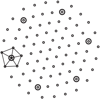
FIG. 8.: The magic number configuration $N=85$. Six five-coordinated particles associated with disclinations are marked by rings. Triangulation of the neighborhood of one of them is shown explicitly.

Let us define these defects. Elementary defect in a 2D lattice is disclination. The only possible form of such a defect in 2D crystals is the so-called wedge disclination. It can be viewed as a wedge which is removed (inserted) from the crystal. The “charge” of the disclination is the angle, formed by the wedge. The minimum possible disclination charge for a triangular lattice is $\pi/3$. The disclinations can be identified with the particles having an anomalous coordination number. In the triangular crystal the cores of the positive or negative disclinations are associated with the particles having five or seven nearest neighbors respectively, the normal coordination being six. Some examples of such defects are shown in Fig. 8.

Dislocations are the pairs of positive and negative disclinations forming a dipole. They can be seen in Fig. 9. When number of electrons in the island is less than some critical value $\tilde{N}\approx 150$, there exist highly symmetric electron configurations free of dislocations. These configurations can be realized only at some distinct values of $N=N_{m}=7,19,35,55,85$, which we call magic numbers. One of such magic number configurations $N_{m}=85$ is demonstrated in Fig. 8. On the other hand if $N>\tilde{N}$ the dislocations are always present and the magic number configurations never exist.

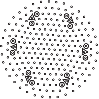
FIG. 9.: The electron configuration for $N=235$. The particles having five and seven nearest neighbors are shown by the rings and the triangles respectively.

We would like to stress again that all these defects are not observed directly on the surface. Moreover, if the number of electrons in the island is large, they do not come close to the surface. The same is true about the central region of the island. It is also usually free of defects. All the irregularities in the lattice are normally observed in a ring of width $(2\div 3)a$ at a fixed distance from the edge.

We would like to discuss now the accuracy of the results we have obtained. We believe that the total energy for the cases shown in Fig. 7a is calculated with precision $10^{-6}(e^{2}/\kappa)^{2/3}A^{11/3}$. This was tested by reruns (starting from different initial conditions) and comparison with the results of simulated annealing. The configurations however cannot be reproduced reliably. The thing is that several completely different configurations for the same number of electron can have very close energies, within $10^{-6}(e^{2}/\kappa)^{2/3}A^{11/3}$ from each other. However the general features of all these low energy configurations described above remain true. Thus, although we cannot reproduce the position of every individual defect reliably, we believe that we can say that in general defects reside in a ring concentric to the surface of the width of a few lattice constants.

We will see in Section VI that the interaction of defects is crucial in understanding of the energy fluctuations. In the next section we discuss the general properties of the defect distributions. These properties are essential for the arguments given in Section VI.

V Lattice Defects in the Circular Wigner Crystal Island

When the triangular crystal is packed into the island of circular form the obvious incompatibility of these two structures leads to the appearance of the lattice defects: disclinations and dislocations. The important difference between the former and the latter is that disclinations are always present in the ground state. The number of disclinations in the island is determined by the Euler’s theorem (see below) and, hence, cannot be changed. Dislocations on the other hand may or may not appear depending on whether they are energetically favorable. Let us first explain why the disclinations have to appear in the ground state.

The disclinations within some region of lattice can be identified by the number of $\pi/3$ turns that one has to make to walk around it. Normally one has to make minimum six such turns (consider for example the central point in Fig. 8). For the region having $N_{c}$ such defects inside, the minimum number of $\pi/3$ turns is $6-N_{c}$. Look e.g. at the pentagon in Fig. 8. It obviously contains one disclination, because the number of the aforementioned turns is five. Let us now mentally walk around the whole circular sample along its edge. As the surface of the island is circular we do not make any turns at all. Hence the total number of $\pi/3$ disclinations is exactly six:

$$N_{c}=6.$$ (49)

In the simplest possible case shown in Fig. 8 there are only six disclinations in the sample. If both positive (removal of $\pi/3$ wedge) and negative (insertion of such a wedge) disclinations are present, the total disclination charge should be calculated accounting for the sign of these defects:

$$N_{c}\equiv N_{c}^{+}-N_{c}^{-},$$ (50)

where $N_{c}^{+}$ and $N_{c}^{-}$ are the numbers of positive and negative defects correspondingly. Such complex cases are realized for example when there are a few dislocations in the island. Dislocation is a pair of positive and negative disclinations bound together to form a dipole. Hence addition of a dislocation to the sample increases both $N_{c}^{+}$ and $N_{c}^{-}$ keeping their difference the same. Consequently the number of dislocations is not controlled by the topological constraints expressed by Eq. (49). This equation can also be proved using Euler’s theorem. The proof can be found in Appendix  A.

Now let us turn to the dislocations. At zero temperature they embody inelastic deformations. There are two main reasons for existence of such deformations: inhomogeneity of the concentration of electrons and the presence of disclinations. The first reason is not universal: the exact profile of density is determined by the form of confinement and interaction potential. The second one is universal, because the presence of disclinations is required by theorem (49).

The dislocations produced by the varying crystal density were recently discussed by Nazarov. [13] He noticed that the dislocation density must be equal to the gradient of the reciprocal lattice constant:

$$\mathchoice{{\hbox{\boldmath$\displaystyle b$}}}{{\hbox{\boldmath$\textstyle b$}}}{{\hbox{\boldmath$\scriptstyle b$}}}{{\hbox{\boldmath$\scriptscriptstyle b$}}}\left(\mathchoice{{\hbox{\boldmath$\displaystyle r$}}}{{\hbox{\boldmath$\textstyle r$}}}{{\hbox{\boldmath$\scriptstyle r$}}}{{\hbox{\boldmath$\scriptscriptstyle r$}}}\right)=a\left(\mathchoice{{\hbox{\boldmath$\displaystyle r$}}}{{\hbox{\boldmath$\textstyle r$}}}{{\hbox{\boldmath$\scriptstyle r$}}}{{\hbox{\boldmath$\scriptscriptstyle r$}}}\right)\mathchoice{{\hbox{\boldmath$\displaystyle\hat{z}$}}}{{\hbox{\boldmath$\textstyle\hat{z}$}}}{{\hbox{\boldmath$\scriptstyle\hat{z}$}}}{{\hbox{\boldmath$\scriptscriptstyle\hat{z}$}}}\times\mathchoice{{\hbox{\boldmath$\displaystyle\nabla$}}}{{\hbox{\boldmath$\textstyle\nabla$}}}{{\hbox{\boldmath$\scriptstyle\nabla$}}}{{\hbox{\boldmath$\scriptscriptstyle\nabla$}}}a^{-1}\left(\mathchoice{{\hbox{\boldmath$\displaystyle r$}}}{{\hbox{\boldmath$\textstyle r$}}}{{\hbox{\boldmath$\scriptstyle r$}}}{{\hbox{\boldmath$\scriptscriptstyle r$}}}\right).$$ (51)

Here $\mathchoice{{\hbox{\boldmath$\displaystyle b$}}}{{\hbox{\boldmath$\textstyle b$}}}{{\hbox{\boldmath$\scriptstyle b$}}}{{\hbox{\boldmath$\scriptscriptstyle b$}}}\left(\mathchoice{{\hbox{\boldmath$\displaystyle r$}}}{{\hbox{\boldmath$\textstyle r$}}}{{\hbox{\boldmath$\scriptstyle r$}}}{{\hbox{\boldmath$\scriptscriptstyle r$}}}\right)$ is the density of Burgers vector, $\textstyle\hat{z}$ is the unit vector perpendicular to the surface, and $a=\sqrt{2/n\left(\mathchoice{{\hbox{\boldmath$\displaystyle r$}}}{{\hbox{\boldmath$\textstyle r$}}}{{\hbox{\boldmath$\scriptstyle r$}}}{{\hbox{\boldmath$\scriptscriptstyle r$}}}\right)\sqrt{3}}$ is the varying in space lattice constant. This formula is easy to understand. First we notice that a dislocation adds an extra row to the lattice. Hence the density of dislocations is given by the rate of change of concentration of these planes equal to $1/a$. To obtain the Burgers vector density we multiply this gradient by the elementary Burgers vector $a$ (see also Ref. [14]).

This formula has an interesting implication for the question of applicability of the elasticity theory to the Wigner crystal. Consider a sample of size $L$. Assume that there is a variation of concentration in the sample induced by an external source $\delta n\sim u_{ik}n$, where $u_{ik}$ is the strain tensor. Let us find the value of $u_{ik}$ at which dislocations start to appear. This would imply that inelastic (plastic) deformations occur and the elasticity theory brakes down. The energy of purely elastic deformations is

$$E_{\rm el}\sim YL^{2}u_{ik}^{2}.$$ (52)

Here $Y$ is the Young’s modulus. For inelastic deformations we have

$$E_{\rm inel}=E_{c}N_{d},$$ (53)

where $E_{c}$ is the dislocation core energy and $N_{d}$ is the total number of dislocations in the sample. Eq. (51) provides the following estimate for the latter:

$$N_{d}\sim L^{2}\frac{\delta n}{nLa}\sim u_{ik}\frac{L}{a}.$$ (54)

Comparing the elastic and inelastic energies we conclude that the deformations are completely elastic when

$$u_{ik}\lesssim\frac{E_{c}}{YaL}.$$ (55)

For the Wigner crystal with the Coulomb interaction using $E_{c}\sim e^{2}/\kappa a$, $Y\sim e^{2}/\kappa a^{3}$, and $u_{ik}\sim u/L$, where $u$ is the characteristic displacement, we obtain

$$u\lesssim a.$$ (56)

Hence equilibrium elastic displacements cannot exceed the lattice spacing for the Wigner crystal. This agrees with the known result that the elasticity theory has a zero radius of convergence with respect to the strain tensor. [15] In effect we conclude that the radius of convergence depends on the spacial scale of the problem and in the macroscopic limit $L\rightarrow\infty$ is indeed zero, according to (55). This surprising result emphasizes the difference between electron crystal and crystal consisting of heavy particles (atoms). In an electron crystal the relaxation time provided by tunneling is smaller than the time of experiment and, hence, the system can find the ground state. In an atomic crystal the relaxation time is typically much larger than the experimental time and the system can remain in the metastable state described by the elasticity theory.

Below we compare the number of dislocations of two different origin. First we calculate the total number of dislocations produced by the non-uniformity of the electron density. We consider the case of the Coulomb interaction. For this case the corresponding electrostatic problem (ignoring the discreteness of the charge of electrons) can be solved exactly. [16] The solution for the density of electrons can be shown to be a “hemisphere”:

$$\begin{array}[]{l}{\displaystyle n\left(r\right)=n_{0}\sqrt{1-\frac{r^{2}}{R^{2}}}}\\ \\ {\displaystyle n_{0}=\frac{4A\kappa R}{\pi^{2}e^{2}},~{}R=\left(\frac{3\pi Ne^{2}}{8A\kappa}\right)^{1/3}.}\end{array}$$ (57)

According to Eq. (51) the density of dislocations induced by varying electron density is

$$n_{d}(r)=\frac{b_{\phi}(r)}{h}=\sqrt{\frac{2n_{0}}{\sqrt{3}}}\frac{r}{R^{2}\left(1-r^{2}/R^{2}\right)^{3/4}}$$ (58)

Here $h=a\sqrt{3}/2$ is the elementary Burgers vector, equal to the distance between crystalline rows. The total number of dislocations is readily obtained by integrating this distribution:

$$N_{d1}=\int_{0}^{R}2\pi rdrn_{d}(r)\approx 4.08\cdot N^{1/2}.$$ (59)

The electrostatic formula (57) is correct if the number of electrons is large. In the opposite case of a small island the density profile is very far from being a hemisphere. In this case the density is almost constant.[5] This is obvious from looking at Figs. 8 and 9 above. To evaluate the variation of the electron density we will find the lattice constant on the surface of the island and compare it to that in the center. To this end we notice that near the edge the density of dislocations given by Eq. (58) would become infinitely large. However it cannot exceed the density of electron themselves, given by Eq. (57). The position of the edge of the crystal can therefore be determined matching the dislocation density and the density of electrons. As a result we obtain for the lattice constant on the edge the following expression:

$$\lambda\sim a_{0}^{4/5}R^{1/5}\propto N^{-1/15}.$$ (60)

This expression agrees with conclusions of Ref. [5] obtained in a different way. Our numerical data agree very well with this theory and give the following coefficient:

$$\begin{array}[]{c}{\lambda=0.88a_{0}^{4/5}R^{1/5},}\end{array}$$ (61)

The interelectron distance on the edge given by this formula differs very slightly from the lattice constant in the center of the sample if the radius of the island is not too large. To evaluate the number of dislocations for a small island we approximate the electron density profile with a parabola:

$$n(r)\simeq n_{0}\left[1-\frac{r^{2}}{R^{2}}\left(1-\frac{a_{0}^{2}}{\lambda^{2}}\right)\right].$$ (62)

Applying Eq. (51) to this expression we obtain

$$N_{d1}\approx 2.05\cdot N^{1/2}\left(1-\frac{a_{0}^{2}}{\lambda^{2}}\right)$$ (63)

In the consideration below we will assume that the number of electrons in the island is not too large. Therefore the electron density is almost uniform.

As it was mentioned above, another reason for appearance of dislocations is the stress, produced by disclinations. The latter deform the lattice enormously. These deformations can be significantly reduced by introducing dislocations into the lattice. This process is usually referred to as screening. The screening of disclinations by dislocations has been studied before in the context of the hexatic liquid – homogeneous liquid transition.[18] The screening is that case is accomplished by polarization of the thermally excited dislocations above the Kosterlitz-Thouless transition. It was therefore treated in the framework of the linear Debye-Huckel approximation. Here we deal with the case when there are no thermally excited dislocations and all the Burgers vector density necessary for screening exists due to the appearance of new dislocations.

The phenomenon can be most easily understood considering the total disclination density: [18]

$$s_{\rm tot}(\mathchoice{{\hbox{\boldmath$\displaystyle r$}}}{{\hbox{\boldmath$\textstyle r$}}}{{\hbox{\boldmath$\scriptstyle r$}}}{{\hbox{\boldmath$\scriptscriptstyle r$}}})=s(\mathchoice{{\hbox{\boldmath$\displaystyle r$}}}{{\hbox{\boldmath$\textstyle r$}}}{{\hbox{\boldmath$\scriptstyle r$}}}{{\hbox{\boldmath$\scriptscriptstyle r$}}})-\varepsilon_{ik}\nabla_{i}b_{k}(\mathchoice{{\hbox{\boldmath$\displaystyle r$}}}{{\hbox{\boldmath$\textstyle r$}}}{{\hbox{\boldmath$\scriptstyle r$}}}{{\hbox{\boldmath$\scriptscriptstyle r$}}}),$$ (64)

where the first term is the density of free disclinations while the second is the density of disclinations induced by the varying in space density of dislocations (the latter are the dipoles formed from the former). The elastic energy of the crystal can be written in terms of this total defect density:

$$E=\frac{Y}{2}\int\frac{d^{2}q}{(2\pi)^{2}}\frac{\left|s_{\rm tot}(\mathchoice{{\hbox{\boldmath$\displaystyle q$}}}{{\hbox{\boldmath$\textstyle q$}}}{{\hbox{\boldmath$\scriptstyle q$}}}{{\hbox{\boldmath$\scriptscriptstyle q$}}})\right|^{2}}{q^{4}},$$ (65)

where $Y$ is the Young’s modulus. For case of the Coulomb crystal [19] $Y=\alpha e^{2}n^{3/2}/\kappa$, where $\alpha=0.9804$. We notice that for the large distances $q\rightarrow 0$ the numerator in this expression is pushed to zero by the $q^{4}$ term contained in the denominator. Thus, ignoring the effects at the distances $r\sim a$, one can write the condition of the perfect screening:

$$s_{\rm tot}(\mathchoice{{\hbox{\boldmath$\displaystyle r$}}}{{\hbox{\boldmath$\textstyle r$}}}{{\hbox{\boldmath$\scriptstyle r$}}}{{\hbox{\boldmath$\scriptscriptstyle r$}}})=0.$$ (66)

It is instructive now to consider one disclination in the center of an infinite sample: $s(\mathchoice{{\hbox{\boldmath$\displaystyle r$}}}{{\hbox{\boldmath$\textstyle r$}}}{{\hbox{\boldmath$\scriptstyle r$}}}{{\hbox{\boldmath$\scriptscriptstyle r$}}})=s_{0}\delta(\mathchoice{{\hbox{\boldmath$\displaystyle r$}}}{{\hbox{\boldmath$\textstyle r$}}}{{\hbox{\boldmath$\scriptstyle r$}}}{{\hbox{\boldmath$\scriptscriptstyle r$}}})$. Equations (66) and (64) have in general many solutions. Two of them are easy to guess: $b_{1\phi}=s_{0}/2\pi r$, $b_{1r}=0$ and $b_{2x}=0$, $b_{2y}=s_{0}\Theta(x)\delta(y)$. They represent the Burgers vector rotating around the disclination and the solution in the form of a grain boundary respectively. They are different by the longitudinal Burgers vector density: $\mathchoice{{\hbox{\boldmath$\displaystyle b_{1}$}}}{{\hbox{\boldmath$\textstyle b_{1}$}}}{{\hbox{\boldmath$\scriptstyle b_{1}$}}}{{\hbox{\boldmath$\scriptscriptstyle b_{1}$}}}=\mathchoice{{\hbox{\boldmath$\displaystyle b_{2}$}}}{{\hbox{\boldmath$\textstyle b_{2}$}}}{{\hbox{\boldmath$\scriptstyle b_{2}$}}}{{\hbox{\boldmath$\scriptscriptstyle b_{2}$}}}+\nabla f$, where $f$ is some scalar function, and hence have the same elastic energy. This non-uniqueness is a consequence of essentially mean-field character of Eq. (66). Discreteness of the dislocations removes this degeneracy in favor of the grain boundary. The idea is that the fluctuations of the local elastic energy caused by the discreteness of the defects can be estimated as $E\sim Ya^{2}\ln(\left<r\right>/a)$ per defect, where $\left<r\right>$ is the average distance between them. In the former distribution $\textstyle b_{1}$ this average distance grows with the size of the sample $\left<r\right>\sim\sqrt{La}$. In the case of the grain boundary the average distance is maintained of the order of the lattice spacing. Hence the self-energy of defects in the latter case does not grow with the size of the sample.

The next logical step is to consider six disclinations in the circular crystalline sample. A possible solution for the distribution of defects is shown in Fig. 10. It is prompted by the results of the numerical simulations showing that in the majority of cases the defects (dislocations and disclinations) are situated in a ring concentric to the surface of the island. The regions adjacent to the center and to the edge of the island appear to be free of defects. We assume that the disclinations form a figure close to a perfect hexagon. The dislocations form grain boundaries connecting the disclinations. This is done to smear out the charge of disclinations in accordance with the screening theory expressed by Eq. (66).

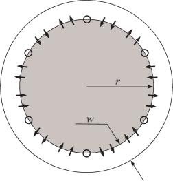
FIG. 10.: The distribution of defects in a compressible island. Rings and arrows show the positions of disclinations and the direction of the Burgers vector density, respectively. The gray disk shows the free of defects central region.

Next we calculate the distance from the surface to the layer of defects. We consider the case of a uniform crystal. The central region of the island can be formed with no deformations in it. It can be thought of as a piece of the uniform crystal having a circular form, the same as the one considered in Sections II and III. The central region is shown in Fig. 10 by a gray disk. The region between the surface of the island and the layer of defects is free of defects too. It cannot be free of elastic deformations however. These deformations are the same as those of a 2D rectangular elastic rod, two opposite edges of which are glued together. To find the optimum thickness of this rod $w$ (see Fig. 10) one has to balance the energy associated with this bending, which tends to reduce $w$, and the surface energy of the grain boundary. The latter is proportional to the length of the grain boundary and therefore has a tendency to increase $w$. The bending energy can be calculated from the elasticity theory [20]

$$E_{\rm el}=\frac{\pi}{12}Y\frac{w^{3}}{R}.$$ (67)

The surface energy of the grain boundary can be estimated from the core energies of the dislocations:

$$E_{\rm gb}\approx E_{c}N_{d}$$ (68)

The total number of dislocation follows from elementary geometric calculation done for the incompressible crystalline region of radius $r=R-w$:

$$N_{d2}=12(1-\sqrt{3}/2)r/h,$$ (69)

where $h=a\sqrt{3}/2$. Minimizing the total energy $E=E_{\rm el}+E_{\rm gb}$ we find the optimum at:

$$w\approx 1.5\sqrt{\frac{E_{c}R}{Ya}}\approx 0.5\sqrt{Ra}.$$ (70)

In the derivations of (70) we used $E_{c}=0.11e^{2}n^{1/2}/\kappa$ and $Y=0.9804e^{2}n^{3/2}/\kappa$ (Ref. [19]). This result can be also obtained from our condition of stability of a crystal (56). Indeed the strain tensor in the ring can be estimated as $u_{\phi\phi}\sim w/R$. The corresponding displacement $u\sim w^{2}/R$ cannot exceed the lattice spacing $a$, according to Eq. (56). The estimate for the width of the ring $w$ obtained from this argument is consistent with Eq. (70).

Now we would like to find the condition at which the dislocations stay on the surface of the island. We will consider the case of the short-range interaction (4). To this end one has to compare the energy of the defects on the boundary with that in the bulk of the crystal. The former is associated with the roughness of the surface (see Fig. 1). It can be estimated as a product of the total number of particles there $\sqrt{N}$, the typical force acting on a particle on the surface $F(R)=2AR$, and the characteristic deviation of the shape of the surface from the circle, given by the lattice constant: $\delta E_{\rm sur}\sim\sqrt{N}\cdot F(R)\cdot a$. The energy of the defects inside the island is given by $\delta E_{\rm bulk}\sim\sqrt{N}\cdot Ya^{2}\ln N$. The first term in the right-hand side is the number of defects and the second one is the typical energy per dislocation. It is estimated as the typical interaction energy of two dislocations. Note that we neglect the core energy of dislocations as it is small compared to the $Ya^{2}$ for the crystal with short-range interaction. Indeed the former is of the order of the correlation energy: $E_{c}\sim U_{0}\exp(-a/s)$. The Young’s modulus for the considered system can be estimated as the second derivative of the interaction potential between two particles:

$$Y\sim\frac{U_{0}}{s^{2}}\exp\left(-\frac{a}{s}\right).$$ (71)

It is clear then that $E_{c}/Ya^{2}\sim s^{2}/a^{2}\ll 1$. Comparison of $\delta E_{\rm sur}$ with $\delta E_{\rm bulk}$ gives the condition that the defects stay on the surface:

$$Y\ln N\gg A\sqrt{N}.$$ (72)

The coefficient $A$ can be conveniently related to the interaction strength by balancing the forces acting on a particle on the surface: $AR\sim U_{0}/s\cdot\exp(-a/s)$. Combining this equation with Eq. (71) and (72) we obtain the following condition for the defects staying on the boundary:

$$a\ln N\gg s$$ (73)

This coincides with the condition of uniformity of the crystal (see Section III). Note that this entire consideration is based on the assumption of uniformity of the crystal.

Finally in this section we evaluate the critical number of electrons $N^{*}$ at which the number of dislocations due to the inhomogeneity of the electron density $N_{d1}$ and produced by the screening of disclinations $N_{d2}$ become equal. To do so we compare Eq. (63) with Eq. (69). They become equal if $\lambda\approx 1.55a_{0}$ or, using Eq. (60)

$$N=N^{*}\simeq 700.$$ (74)

Therefore if the number of electrons in the island is smaller that $N^{*}$ we dislocations are mostly due to the screening of disclinations and are arranged into the grain boundary (see Fig. 10). In the opposite case the dislocations are generated in the interior according to Eq. (51).

The above consideration is essentially mean-field, treating the density of dislocations as a continuous quantity. In the next section we give an argument that the discreteness of dislocations is responsible for the fluctuations of the elastic energy of the Wigner lattice.

VI Elastic Blockade

The number of dislocations in the Wigner crystal island is of the order of the number of crystalline rows in it [see Eq. (69)]:

$$N_{d}\sim R/a\sim\sqrt{N}.$$ (75)

Hence, it grows while the island in filled with electrons. On the average one dislocation appears as $N$ increases by $\delta N\sim\sqrt{N}$. The elastic energy stored due to the deviation of the number of dislocations from the average is relaxed when a new one is added. This phenomenon is similar to the Coulomb blockade, with the words “electron” and “electrostatic energy” replaced by “dislocation” and “elastic energy”.

Using this analogy to the Coulomb blockade one can easily estimate the order of the fluctuations of energy. In the Coulomb blockade case the fluctuations of the electrostatic energy are given by the following expression:

$$\delta E=\frac{e^{2}}{2C}\delta N^{2},$$ (76)

where $-1/2\leq\delta N<1/2$ is the deviation of the number of electrons in the dot from the average, determined by the gate voltage. Following the convention of the above mapping one has to replace $e^{2}/C$ by the characteristic energy of interaction of two dislocations in the island $U_{0}\sim Ya^{2}\sim e^{2}/\kappa a$. One also has to replace $\delta N$ by the deviation of the number of dislocations from the average $\delta N_{d}\sim\delta N/\sqrt{N}$. As a result we obtain:

$$\delta E_{\rm el}=\alpha\frac{e^{2}}{\kappa a}\frac{\delta N^{2}}{N}.$$ (77)

Here $\alpha\approx 0.5$ is a numerical constant. The approximate value of this constant is obtained from the numerical results of Section IV. As the total period of such an “elastic” blockade is $T_{N}\sim\sqrt{N}$, the maximum fluctuation of energy that can be reached is $\delta E_{\rm max}\sim\alpha e^{2}/\kappa a$.

Another implication of this analogy is the appearance of the elastic blockade peaks. In the case of Coulomb blockade the intersection of two terms described by Eq. (76) for different numbers of electrons in the dot produce a spike in the conductance through the dot. At this point a new electron enters the dot. For the “elastic” blockade at the similar point a new dislocation enters the crystalline island. The chemical potential of an electron has a discontinuity of the order of $\Delta\mu\sim dE/dN\sim-\alpha e^{2}/\kappa aT_{N}\sim-\alpha e^{2}/R$. The charging energy at this point fluctuates by a value

$$\delta\Delta=\frac{d\delta\mu}{dN}=\frac{\Delta\mu}{1}\sim-\alpha\frac{e^{2}}{\kappa R},$$ (78)

which is of the order of the average $\overline{\Delta}=\beta e^{2}/\kappa R$, $\beta$ being another constant. This however does not lead to the bunching in the charging spectrum as it did in the case of the short-range interaction, because of the smallness of the numerical constant $\alpha$.

Let us consider the elastic blockade in more detail. In the previous section we derived the condition at which the crystal can be considered to be uniform. If the number of electrons in the island is less than some critical value $N^{*}\simeq 700$, the variations in the density of electrons can be ignored and the number of dislocations associated with the variable density is small. Below we examine these two regimes separately.

i) Almost uniform crystal: $N\lesssim N^{*}$.

As it follows from the previous section in this regime the density of electrons in the island is almost uniform. The crystal is packed into the circular form by forming two monocrystals: the almost circular internal region, free of elastic deformations, similar to the incompressible island; and the external ring (see Fig. 10). The interface between these two monocrystals is a grain boundary, which can be viewed as a string of dislocations.

Assume now that the position of the center of the confinement relative to the lattice $\mathchoice{{\hbox{\boldmath$\displaystyle r$}}}{{\hbox{\boldmath$\textstyle r$}}}{{\hbox{\boldmath$\scriptstyle r$}}}{{\hbox{\boldmath$\scriptscriptstyle r$}}}_{0}$ is fixed. This coordinate has been introduced earlier in Section III. One can then calculate the energy of the island as a function of the number of electrons and the position of the center $E_{\mathchoice{{\hbox{\boldmath$\displaystyle r$}}}{{\hbox{\boldmath$\textstyle r$}}}{{\hbox{\boldmath$\scriptstyle r$}}}{{\hbox{\boldmath$\scriptscriptstyle r$}}}_{0}}(N)$. Due to the symmetry considerations given in Section III this function has extrema at the point A, B, and C shown in Fig. 6a similar to the incompressible island. Filling of the island results in switching among three energetic branches $E_{A}(N)$, $E_{B}(N)$, and $E_{C}(N)$, every time choosing the lowest. Below in this subsection we estimate the correction to the total energy $\delta E_{\mathchoice{{\hbox{\boldmath$\displaystyle r$}}}{{\hbox{\boldmath$\textstyle r$}}}{{\hbox{\boldmath$\scriptstyle r$}}}{{\hbox{\boldmath$\scriptscriptstyle r$}}}_{0}}(N)$.

The grain boundary has a tendency to be at a fixed distance from the center $r=R-w$, calculated in Section V. If position of the center relative to the crystal is fixed, filling of the island brings about expanding of the mean grain boundary position with respect to the crystal. Hence, periodically the grain boundary has to intersect a new crystalline row. At this moment in the corresponding incompressible problem a new terrace appears on the boundary of the island. In the Coulomb problem the grain boundary is submerged into the island. Therefore at this moment in the compressible case a new row is added to the island. Since the termination points of the new row can be thought of as dislocations, we can say that a new pair of opposite dislocations appears on the grain boundary (see Fig. 10 with the gray internal region shown in more detail in Fig. 3).

The corresponding fluctuation of energy can be evaluated as the energy of interaction of two opposite dislocations having charge $\delta N_{d}=N_{d}-\overline{N}_{d}$, where $N_{d}$ is the actual number of dislocations in the neighborhood of the new row, $\overline{N}_{d}$ is the average one. This energy is given by:[18]

$$\delta E_{0}\simeq\frac{Yh^{2}}{4\pi}\delta N_{d}^{2}\ln\left(\frac{l}{h}\right).$$ (79)

The typical distance between defects $l$ is given by Eq. (25): $l\sim\sqrt{R\cdot a}$. The average number of dislocations is given by the number of crystalline rows $\overline{N}_{d}=\sum_{i}(r-\mathchoice{{\hbox{\boldmath$\displaystyle\hat{e}$}}}{{\hbox{\boldmath$\textstyle\hat{e}$}}}{{\hbox{\boldmath$\scriptstyle\hat{e}$}}}{{\hbox{\boldmath$\scriptscriptstyle\hat{e}$}}}_{i}\mathchoice{{\hbox{\boldmath$\displaystyle r$}}}{{\hbox{\boldmath$\textstyle r$}}}{{\hbox{\boldmath$\scriptstyle r$}}}{{\hbox{\boldmath$\scriptscriptstyle r$}}}_{0})/h$, $\mathchoice{{\hbox{\boldmath$\displaystyle\hat{e}$}}}{{\hbox{\boldmath$\textstyle\hat{e}$}}}{{\hbox{\boldmath$\scriptstyle\hat{e}$}}}{{\hbox{\boldmath$\scriptscriptstyle\hat{e}$}}}_{i}$ being the unit vector normal to the series of rows considered. Therefore

$$\delta N_{d}=\sum_{i=1}^{6}\left\{\frac{r-\mathchoice{{\hbox{\boldmath$\displaystyle\hat{e}$}}}{{\hbox{\boldmath$\textstyle\hat{e}$}}}{{\hbox{\boldmath$\scriptstyle\hat{e}$}}}{{\hbox{\boldmath$\scriptscriptstyle\hat{e}$}}}_{i}\mathchoice{{\hbox{\boldmath$\displaystyle r$}}}{{\hbox{\boldmath$\textstyle r$}}}{{\hbox{\boldmath$\scriptstyle r$}}}{{\hbox{\boldmath$\scriptscriptstyle r$}}}_{0}}{h}\right\}-\frac{1}{2},$$ (80)

where by $\{\cdots\}$ we assume taking the fractional part. The oscillations of energy are given by the formula similar to Eq. (44)

$$\delta E_{\mathchoice{{\hbox{\boldmath$\displaystyle r$}}}{{\hbox{\boldmath$\textstyle r$}}}{{\hbox{\boldmath$\scriptstyle r$}}}{{\hbox{\boldmath$\scriptscriptstyle r$}}}_{0}}=\sum_{i=1}^{6}\delta E_{0}(r-\mathchoice{{\hbox{\boldmath$\displaystyle\hat{e}$}}}{{\hbox{\boldmath$\textstyle\hat{e}$}}}{{\hbox{\boldmath$\scriptstyle\hat{e}$}}}{{\hbox{\boldmath$\scriptscriptstyle\hat{e}$}}}_{i}\mathchoice{{\hbox{\boldmath$\displaystyle r$}}}{{\hbox{\boldmath$\textstyle r$}}}{{\hbox{\boldmath$\scriptstyle r$}}}{{\hbox{\boldmath$\scriptscriptstyle r$}}}_{0}),$$ (81)

where

$$\delta E_{0}(r)\simeq\frac{Yh^{2}}{16\pi}\left[\left(\left\{\frac{r}{h}\right\}-\frac{1}{2}\right)^{2}-\frac{1}{12}\right]\ln N$$ (82)

are the fluctuations of energy given by (79). The last term in the square brackets is chosen so that $\overline{\delta E_{0}(r)}=0$.

The oscillations of energy calculated in this way for three positions of the center $\mathchoice{{\hbox{\boldmath$\displaystyle r$}}}{{\hbox{\boldmath$\textstyle r$}}}{{\hbox{\boldmath$\scriptstyle r$}}}{{\hbox{\boldmath$\scriptscriptstyle r$}}}_{0}=$ A, B, and C are shown in Fig. 11.

FIG. 11.: The fluctuating part of the energy of the Wigner crystal island calculated from the interaction of dislocations.

As usually the lowest one is to be chosen. Comparison to the numerical experiment (Fig. 7) shows, that this model predicts very well the phase and the shape of the oscillations. The amplitude however is smaller by a factor of $2\div 2.5$ than observed in the simulations. This difference can be explained by the influence of the boundary of the sample on the interaction energy of dislocations (79). Indeed the boundary of the island is at the distance $w\approx 0.5\sqrt{R\cdot a}$ from the ring of dislocations. This scale is smaller than the characteristic distance between dislocations $l\approx(2\div 3)\sqrt{R\cdot a}$. Hence the boundary of the island should play an important role in the interaction of dislocations.

To understand the character of the correction we notice that the boundary in the numerical experiment is almost not deformed. The island tends to preserve its circular shape. Hence we can assume that the normal displacement of the boundary is zero. Assume now that the dislocations are much farther away from each other than from the boundary $l\gg w$. In practice we have $l\approx 5w$. The problem of interaction of the pair of dislocations in the presence of the boundary can then be solved using the method of images. It is easy to see that at the zero normal displacement boundary condition a dislocation with the Burgers vector perpendicular to the boundary produces an image of the same sign. Indeed such a dislocation is a crystalline semi-row, parallel to the surface. The zero normal displacement boundary condition can be realized by putting a parallel semi-row on the other side of the boundary. Hence effectively the boundary doubles the charge of each dislocation. The interaction energy, being proportional to the square of charge, would acquire a factor of four due to such images. However as the crystal exists only in the semi-space the deformations only there contribute to the elastic energy. Therefore the overall factor that arises due to the presence of the boundary is $4\cdot 1/2=2$:

$$E_{\rm boundary}(r)=2E_{\rm free}(r)=\frac{Yh^{2}}{2\pi}\ln\left(\frac{r}{a}\right).$$ (83)

This factor can explain the discrepancy between our calculation and the numerical experiment.

ii) Non-uniform crystal: $N\gg N^{*}$.

In this case as it follows from Eq. (58) there are $N_{d}\sim\sqrt{N}$ dislocations in the island associated with the variations of the electron density. According to Eq. (58) these defects have to be present in the bulk of the crystal. Hence they cannot be arranged into grain boundaries as in the case considered above. The nearest dislocations repel each other and one could imagine that they form a crystal themselves. [13] We argue however that this cannot be the case. The reason is that dislocation can occupy a fixed position within an electron lattice cell. Hence the incommensurability of the electron and dislocation lattices eventually produces frustration and destroys the long-range order in the dislocation lattice. Therefore we expect that the dislocations form a glassy state.

This implies that the coherence of the crystalline rows in the electron crystal itself is destroyed. We think therefore that in this regime the variations of the total energy are not periodic. They retain however the general features described in the introduction to this section. To understand how these features arise in this particular case we would like to study the reconstructions in the dislocation lattice caused by addition of a new electron. To this end it is necessary to consider two cases: when this addition does not change the total number of defects, and when the number of defects is increased. The former case takes place most of the time, while the latter happens once in $\sqrt{N}$ electrons when a new defect has to appear.

Consider the first case. Electron can be added into the core of dislocation increasing the length of the extra crystalline row associated with it. The dislocation after this is displaced by the lattice constant. Let us find the maximum change in the elastic energy of the island associated with such a displacement. It can be expressed through the interaction between dislocations:

$$\delta E_{\rm max}\sim\frac{d^{2}U(r)}{dr^{2}}a^{2},$$ (84)

where $U(r)=Yh^{2}\ln(r)/4\pi$ is the dislocation interaction energy. The reason why the second derivative is relevant to the calculation of this energy is that the dislocation is in equilibrium before adding the new electron. Hence the gradient of the self-energy of the dislocation is zero. Now we have to remember that there are $\sqrt{N}$ dislocations in the island. Hence the actual addition energies range from zero to $\delta E_{\rm max}$ with the average level spacing

$$\delta E\sim\frac{\delta E_{\rm max}}{\sqrt{N}}\sim\frac{e^{2}a}{\kappa R^{2}}.$$ (85)

This quantity describes the energy one pays when adding an electron at the fixed number of dislocations. This is a correction to the energy spacing. Multiplied by the total number of electrons between two consecutive additions of dislocations $\sqrt{N}$ it gives the variation of the chemical potential $\delta E\sqrt{N}\sim e^{2}/\kappa R$. This variation should be equal to the discontinuity of the chemical potential when a new dislocation is added to the island, as the average correction to this quantity due to elastic effects does not grow. Thus the drop of chemical potential is equal to $\delta\mu\sim e^{2}/\kappa R$. This is consistent with Eq. (78).

Thus elongated crystalline lines draw dislocations from the center to the periphery of the island. Eventually a new row has to be inserted in the center. This event manifests itself in the appearance of a new pair of dislocations. The distance from the center $\xi$ at which they are situated can be found from Eq. (58) by stating that

$$n_{d}(\xi)\sim\frac{1}{\xi^{2}}.$$ (86)

This results in

$$\xi\sim a^{1/3}R^{2/3}.$$ (87)

The energetics of switching between two branches corresponding to different number of dislocations has already been discussed above [see Eq. (78)].

VII Conclusions

In this section we would like to discuss the degree of universality of our results. The first question is what happens if confinement potential $V(r)$ is not parabolic. The answer is almost obvious for the hard-disc interaction. In this case electrons are added to the crystal on the equipotential determined by the level of chemical potential. Therefore only the shape of this equipotential and the confinement potential gradient matter for energy fluctuations. It is obvious that situation is almost identical for any isotropic confinement $V(r)$. It is also easy to generalize our calculations for the confinements of oval shapes.

In the latter case the theory developed in Section III can be applied with a few modifications. As it was explained the variations of energy are associated with periodic intersections of the equipotentials with the crystalline rows. The main contribution to these oscillations comes from the “coherence” spots of the size $\sim\sqrt{R\cdot a}$ tangential to the rows. The oscillations of energy are sensitive then only to the properties of the equipotential in the immediate vicinity to those spots. If it can be well approximated there by a circle Eq. (44) should hold with additional phase shifts introduced into the arguments of the contributions from different rows. These phase shifts arise due to the deviation of the global shape of the equipotential from the circle, and express the incoherence of contributions coming from six different series of rows. In addition to that each contribution should be rescaled according to $\delta\Omega_{0}\propto\sqrt{R_{i}}T_{\mu}$, where $R_{i}$ is the curvature radius of the corresponding equipotential. We would like to emphasize again that this theory works only for an island of oval shape. It is not applicable for example to a square. All of the curvature radii $R_{i}$ have to be of the order of the size of the island. In general as the contributions from different terraces are not coherent anymore, the overall amplitude of oscillations has to be smaller in the oval case compared to the case of rotational symmetry.

Let us discuss the universality of the results with respect to the choice of the interaction potential. As we have seen both short-range and Coulomb interactions give rise to the fluctuations of energy of the same functional shape. We argue that the other forms of long-range interactions, logarithmic for instance, bring about similar results. Thus the energy of a disorder-free cylinder or disk of a type-II superconductor filled with the fluxoid lattice or a rotating cylindrical vessel of the superfluid helium as a function of the number of vortices[21] should experience oscillations similar to those in Fig. 7. To check this prediction we have performed a numerical calculation in our model with the interaction $U(r)=U_{0}\ln(1/r)$. It revealed a quasi-periodic correction to the energy of the same functional shape as shown in Fig. 7. The amplitude of the correction was consistent with the conclusions of Section VI. The configurations were also very similar to the observed in the Coulomb case. In particular the correlation between the position of the center of the confinement relative to the crystal and the oscillations of the energy is also observed.

In conclusion we have studied the charging spectrum of the crystal formed by particles in the parabolic confinement. We considered two forms of the interactions between particles: the short-range and Coulomb interactions. In the computer simulations employing the genetic algorithm we have observed the oscillations of the ground state energy which have a universal form, independent of the form of interaction. We attribute these oscillations to the combination of two effects: periodic additions of new crystalline rows and hopping of the center of the confinement relative to the crystal. The hops are separated by addition of $\sim N^{1/2}$ electrons. These hops make a dramatic difference for the addition spectrum of the island. In the case of the short-range interaction they make the charging energy negative, so that $\sim N^{1/4}$ new electrons enter the island simultaneously. This apparent attraction between electrons is a result of the confinement polaron effect discussed in Ref. [5]. In the case of Coulomb interaction such a hop results in an abrupt $\approx 15\%$ decrease in the charging energy.

VIII Acknowledgements

We thank M. Fogler, A. I. Larkin, J. R. Morris, D. R. Nelson, and N. Zhitenev for stimulating discussions and numerous useful suggestions. This work is supported by NSF grant DMR-9616880.

A The Total Disclination Charge of The Island and the Euler’s Theorem

To prove Eq. (49) one has to first consider some triangulation of the electron lattice. It is convenient to consider the triangulation in which every electron is connected by edges to the nearest neighbors. In the case of triangular lattice an electron in the bulk has six nearest neighbors, while an electron on the surface of the sample has only four. For some electrons however this number can be different. For example, an electron in the core of $\pi/3$ disclination has only five nearest neighbors (see Fig. 8). Electrons on the surface can have the coordination number equal to three. We associate such electrons with the $\pi/3$ disclinations stuck to the surface.

Let us now use the Euler’s theorem. For our case it says:

$$v+f-e=1,$$ (A1)

where $v$, $f$, and $e$ are the numbers of vertices, faces, and edges contained in the graph formed by our triangulation. All the vertices of the graph can be divided into the internal ones $v_{i}$, belonging to the bulk, and the ones on the surface $v_{e}$. The same can be done for the edges:

$$\begin{array}[]{c}{v=v_{i}+v_{e}}\\ {e=e_{i}+e_{e}}.\end{array}$$ (A2)

As all the faces of our figure are triangular by construction the following relationship, expressing the general balance of edges, is true:

$$3f=e_{e}+2e_{i}.$$ (A3)

Next we can relate the number of edges to the number of vertices. As it was mentioned above the bulk vertices are connected to six edges while the surface ones to four. The exceptions are the cores of disclinations. They have an anomalous coordination number. Expressing now the overall balance of edges one can write:

$$2e=6v_{i}-\delta v_{i}+4v_{e}-\delta v_{e},$$ (A4)

where $\delta v_{i}$ and $\delta v_{e}$ are total deviations from the normal coordination numbers for the internal and external vertices respectively. One can finally use the obvious fact that

$$v_{e}=e_{e}$$ (A5)

to solve the system of equations (A1) - (A4) and to obtain:

$$N_{c}=\delta v_{i}+\delta v_{e}=6.$$ (A6)

This completes the proof of Eq. (49). We would like to notice that a similar theorem is well known for a triangular crystal on the surface of a sphere: [7, 22]

$$N_{c}=12.$$ (A7)

REFERENCES

- [1] N. B. Zhitenev, R. C. Ashoori, L. N. Pfeiffer, and K. W. West, preprint cond-mat/9703241 (1997).
- [2] R. C. Ashoori, H. L. Stormer, J. C. Weiner, L. N. Pfeiffer, K. W. Baldwin, S. J. Pearton, and K. W. West, Phys. Rev. Lett.68, 3088 (1992); R. C. Ashoori, H. L. Stormer, J. C. Weiner, L. N. Pfeiffer, K. W. Baldwin, and K. W. West, Phys. Rev. Lett.71, 613 (1993).
- [3] Y. Wan, G. Ortiz, and P. Phillips, Phys. Rev. Lett.75, 2879 (1995).
- [4] M. E. Raikh, L. I. Glazman, L. E. Zhukov, Phys. Rev. Lett., 77, 1354 (1996).
- [5] A. A. Koulakov, B. I. Shklovskii, preprint cond-mat/9705030 (1997).
- [6] V. M. Bedanov and F. M. Peeters, Phys. Rev. B49, 2667 (1994).
- [7] J. R. Morris, D. M. Deaven, K. M. Ho, Phys. Rev. B53, R1740 (1996).
- [8] L. D. Landau and E. M. Lifshitz, Elasticity Theory (Reed Educational and Professional Publishing Ltd, Exeter, 1996), Section 7, Problem 5.
- [9] P. M. Bleher, F. J. Dyson, and J. L. Lebowitz, Phys. Rev. Lett.71, 3047 (1993); P. M. Bleher, Z. Cheng, F. J. Dyson, and J. L. Lebowitz, Commun. Math. Phys. 154, 433 (1993).
- [10] E. T. Whittaker, G. N. Watson, A Course of Modern Analysis (Cambridge University Press, 1963), p. 265.
- [11] L. D. Landau and E. M. Lifshitz, Statistical Physics, Part 1 (Reed Educational and Professional Publishing Ltd, Exeter, 1996), Section 24.
- [12] For our case the theorem of small increments can be proved in the following way: . Now we use the identity to obtain
- [13] Y. V. Nazarov, Europhys. Let. 32, p 443-8 (1996); see also preprint cond-mat/9509133.
- [14] Eq. (51) is a consequence of a more general statement that the total density of disclinations is equal to the curvature tensor in the crystal (see R. de Wit, Int. J. Eng. Sci. 19, 1475 (1981)). For the deformations induced by the variable density of electrons it is true that , where is the density of disclinations, is the completely anti-symmetric tensor, and is the scalar curvature. Assuming no free disclinations , we obtain Eq. (51) for the transverse component of the Burgers vector density.
- [15] A. Buchel and J. P. Sethna, Phys. Rev. Lett.77, 1520 (1996).
- [16] Ian N. Sneddon, Mixed Boundary Value Problems in Potential Theory (John Wiley & Sons, Inc., New York, 1966).
- [17] A. L. Efros, Solid State Communications 65, 1281 (1988).
- [18] P. M. Chaikin, T. C. Lubensky, Principles of Condensed Matter Physics (Cambridge University Press, 1995).
- [19] D. S. Fisher, B. I. Halperin, and R. Morf, Phys. Rev. B20, 4692 (1979).
- [20] cf. Ref. [8], Section 11.
- [21] L. J. Campbell and R. M. Ziff, Phys. Rev. B20, 1886 (1979).
- [22] D. R. Nelson, Phys. Rev. B, 28, 5515 (1983); M. J. W. Dodgson and M. A. Moore preprint cond-mat/9512123.