Effect of Shear Flow on the Stability of Domains in Two Dimensional Phase-Separating Binary Fluids

Abstract

We perform a linear stability analysis of extended domains in phase-separating fluids of equal viscosity, in two dimensions. Using the coupled Cahn-Hilliard and Stokes equations, we derive analytically the stability eigenvalues for long wavelength fluctuations. In the quiescent state we find an unstable varicose mode which corresponds to an instability towards coarsening. This mode is stabilized when an external shear flow is imposed on the fluid. The effect of the shear is seen to be qualitatively similar to that found in experiments.

I Introduction

Phase separating binary fluids form complex patterns of domains at late times after a temperature quench into an unstable state. The morphology of the domains is determined by factors such as the volume fractions of the two phases, the viscosities of the two phases, and any externally applied forces [1, 2]. Of particular interest to us is the effect of applying an external shear flow to a phase separating binary fluid. This question is of technological importance because many industrial processes involve binary mixtures in a flow field. The final material properties depend on the domain morphology, which can be strongly affected by the fluid flow.

At late times after a temperature quench into the two phase region of the phase diagram, a phase separating fluid consists of domains of the two phases of typical size $R(t)$, which coarsen with time generally as a power law $R(t)\propto t^{\alpha}$ [1, 3]. The presence of a shear flow dramatically alters the kinetics of the phase separation. The shear flow deforms the domains, interfering with their growth so that it competes with the thermodynamic force driving the phase separation. Many theoretical [4, 5, 6, 7] and experimental [8, 9, 10] studies have investigated the effect of the shear flow on the growth of the domains and the exponent $\alpha$. In this work we focus on a different aspect of the effect of shear: eventually the binary fluid tends towards a dynamic, nonequilibrium steady state in which the coarsening instability is stopped by the shear flow [5, 11, 12]. The morphology in this stationary state is very anisotropic [8]. In relatively weak shear, the domains are somewhat deformed, whereas at higher shear they can become highly elongated along the flow direction. A “string phase” consisting of macroscopically long cylindrical domains forms when the two phases are both percolated [13, 14]. This is surprising, since a long cylinder of fluid at rest would normally break up via the Rayleigh instability [15, 16], a hydrodynamic instability. The string phase appears to be a fairly robust phenomenon, appearing in both critical and off-critical polymer mixtures [13] and in critical micellar solutions [17]. Thus, the shear flow both opposes the thermodynamic instability driving phase separation and stabilizes these highly anisotropic domains against hydrodynamic instabilities.

Our goal is to understand these stabilizing effects of shear flow. As a first step towards elucidating these effects, we consider a strictly two dimensional system. We expect the operative physical mechanisms in the two dimensional fluid to be somewhat different than those in the three dimensional case, but the mathematical techniques and physical insights developed here will be of use in the future for three dimensional calculations. We consider late times after an initial temperature quench into the unstable region of the phase diagram, when the system is composed of domains of the two phases close to their equilibrium concentrations and separated by well-defined interfaces. We will, however, retain the dynamics of the concentration field in our analysis, so that the interfaces between domains have a finite width $\xi$. We model the fluid using the coupled Cahn-Hilliard and Navier-Stokes (for creeping flow) equations as described in Section II. This is in contrast to the work of San Miguel et. al. [18], who did an analysis of the stability of domains in two dimensional binary fluids, using only the Navier-Stokes equation and treating the interfaces as mathematically sharp.

In Section III we linearize our equations for the general case of a system with any number of flat interfaces, and develop some useful mathematical machinery. In Section IV we apply our methods to the case of a single interface, and reproduce some well-known results. In Section V we turn to our main focus, the stability of a single domain in the form of a strip (in three dimensions, a flat sheet) of one phase, immersed in an infinite region of the other phase as illustrated in Fig. 1. We impose a shear flow along the $x$-direction by applying a constant shear stress $\Pi_{0}$. In this paper we take the viscosity of the two phases to be equal, so that the flow field of the unperturbed system is linear. There are two linearly independent perturbations of the lamellar domain along the x-axis. In the “zig-zag” mode the two interfaces fluctuate in phase, whereas in the “varicose” or “peristaltic” mode they fluctuate out of phase. We find that in the absence of the shear flow the zig-zag mode is stable, whereas the varicose mode is unstable to long wavelength perturbations. We use a tight-binding approximation to include the effect of the shear flow. In Section VI we observe that the shear flow mixes the two modes so that above a critical shear rate $\dot{\gamma}_{c}$ the lamellar domain is stable. We conclude with some discussion in Section VII.

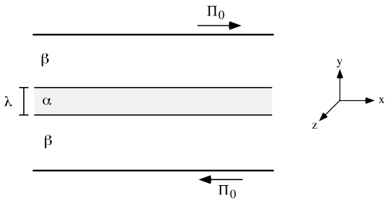
FIG. 1.: Geometry of a single lamellar domain of phase $\alpha$

II Model Equations

We consider a simple binary fluid with one scalar order parameter $\Phi$, the difference in concentration between the two components. We use the usual Ginzburg-Landau form for the coarse-grained free energy of a symmetrical mixture

$$F[\Phi]=\int dr\left(\frac{1}{2}K\left(\nabla\Phi\right)^{2}-\frac{1}{2}r_{o}\Phi^{2}+\frac{1}{4}g\Phi^{4}\right)\,,$$ (1)

where $r_{o}$ and $g$ are positive so that we are below the coexistence curve in the two-phase region. Minimizing the homogeneous part of $F$ leads to the values of the concentration in the two bulk phases at equilibrium:

$$\Phi=\pm\sqrt{\frac{r_{o}}{g}}\equiv\pm\phi_{e}\,.$$

The equation of motion for $\Phi$ is the Cahn-Hilliard equation with a convective coupling of $\Phi$ to the velocity field u:

$$\frac{\partial\Phi}{\partial t}=-{\bf u}\cdot\nabla\Phi+M\nabla^{2}\frac{\delta F}{\delta\Phi}\,.$$ (2)

Here $M$ is a concentration-independent mobility. Since we are interested in the late stages of phase separation, we neglect all thermal fluctuations. The equation for the velocity is the Navier-Stokes equation for an incompressible fluid, generalized to include the coupling of the order parameter to the velocity field [19]:

$$\rho\frac{\partial{\bf u}}{\partial t}+\rho({\bf u}\cdot\nabla){\bf u}=\eta\nabla^{2}{\bf u}+\nabla\Phi\frac{\delta F}{\delta\Phi}-\nabla P\,.$$ (3)

In this paper the viscosity $\eta$ will be taken to be independent of $\Phi$; hence there is a single viscosity for the fluid independent of the concentration pattern. The pressure $P$ is determined by the incompressibility condition

$$\nabla\cdot{\bf u}=0\,.$$ (4)

We will consider only low Reynold’s number flow so the convective term $({\bf u}\cdot\nabla){\bf u}$ in the Navier-Stokes equation can be ignored. We will also assume that the fluid is sufficiently viscous that the velocity responds instantaneously to slow changes in $\Phi$; we can then neglect the inertial term $\partial{\bf u}/\partial t$ and the resulting equations describe “creeping” or Stokes flow. The term coupling the concentration to the velocity field in (3) leads to a capillary force at interfaces, where gradients in $\Phi$ induce fluid flow. Eq. (2 - 4) are the same as those of “Model H” (without the thermal noise terms) used to study critical binary fluids [20]. These equations have been used extensively to study phase separation in binary fluids [3].

The first step in a stability analysis is to derive the steady-state solutions to the equations of motion. With the geometry of Fig. 1 in mind, we assume that $\Phi$ and u are functions of $y$ only and look for time-independent solutions. The Cahn-Hilliard equation (2) has steady state solutions satisfying

$$\frac{\delta F}{\delta\Phi}=-K\nabla^{2}\Phi-r_{o}\Phi+g\Phi^{3}=\mu={\rm constant}\,,$$ (5)

where $\mu$ is the exchange chemical potential. Near a single interface, we can take $\mu=0$ and the concentration has the usual “kink” solution

$$\Phi_{s}=\sqrt{\frac{r_{o}}{g}}\tanh\sqrt{\frac{r_{o}}{2K}}y=\phi_{e}\tanh y/\xi\,,$$ (6)

where the width of the interface between the two coexisting phases is the thermal correlation length $\xi=\sqrt{2K/r_{o}}$. For a system of many lamellar domains, Eq. (6) gives the concentration profile at each interface when the domain size is much larger than $\xi$. We note that there is a surface tension associated with the presence of an interface, which is just the excess free energy per unit area at the interface [21]:

$$\sigma=K\int_{-\infty}^{\infty}dy\left(\frac{d\Phi_{s}}{dy}\right)^{2}=\frac{2\sqrt{2}K^{1/2}r^{3/2}_{o}}{3g}=\frac{2\xi r_{o}^{2}}{3g}\,.$$ (7)

In the stationary state in shear flow there is no velocity in the $y$-direction. We impose a constant shear stress $\Pi_{0}$ so the stationary velocity satisfies

$${\bf u}_{s}={\dot{\gamma}}y{\hat{x}}$$ (8)

where

$$\dot{\gamma}\equiv\frac{\Pi_{0}}{\eta}$$

is the shear rate.

It is convenient to rewrite our equations in dimensionless form by scaling lengths by the correlation length, the concentration by its equilibrium magnitude in the bulk phases, and time by the natural diffusion time involving the mobility $M$ in the Cahn-Hilliard equation. The velocity is scaled by the correlation length over the diffusion time:

$${\bf\bar{r}} = {\bf r}\sqrt{\frac{r_{o}}{2K}}=\frac{{\bf r}}{\xi}\,,$$

$$\bar{t} = t\frac{Mr_{o}^{2}}{K}=t\frac{2Mr_{o}}{\xi^{2}},$$

$$\bar{\Phi} = \frac{\Phi}{\Phi_{e}}\,,$$

$${\bf\bar{u}} = {\bf u}\frac{K}{Mr_{o}^{2}\xi}={\bf u}\frac{\xi}{2Mr_{o}}\,,$$

$$\bar{P} = P\frac{\xi^{2}}{2K\phi_{e}^{2}}\,.$$

Note that the new dimensionless correlation length is $\bar{\xi}=1$. In dimensionless form the equations of motion are now

$$\frac{\partial\bar{\Phi}}{\partial\bar{t}} = -{\bf\bar{u}}\cdot\bar{\nabla}\bar{\Phi}+\frac{1}{2}\bar{\nabla}^{2}\left(-\frac{1}{2}\bar{\nabla}^{2}\bar{\Phi}-\bar{\Phi}+\bar{\Phi}^{3}\right)\,,$$ (9)

$$0 = \bar{\nabla}^{2}{\bf\bar{u}}+\frac{1}{\bar{\eta}}\bar{\nabla}\bar{\Phi}\left(-\frac{1}{2}\bar{\nabla}^{2}\bar{\Phi}-\bar{\Phi}+\bar{\Phi}^{3}\right)-\frac{1}{\bar{\eta}}\bar{\nabla}\bar{P}\,,$$ (10)

$$0 = \bar{\nabla}\cdot{\bf\bar{u}}\,.$$ (11)

We see that the system is characterized by the dimensionless parameter, $\bar{\eta}$:

$$\bar{\eta}=\frac{Mg\eta}{K}=\frac{4Mr_{o}\eta}{3\sigma\xi}\,.$$ (12)

In dimensionless form, the concentration and velocity profiles derived above for a single interface parallel to the flow are

$$\bar{\Phi}_{s}(\bar{y})=\tanh\bar{y}\,,$$ (13)

$$\bar{{\bf u}}_{s}(\bar{y})=\bar{\dot{\gamma}}\bar{y}\,{\bf\hat{x}}\,.$$ (14)

The dimensionless shear rate $\bar{\dot{\gamma}}=\dot{\gamma}t_{{\rm diff}}$ is simply the product of the shear rate and the diffusion time $t_{\rm{diff}}=\xi^{2}/Mr_{o}$, and thus represents a second dimensionless parameter that characterizes the strength of the shear flow.

III Stability Analysis

In this section we will develop an overall strategy to examine the stability of any number of lamellar domains. We perform a linear stability analysis about the stationary states derived above. We begin by considering small perturbations about the stationary solutions (we will drop the bars over the dimensionless variables in the rest of the discussion, except where noted):

$$\phi = \Phi-\phi_{s}\,,$$ (15)

$${\bf v} = {\bf u-u}_{s}\,.$$ (16)

To linear order in the perturbations $\phi$ and v the equations of motion become

$$\frac{\partial\phi}{\partial t}=-v_{y}\frac{\partial\phi_{s}}{\partial y}-u_{s}\frac{\partial\phi}{\partial x}+\frac{1}{2}\nabla^{2}\left(-\frac{1}{2}\nabla^{2}+W_{s}(y)\right)\phi\,,$$ (17)

$$0=\nabla^{2}{\bf v}+\frac{1}{\bar{\eta}}\frac{\partial\phi_{s}}{\partial y}\left(-\frac{1}{2}\nabla^{2}+W_{s}(y)\right)\phi{\bf\hat{y}}-\nabla P\,,$$ (18)

$$0=\nabla\cdot{\bf v}\,.$$ (19)

Here $W_{s}$ is a function of the stationary concentration profile:

$$W_{s}(y)=\left.\frac{\partial^{2}f}{\partial\phi^{2}}\right|_{{\displaystyle\phi_{s}(y)}}=-1+3\phi_{s}^{2}(y)\,.$$ (20)

For a single interface at $y=0$, $W_{s}(y)=2-3{\rm sech}^{2}y$ so that the nonconstant part of $W_{s}$ is isolated near the interface.

In this work we are interested in perturbations along the flow direction that are perpendicular to the planar interfaces. Any such perturbation can be written as a sum over Fourier components along the x-direction, so we take our perturbations to have the plane-wave forms

$$\phi=\phi(y){\rm e}^{ikx-\omega t}\,,\quad{\bf v}={\bf v}(y){\rm e}^{ikx-\omega t}\,.$$ (21)

We will consider long wavelength fluctuations for which $k\xi\ll 1$. Note that in the following, we take $k$ to be positive, so that $k$ represents the magnitude of the wavevector. First we consider the hydrodynamic equations. If we substitute the expression for ${\bf v}$ given in (21) into the equations of motion for ${\bf v}$, Eq. (18) and Eq. (19), we find we can solve them exactly in terms of a Green’s function. First we introduce the stream function $\Psi$, defined by

$$v_{x}=\frac{\partial\Psi}{\partial y},\quad v_{y}=-\frac{\partial\Psi}{\partial x}\,.$$ (22)

The incompressibility condition (19) is then automatically satisfied by $\Psi$. The two components of the Navier-Stokes equation (18) can be used to eliminate the pressure $P$, leaving a fourth-order ordinary differential equation for $\Psi=\psi(y)\exp(ikx-\omega t)$:

$$\psi^{(iv)}-2k^{2}\psi^{\prime\prime}+k^{4}\psi=\frac{ik}{\bar{\eta}}\phi_{s}^{\prime}\left(\frac{1}{2}k^{2}\phi-\frac{1}{2}\phi^{\prime\prime}+W_{s}(y)\phi\right)\,.$$ (23)

Here primes indicate differentiation with respect to $y$. The boundary conditions are that $\psi$ and its derivative vanish at infinity. This equation can be formally solved using a Green’s function, to obtain the $y$-component of ${\bf v}$ that is needed in the concentration equation (17):

$$v_{y}(y) = -ik\psi(y)$$ (24)

$$= \frac{1}{4\bar{\eta}k}\int_{-\infty}^{\infty}dy^{\prime}\left(1+k|y-y^{\prime}|\right){\rm e}^{\displaystyle{-k|y-y^{\prime}|}}\phi_{s}^{\prime}(y^{\prime})$$ (26)

$$\times\left(\frac{1}{2}k^{2}\phi(y^{\prime})-\frac{1}{2}\phi^{\prime\prime}(y^{\prime})+W_{s}(y^{\prime})\phi(y^{\prime})\right)\,.$$

This gives $v_{y}$ in terms of an integral over $\phi$.

Next substituting (21) into the concentration equation (17) results in an eigenvalue equation for $\omega(k)$:

$$\omega(k)\phi = v_{y}\frac{d\phi_{s}}{dy}+ik\dot{\gamma}y\phi$$ (28)

$$-\frac{1}{2}\left(\frac{d^{2}}{dy^{2}}-k^{2}\right)\left(-\frac{1}{2}\frac{d^{2}}{dy^{2}}+\frac{1}{2}k^{2}+W_{s}(y)\right)\phi\,,$$

where we have used $u_{s}=\dot{\gamma}y$. A real, positive value of $\omega(k)$ indicates stability (damping) of the perturbation. Note that this is essentially an integro-differential equation in which $v_{y}$ acts as an integral operator on $\phi$.

We cannot solve Eq. (28) exactly so an approximate method is needed. To develop our calculational approach we first consider Eq. (28) without the flow terms:

$$\omega\phi=-\frac{1}{2}\left(\frac{d^{2}}{dy^{2}}-k^{2}\right)\left(-\frac{1}{2}\frac{d^{2}}{dy^{2}}+\frac{1}{2}k^{2}+W_{s}(y)\right)\phi\,.$$ (29)

This equation is applicable to the perturbations of domains in a binary solid and was used by Langer [22] to describe coarsening mechanisms in binary alloys. Note that (29) has the form

$$\omega\phi={\mit\Gamma}F\phi\,,$$ (30)

where we have defined the operators

$${\mit\Gamma}=-\frac{1}{2}\left(\frac{d^{2}}{dy^{2}}-k^{2}\right)$$ (32)

$$F=-\frac{1}{2}\frac{d^{2}}{dy^{2}}+\frac{1}{2}k^{2}+W_{s}(y)\,.$$ (33)

If $\phi_{n}$ is the set of eigenfunctions of (30) and we define a set of “conjugate” functions by

$${\mit\Gamma}\tilde{\phi_{n}}=\phi_{n}\,,$$ (34)

then one can show that ${\mit\Gamma}$ and $F$ are Hermitian operators (although their product is not), as long as the $\phi_{n}$ and $\tilde{\phi_{n}}$ obey periodic boundary conditions or vanish at infinity. We note that the eigenvalues $\omega_{n}$ are real and the eigenfunctions and their conjugates are orthogonal:

$$(\tilde{\phi}_{m},\phi_{n})\equiv\int_{-\infty}^{\infty}\tilde{\phi}_{m}^{*}(y)\phi_{n}(y)dy=0\quad\rm{for}\quad n\neq m\,.$$

Then for any pair of trial functions $\phi_{0}$ and $\tilde{\phi}_{0}$ obeying the same boundary conditions, we can find an upper bound on the lowest eigenvalue $\omega$ from a variational relation [22, 23]

$$\omega_{min}\leq\frac{(\phi_{0},F\phi_{0})}{(\tilde{\phi}_{0},\phi_{0})}\,.$$ (35)

Here the parentheses again indicate inner products.

To apply Eq. (35) we need a good trial function $\phi_{0}$. It is easy to determine an exact solution of (29) in the particular case when we have a single flat interface present and when $\phi$ is a function of $y$ only ($k=0$). We note that the system is translationally invariant, so that any solution that corresponds to a translation of the interface by some amount $dy$ is also a solution. Thus if $y\rightarrow y+dy$ we can write

$$\phi_{s}(y+dy)=\phi_{s}+\frac{d\phi_{s}}{dy}dy+\cdots$$

so it must be that

$$\phi_{0}=\frac{d\phi_{s}}{dy}=\rm{sech}^{2}\mit{y}$$ (36)

is also a solution. It is easy to verify that this is the case, with corresponding eigenvalue $\omega=0$. This is the lowest lying eigenvalue of Eq. (29) for a system with a single planar interface and $k=0$ [23]. We can use the variational principle (35) to calculate the stability eigenvalues near this $\omega=0$ translational mode for more general situations by assuming a trial function formed by appropriate linear combinations of the single interface solution [24]. To use Eq. (35) we also need to determine the conjugate function $\tilde{\phi_{0}}$. By definition the conjugate function satisfies

$${\mit\Gamma}\tilde{\phi_{0}}=-\frac{1}{2}\left(\frac{d^{2}}{dy^{2}}-k^{2}\right)\tilde{\phi}_{0}(y)=\phi_{0}(y)\,.$$ (37)

We can easily solve for $\tilde{\phi}_{0}$ by using a Green’s function, with boundary conditions that $\tilde{\phi}_{0}$ and $\tilde{\phi}^{\prime}_{0}$ vanish at infinity. We find

$$\tilde{\phi}_{0}(y)=\int_{-\infty}^{\infty}dy^{\prime}\frac{1}{k}{\rm e}^{\displaystyle{-k\left|y-y^{\scriptstyle\prime}\right|}}\phi_{0}(y^{\prime})\,.$$ (38)

The conjugate function is thus obtained by substituting the desired trial function $\phi_{0}$ into Eq. (38).

To summarize the results of this section, we have linearized the equations of motion, expressed them parametrically in terms of the wavenumber $k$, and solved the hydrodynamic equations for $v_{y}$ as an integral over $\phi$. The eigenvalue equation (28) can be solved approximately in the absence of the two flow terms (i.e. Eq. (29)) by evaluating Eq. (35) using an appropriate trial function. The methods used to include the flow terms will be explained in the following sections.

IV Dispersion Relation for a Single Interface

As an example of the variational technique, consider the dispersion relation of a single flat interface separating semi-infinite domains of the two phases. We initially neglect hydrodynamic effects and focus on solving Eq. (29) for $\omega(k)$. For a single interface located at $y=0$ our trial solution is exactly $\phi_{0}=\phi_{s}^{\prime}=\rm{sech}^{2}\mit{y}$. There is only one term in $F\phi_{0}$, since $\phi_{0}$ is a solution to (29) for $k=0$:

$$F\phi_{0} = \left(-\frac{1}{2}\frac{d^{2}}{dy^{2}}+\frac{1}{2}k^{2}+2-3{\rm sech}^{2}y\right)\left({\rm sech}^{2}y\right)$$

$$= \frac{1}{2}k^{2}{\rm sech}^{2}y\,.$$

Using (38) for the conjugate function $\tilde{\phi_{0}}$, we find

$$\tilde{\phi_{0}}(y) = \int_{-\infty}^{\infty}dy^{\prime}\frac{1}{k}\exp(-k|y-y^{\prime}|){\rm sech}^{2}y^{\prime}$$

$$= \int_{-\infty}^{\infty}dy^{\prime}\left(\frac{1}{k}-|y-y^{\prime}|+\cdots\right){\rm sech}^{2}y^{\prime}$$

$$= \frac{2}{k}-2\ln\cosh y+O(k)\,,$$

where we have expanded the exponential for small $k$ (long wavelengths). This expansion is not uniform in $y$, but is justified since the integrand is only nonzero for small $y^{\prime}$ and because we will only need $\tilde{\phi_{0}}$ for small values of $y$ in the subsequent analysis. The normalization integral is simply

$$(\tilde{\phi}_{0},\phi_{0}) = \int_{-\infty}^{\infty}dy\,\left(\frac{2}{k}-2\ln\cosh y+O(k)\right){\rm sech}^{2}y$$

$$= \frac{4}{k}-2(2-2\ln 2)+O(k)\,.$$

Next we apply the variational theorem (35) to obtain

$$\omega \leq \frac{(\phi_{0},F\phi_{0})}{(\tilde{\phi}_{0},\phi_{0})}=\frac{2k^{2}/3}{4/k-2(2-2\ln 2)+O(k)}$$ (39)

$$\cong \frac{1}{6}k^{3}+O(k^{4})\,,$$ (40)

where we have retained only the lowest order term in $k$. If we rewrite this relation in dimensional units, we find

$$\omega\cong\frac{1}{3}Dk^{3}\xi+O(k^{4})$$ (41)

where $D=Mr_{o}$ is a diffusion constant. This result has been obtained previously by Jasnow and Zia [23] and by Shinozaki and Oono [25]. It also agrees to lowest order in $k$ with the perturbative calculation by Bettinson and Rowlands [26]. The eigenvalue is positive so the single interface is stable, at least to long wavelength perturbations.

The physics here is straightforward. We know that outside a curved interface there is a slight excess concentration, which is given by the Gibbs-Thomson relation [21]

$$\delta\phi=\frac{\sigma\chi}{R\Delta\phi}\,,$$ (42)

where $\sigma$ is the surface tension, $\chi$ is the susceptibility, $R$ is the radius of curvature of the interface, and $\Delta\phi=2\phi_{e}$ is the miscibility gap. In our case the curvature of the interface is $1/R=Ak^{2}$ where A is the amplitude of the small perturbation. The susceptibility $\chi$ is $\chi^{-1}=\partial\mu/\partial\phi=r_{o}$ in the bulk phase. The excess concentration due to the curvature is therefore

$$\delta\phi\sim\frac{Ak^{2}\sigma}{\phi_{e}r_{o}}\sim Ak^{2}\xi\phi_{e}\,,$$

where we have used (7) to eliminate $\sigma$. This excess concentration will occur outside regions of positive curvature, and there will be a corresponding lack of concentration in regions of negative curvature, creating a concentration gradient along the x-axis. The flux across the interface caused by this gradient is roughly $v\Delta\phi$ where $v$ is the velocity of the interface. That velocity, in turn, is just the rate of change of the amplitude $A$ of the perturbation, so

$$v\Delta\phi=\phi_{e}\frac{dA}{dt}=\phi_{e}\omega A\sim D\nabla\phi\,.$$

The concentration gradient is $\nabla\phi\sim k\delta\phi$; putting everything together, we find

$$\phi_{e}\omega A\sim DAk^{3}\xi\phi_{e}$$

so that $\omega\sim Dk^{3}\xi$ as advertised.

We can include the lowest order hydrodynamic effects on the dispersion relation by performing a perturbative calculation to first order in $k$. We write the full eigenvalue equation (28) in the form

$${\mit\Gamma}F\phi+V\phi=\omega\phi\,,$$ (43)

where the “unperturbed” problem is simply Eq. (29):

$${\mit\Gamma}F\phi_{0} = -\frac{1}{2}\left(\frac{d^{2}}{dy^{2}}-k^{2}\right)\left(-\frac{1}{2}\frac{d^{2}}{dy^{2}}+\frac{1}{2}k^{2}+W_{s}(y)\right)\phi_{0}$$

$$= \omega_{0}\phi_{0}\,,$$

with $\omega_{0}\cong k^{3}/6$ and $\phi_{0}\cong{\rm sech}^{2}y$ from the variational result (note these solutions are exact for $k=0$). The perturbation $V$ contains the flow terms

$$V=v_{y}\frac{d\phi_{s}}{dy}+ik\dot{\gamma}y\phi\,.$$

We expect $v_{y}$ to be proportional to a power of $k$ (since for $k=0$ there should be no induced velocity in the $y$-direction), so $V$ itself is proportional to a power of $k$ and is therefore small for long wavelengths. Expanding $\omega$ and $\phi$ in powers of $k$, and multiplying Eq. (43) on the left by the corresponding left eigenvector $\tilde{\phi}$, one can show in the usual way that the lowest order correction to $\omega$ in perturbation theory is

$$\omega_{1}=\frac{\left(\tilde{\phi_{0}},V\phi_{0}\right)}{\left(\tilde{\phi_{0}},\phi_{0}\right)}\,.$$ (44)

We solve for the velocity field by substituting $\phi_{0}$ into (26):

$$v_{y} = \frac{1}{4\bar{\eta}k}\int_{-\infty}^{\infty}dy^{\prime}\left(1+k|y-y^{\prime}|\right){\rm e}^{\displaystyle{-k|y-y^{\prime}|}}{\rm sech}^{2}y^{\prime}$$ (46)

$$\times\left(\frac{1}{2}k^{2}{\rm sech}^{2}y^{\prime}\right)$$

$$= \frac{k}{8\bar{\eta}}\int_{-\infty}^{\infty}dy^{\prime}\left({\rm sech}^{4}y^{\prime}+O(k^{2})\right)$$ (47)

$$= \frac{k}{6\bar{\eta}}+O(k^{2})\,,$$ (48)

where we have again expanded the exponential for small $k$. We find that to lowest order $v_{y}$ is linear in $k$, so that overall $V\propto k$. Since our first order perturbative result will only be good to $O(k)$, we only need the exact part of the result to the unperturbed problem (recall the variational result is $O(k^{3})$), for which $\omega_{0}=0$. In the reference frame in which $u_{s}(y)=\dot{\gamma}y$, the integral over the convective term $ik\dot{\gamma}y\phi$ in (44) vanishes, so that we obtain a single term in the first order correction to $\omega$ from the $v_{y}$ term:

$$\omega = \omega_{0}+\frac{\left(\tilde{\phi_{0}},v_{y}\phi_{s}^{\prime}\right)}{\left(\tilde{\phi_{0}},\phi_{0}\right)}$$ (49)

$$= 0+\frac{\left(\tilde{\phi_{0}},\left(k/6\bar{\eta}+O(k^{2})\right)\phi_{0}\right)}{\left(\tilde{\phi_{0}},\phi_{0}\right)}$$ (50)

$$= \frac{k}{6\bar{\eta}}+O(k^{2})\,,$$ (51)

since $\phi_{s}^{\prime}={\rm sech}^{2}y=\phi_{0}$ for a single interface. If we restore the units in this result we obtain

$$\omega=\frac{\sigma k}{4\eta}+O(k^{2})$$ (52)

where $\sigma$ is the surface tension. This is a well-known result for the damping of long wavelength capillary waves on a planar interface between two liquids, in the limit that the viscosity is sufficiently large that inertial effects can be neglected [27].

V Calculational Method for a Lamellar Domain

We now turn to the stability of a lamellar domain of one phase immersed in the other phase, so that we have two interfaces in the system as in Fig. 1. When the spacing $\lambda$ between the two interfaces is at least a few correlation lengths (note that we continue to work with scaled variables), $\lambda\gg 1$, the stationary concentration profile is

$$\phi_{s}=\left\{\begin{array}[]{ll}\tanh(y+\lambda/2)&-\infty<y<0\\ -\tanh(y-\lambda/2)&0<y<+\infty\end{array}\right.$$ (53)

where we have arbitrarily taken the $\alpha$ phase with equilibrium concentration $\phi_{\alpha}=+1$ to be in the middle, with layer thickness $\lambda$. In this expression we have set the exchange chemical potential $\mu$ to zero. More accurately, we can calculate $\mu$ as follows. The stationary solution that satisfies Eq. (5) is

$$\phi_{s}=\tanh(y+\lambda/2)-\tanh(y-\lambda/2)+\mu\,,$$

where the regions indicated in (53) are implied. The chemical potential serves as a Lagrange multiplier to keep the concentration conserved, so we can find $\mu$ by integrating the concentration field over the size of the system and setting it equal to the average concentration $\phi_{av}$:

$$\frac{1}{2L}\int_{-L}^{L}\phi_{s}(y)dy=\phi_{av}\,.$$

We want the volume fraction $x_{\beta}$ of the background phase with concentration $\phi_{\beta}=-1$ to be $x_{\beta}=(2L-\lambda)/2L$. Using the lever rule

$$x_{\beta}=\frac{\phi_{\alpha}-\phi_{av}}{\phi_{\alpha}-\phi_{\beta}}$$

and the equilibrium concentrations $\phi_{\alpha}=1$, $\phi_{\beta}=-1$ we find that

$$\phi_{av}=-1+\frac{\lambda}{L}\,.$$

Doing the integral over the stationary concentration and keeping only the first order corrections in $\exp(-\lambda)$ for $\lambda\gg 1$, we find that

$$\mu\cong-\frac{1}{L}{\rm e}^{-\lambda}\,,$$ (54)

so that $\mu\rightarrow 0$ as the system size $L\rightarrow\infty$. The dependence of $\mu$ on $\lambda$ will be important to our understanding of the physics in Section VI A below.

Next we want to solve the full eigenvalue equation (28) for the lamellar domain. Any perturbation of the domain can be written in terms of two linearly independent perturbation modes: either the two interfaces can fluctuate in phase with each other to form a “zig-zag” mode, or they can fluctuate out of phase in a “varicose” or “peristaltic” mode. These modes are pictured in Fig. 2 and Fig. 3. Since we are interested in calculating the eigenvalues near the marginally stable mode with $\omega=0$ at $k=0$, we take the perturbed concentration field for the ziz-zag and varicose modes to be, respectively,

$$\phi_{z} = \frac{1}{2}{\rm sech}^{2}(y+\lambda/2)-\frac{1}{2}{\rm sech}^{2}(y-\lambda/2)\,,$$ (55)

$$\phi_{v} = \frac{1}{2}{\rm sech}^{2}(y+\lambda/2)+\frac{1}{2}{\rm sech}^{2}(y-\lambda/2)\,.$$ (56)

The variational theorem (35) gives the eigenvalues for these two modes in the absence of any hydrodynamic effects. However, we are interested in the effect of the shear flow and of the fluid flow induced by gradients in the concentration. We cannot use the perturbation theory approach used in Section IV because the varicose mode is not a solution to any “unperturbed” operator in Eq. (28) (note that the zig-zag mode is the translation mode, $\phi_{z}=\phi_{s}^{\prime}$, and is an exact solution to (29) at $k=0$). Instead, we adopt a “tight-binding” approximation that will allow us to solve the full problem.

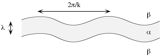
FIG. 2.: Zig-zag mode

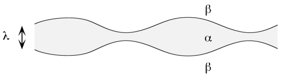
FIG. 3.: Varicose mode

To implement this approach, we consider the two perturbation modes above to be two basis states, and rewrite the eigenvalue equation (28) as a two-by-two matrix equation in this basis. We use $\phi$ as the right-hand basis state and the conjugate function $\tilde{\phi}$ as the left-hand state. We insert our two trial functions (55) and (56) for $\phi$ into the eigenvalue equation, multiply on the left by the corresponding $\tilde{\phi}$, and integrate over all $y$. In vector notation, we have

$$\phi_{0} = \left(\begin{array}[]{c}a({\rm sech}^{2}(y+\lambda/2)-{\rm sech}^{2}(y-\lambda/2))/2\\ b({\rm sech}^{2}(y+\lambda/2)+{\rm sech}^{2}(y-\lambda/2))/2\end{array}\right)$$ (59)

$$= \left(\begin{array}[]{c}a\phi_{z}\\ b\phi_{v}\end{array}\right)$$ (62)

as our trial function, where $a$ and $b$ are the amplitudes of the two modes. Substituting into Eq. (28) gives the matrix equation

$$\left(\begin{array}[]{cc}(\tilde{\phi_{z}},\phi_{z})\omega&0\\ 0&(\tilde{\phi_{v}},\phi_{v})\omega\end{array}\right)\left(\begin{array}[]{c}a\\ b\end{array}\right)=$$ (72)

$$\left(\begin{array}[]{cc}(\tilde{\phi}_{z},v_{y}^{z}\phi_{s}^{\prime})+(\tilde{\phi}_{z},ik\dot{\gamma}y\phi_{z})+(\phi_{z},F\phi_{z})&(\tilde{\phi}_{z},v_{y}^{v}\phi_{s}^{\prime})+(\tilde{\phi}_{z},ik\dot{\gamma}y\phi_{v})\\ (\tilde{\phi}_{v},v_{y}^{z}\phi_{s}^{\prime})+(\tilde{\phi}_{v},ik\dot{\gamma}y\phi_{z})&(\tilde{\phi}_{v},v_{y}^{v}\phi_{s}^{\prime})+(\tilde{\phi}_{v},ik\dot{\gamma}y\phi_{v})+(\phi_{v},F\phi_{v})\end{array}\right)\left(\begin{array}[]{c}a\\ b\end{array}\right)\,.$$

Here we have used the definition ${\mit\Gamma}\tilde{\phi}=\phi$. The superscript on $v_{y}$ indicates with which perturbation mode the velocity field corresponds, so that $v_{y}^{z}$ is the velocity induced by the zig-zag mode and $v_{y}^{v}$ the velocity induced by the varicose mode. On the left-hand side of (72) we use the orthogonality properties

$$(\tilde{\phi}_{z},\phi_{v})=(\tilde{\phi}_{v},\phi_{z})=0\,.$$

These also apply to the diffusive terms on the right-hand side; this procedure thus ensures that in the absence of any flow effects we obtain the same eigenvalues $\omega$ as we would from the variational theorem (35). We can now solve (72) for the stability eigenvalues. Note that all calculations presented below are carried out to the lowest possible order in $k$.

VI Lamellar Domain Results

A Without Shear Flow

We consider first the solution of (72) in the absence of the external shear flow ($\dot{\gamma}=0$). The only possible off-diagonal terms are the ones involving $v_{y}$. We begin by calculating the necessary integrals that form the matrix elements.

Using Eq.  (38) and expanding for small $k$ as in Section IV, we find the conjugate function for the zig-zag mode is

$$\tilde{\phi_{z}}(y)=-\ln\cosh(y+\lambda/2)+\ln\cosh(y-\lambda/2)+k\lambda y+O(k^{2})\,.$$

The normalization integral is then

$$(\tilde{\phi}_{z},\phi_{z}) = \int_{-\infty}^{\infty}dy\left\{\left(-\ln\cosh(y+\lambda/2)\right.\right.$$ (75)

$$\;\left.\left.+\ln\cosh(y-\lambda/2)+k\lambda y+O(k^{2})\right)\right.$$

$$\left.\times\left({\rm sech}^{2}(y+\lambda/2)+{\rm sech}^{2}(y-\lambda/2)\right)\right/2\}$$

$$= 2\lambda-2-k\lambda^{2}+O(k^{2})\,.$$ (76)

Note that the second term on the right hand side of the above is negligible for sufficiently large $\lambda$, but not when $\lambda$ is of the order of a few correlation lengths. Since it is reasonable to consider the case of $\lambda$ being a few times $\xi$ (recall $\xi=1$), we consider $\exp(-\lambda)$ to be a small parameter in the calculation, but not $1/\lambda$, so that we retain terms like the additive $2$ in (76). Next, substituting $\phi_{z}$ into Eq. (26) for the velocity field, we find by expanding for small $k$ as before,

$$v_{y}^{z}(y)=\frac{k}{6\bar{\eta}}-\frac{k^{3}}{48\bar{\eta}}\left(4y^{2}+\lambda^{2}+\frac{\pi^{2}}{3}-2\right)+O(k^{4})\,.$$ (77)

Finally, since $\phi_{z}=\phi_{s}^{\prime}$, there is only one term in $F\phi_{z}$:

$$F\phi_{z}=\frac{1}{4}k^{2}({\rm sech}^{2}(y+\lambda/2)-{\rm sech}^{2}(y-\lambda/2))\,.$$ (78)

Now we turn to the varicose mode. The conjugate function for this mode, expanded for small $k$, is

$$\tilde{\phi}_{v}(y) = \frac{2}{k}-\ln\cosh(y+\lambda/2)-\ln\cosh(y-\lambda/2)$$

$$+k\left(y^{2}+\frac{\lambda^{2}}{4}+\frac{\pi^{2}}{12}\right)+O(k^{2})\,.$$

This leads to a normalization integral of

$$(\tilde{\phi}_{v},\phi_{v})=\frac{4}{k}-2\lambda-2+4\ln 2+k\left(\lambda^{2}+\frac{\pi^{2}}{3}\right)+O(k^{2})\,.$$

We note that the normalization goes to infinity as $k\rightarrow 0$. This is the mathematical manifestation of the fact that the varicose mode is not allowed at $k=0$ because it does not conserve mass. For any nonzero $k$ however there is no problem. The velocity field for the varicose mode is given by

$$v_{y}^{v}(y)=\frac{4k}{\bar{\eta}}\left(2\lambda-3\right){\rm e}^{-2\lambda}y-\frac{k^{3}\lambda}{12\bar{\eta}}y+O(k^{2}{\rm e}^{-2\lambda},k^{4})\,.$$ (79)

In this expression we have not included terms of $O(k^{2}{\rm e}^{-2\lambda})$. These terms will be negligible compared to terms of $O(k^{3})$ for $k>{\rm e}^{-2\lambda}$ (at such small $k$, of course, the linear term in $k$ will dominate over any $k^{2}$ terms). We will see below that this condition is met for the $k$ values of most interest. Finally, for the varicose mode

$$F\phi_{v} = \frac{1}{4}k^{2}({\rm sech}^{2}(y+\lambda/2)+{\rm sech}^{2}(y-\lambda/2))$$ (81)

$$-3{\rm sech}^{2}(y+\lambda/2){\rm sech}^{2}(y-\lambda/2)\,,$$

so that $F\phi_{v}$ includes an overlap term between the two interfaces.

It is fairly simple to show by straightforward integration that the off-diagonal terms in (72) vanish (for $\dot{\gamma}=0$):

$$(\tilde{\phi}_{z},v_{y}^{v}\phi_{s}^{\prime})=(\tilde{\phi}_{v},v_{y}^{z}\phi_{s}^{\prime})=0\,.$$

This reduces the matrix equation to

$$\left(\begin{array}[]{cc}(\tilde{\phi_{z}},\phi_{z})\omega&0\\ 0&(\tilde{\phi_{v}},\phi_{v})\omega\end{array}\right)\left(\begin{array}[]{c}a\\ b\end{array}\right)=\left(\begin{array}[]{cc}(\tilde{\phi_{z}},v_{y}^{z}\phi_{s}^{\prime})+(\phi_{z},F\phi_{z})&0\\ 0&(\tilde{\phi_{v}},v_{y}^{v}\phi_{s}^{\prime})+(\phi_{v},F\phi_{v})\end{array}\right)\left(\begin{array}[]{c}a\\ b\end{array}\right)$$ (82)

so that we can solve for each eigenvalue separately:

$$\omega=\frac{(\tilde{\phi},v_{y}\phi_{s}^{\prime})+(\phi,F\phi)}{(\tilde{\phi},\phi)}$$ (83)

for each mode. Using the expressions given above we perform the remaining integrals to obtain $\omega$ for each mode.

For the zig-zag mode we find

$$\omega_{z} \cong \frac{k}{3\bar{\eta}}+\frac{k^{2}}{6(\lambda-1)}\left(1+\frac{k\lambda^{2}}{2\lambda-2}\right)$$ (85)

$$-\frac{k^{3}}{12\bar{\eta}}\left(\lambda^{2}+\frac{\pi^{2}}{6}-1+f(\lambda)\right)+O(k^{4})\,,$$

where $f(\lambda)$ is the function

$$f(\lambda)=\frac{\delta_{2}(\lambda)-\lambda\delta_{1}(\lambda)-\delta_{0}}{\lambda-1}\,.$$

Here $\delta_{0}$ is the definite integral

$$\delta_{0}=\int_{-\infty}^{\infty}dy\,y^{2}{\rm sech}^{2}y\ln\cosh y=1.70681\,,$$

and the functions $\delta_{1}$ and $\delta_{2}$ are the overlap integrals

$$\delta_{1}(\lambda)=\int_{-\infty}^{\infty}dy\,y{\rm sech}^{2}y\ln\cosh(y-\lambda)\,,$$

$$\delta_{2}(\lambda)=\int_{-\infty}^{\infty}dy\,y^{2}{\rm sech}^{2}y\ln\cosh(y-\lambda)\,.$$

These are integrated numerically using Mathematica. We see from Eq. (85) that the zig-zag mode is stable for small $k$. The terms involving the dimensionless viscosity $\bar{\eta}$ are due to the flow field induced by the perturbations in the concentration $\phi$, and come from the $v_{y}$ term in (28). Depending on the value of $\bar{\eta}$, either the hydrodynamic terms or the diffusive terms will dominate. We find that the stability eigenvalue for the varicose mode is

$$\omega_{v} \cong -8k{\rm e}^{-2\lambda}-\frac{12k\lambda{\rm e}^{-2\lambda}}{\bar{\eta}}\left(\frac{2}{3}\lambda-1\right)+\frac{k^{3}}{12}$$ (87)

$$+\frac{k^{3}\lambda^{2}}{6\bar{\eta}}+O(k^{2}{\rm e}^{-2\lambda},k^{4})\,.$$

The varicose mode is thus unstable for sufficiently small wavelengths! The eigenvalues for the two modes are plotted as functions of $k$ in Fig. 4. Here we take $\lambda=6$, so that ${\rm e}^{-2\lambda}$ is small (as we assumed above) and $k>{\rm e}^{-2\lambda}$ for most of the range in the graph, as discussed above. We take the dimensionless viscosity to be $\bar{\eta}=.1$, which is a typical value for critical binary fluids. However the overall shape of the dispersion relations remains similar for other values of $\lambda$ and $\bar{\eta}$.

The instability of the varicose mode may seem unintuitive. We first note that it is unstable only for sufficiently small $k$, and is stabilized at larger wavenumbers by the $k^{3}$ curvature term, the same term that was obtained in Eq. (40) for a system with a single interface. Second, the instability is exponentially small in the separation between the interfaces, $\lambda$. This is thus a very weak instability. It is due to a coarsening effect (essentially Ostwald ripening) in which thin regions of the middle phase shrink in favor of fatter regions. Recall that the chemical potential $\mu\sim{\rm e}^{-\lambda}$. If $\lambda$ decreases in a region, $\mu$ increases, so the chemical potential is higher in the neck regions than in the bulges. This drives a flux from the necks towards the bulges (see Fig. 5). We can understand the lowest order diffusive effect as follows. First note that the lowest order diffusion term in Eq. (87), with units, is

$$\omega\sim-16D\frac{k}{\xi}{\rm e}^{-2\lambda/\xi}$$

As before, we can express the velocity of the interface $\omega A$ as

$$\omega A\phi_{e}\sim D\nabla\phi\sim Dk\delta\phi$$

since the concentration gradient is along the x-direction. The excess concentration added (subtracted) in the bulk regions of the necks (bulges) is essentially

$$\delta\phi\sim\frac{A\phi_{e}}{\xi}{\rm sech}^{2}y/\xi\sim\frac{A\phi_{e}}{\xi}{\rm e}^{-2\lambda/\xi}$$

so that

$$\omega\sim-D\frac{k}{\xi}{\rm e}^{-2\lambda/\xi}$$

This implies that a large sheet of one phase immersed in the other will break up into cylinders via this instability. Note that this is not the Rayleigh instability of a long fluid cylinder, in which the cylinder is unstable towards long wavelength, axisymmetric fluctuations. That is a hydrodynamic instability that occurs for a three-dimensional cylindrical interface because the curvature at the necks is higher than at the bulges. In this two-dimensional perturbation mode, the curvature at the necks and bulges is of the same magnitude (the extra dimension out of the plane of say Fig. 5 does not exist), and so there is no curvature-driven instability. The curvature effect is stabilizing, and it is the thermodynamic force driving phase separation that causes the instability.

FIG. 4.: Dispersion relation for $\dot{\gamma}=0$, with $\lambda=6$ and $\bar{\eta}=.1$

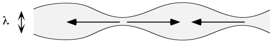
FIG. 5.: Diffusional instability of the varicose mode

B With Shear Flow

Next we consider what happens when we include the external shear flow. Physically, the shear flow tends to mix the two modes since the top interface travels in an opposite direction to the bottom interface. We might then expect that at some shear rate, the two perturbation modes lose their distinguishing features.

To calculate the eigenvalues we only need to calculate the matrix elements involving the shear. It is straightforward to show that the operator $ik\dot{\gamma}y$ is off-diagonal in the basis of our two perturbation modes, i.e.

$$(\tilde{\phi}_{z},ik\dot{\gamma}y\phi_{z})=(\tilde{\phi}_{v},ik\dot{\gamma}y\phi_{v})=0\,.$$

These two off-diagonal elements are found to be

$$(\tilde{\phi}_{z},ik\dot{\gamma}y\phi_{v}) = ik\dot{\gamma}(\lambda-\lambda^{2}+\delta_{1})+ik^{2}\dot{\gamma}\lambda\left(\frac{\lambda^{2}}{2}+\frac{\pi^{2}}{6}\right)$$ (89)

$$+O(k^{3})\,,$$

$$(\tilde{\phi}_{v},ik\dot{\gamma}y\phi_{z}) = -2i\dot{\gamma}\lambda+ik\dot{\gamma}(\lambda-2\lambda\ln 2-\delta_{1}+\lambda^{2})$$ (91)

$$-ik^{2}\dot{\gamma}\left(\frac{\lambda^{3}}{2}+\frac{\pi^{2}\lambda}{3}\right)+O(k^{3})\,.$$

The stability eigenvalues are now found by diagonalizing Eq. (72), which means solving the secular equation

$$\left|\begin{array}[]{cc}\omega_{z}-\omega&(\tilde{\phi}_{z},ik\dot{\gamma}y\phi_{v})/(\tilde{\phi}_{z},\phi_{z})\\ (\tilde{\phi}_{v},ik\dot{\gamma}y\phi_{z})/(\tilde{\phi}_{v},\phi_{v})&\omega_{v}-\omega\end{array}\right|=0\,.$$ (92)

Solving for $\omega$ gives

$$\omega_{\pm}(k)=\frac{1}{2}(\omega_{z}(k)+\omega_{v}(k))\pm\frac{1}{2}\sqrt{\left(\omega_{z}(k)-\omega_{v}(k)\right)^{2}-\dot{\gamma}^{2}s(k)}\,,$$ (93)

where $s(k)$ is given by

$$s(k)=\frac{k^{2}\lambda(\lambda^{2}-\lambda-\delta_{1})}{\lambda-1}+\frac{k^{3}}{2(\lambda-1)}\left[\left(\delta_{1}+\frac{\lambda^{3}}{\lambda-1}\right)(\lambda^{2}-\lambda-\delta_{1})-\lambda^{4}-\frac{\pi^{3}}{3}\lambda^{2}\right]+O(k^{4})\,.$$ (94)

Some examples of the two curves $Re(\omega_{\pm}(k))$ are shown in Fig. 6. The spacing between the two interfaces is $\lambda=6\xi$ and we have taken $\bar{\eta}=.1$. For $\dot{\gamma}=0$ it is clear that (93) reduces to our previous results, with $\omega_{+}=\omega_{z}$ and $\omega_{-}=\omega_{v}$. Fig. 6 shows $\omega_{-}$ for three different shear rates (it turns out that the curves for $\omega_{+}$ for these same shear rates are nearly indistinguishable, so they are plotted as one curve in Fig. 6). We see that at low shear rates the unstable mode still exists, but the window of wavenumbers over which $Re(\omega_{-})<0$ becomes smaller as $\dot{\gamma}$ increases. Above some critical shear rate $\dot{\gamma}_{c}$, the previously unstable mode becomes stable for all $k$. The shear flow thus completely stabilizes the varicose mode, by mixing it with the stable zig-zag mode.

FIG. 6.: Dispersion relations: $\omega_{+}$ for $\dot{\gamma}=.04$ (solid line); $100\omega_{-}$ for $\dot{\gamma}=.04$ (dashed), $\dot{\gamma}=\dot{\gamma}_{c}=.07225$ (dotted), and $\dot{\gamma}=.1$ (dash-dot)

We can easily solve for the critical shear rate $\dot{\gamma}_{c}$. First note that the first term in (93) is positive, because the negative terms in $\omega_{v}$ are exponentially small in $\lambda$. As $\dot{\gamma}$ is increased, the square root term in (93) becomes smaller. The effect is that the value of $k$ below which $\omega_{-}<0$ becomes smaller with increasing shear; the domain is only unstable to longer and longer wavelength perturbations as the shear rate is increased. For a given shear rate, $\omega_{-}>0$ for all $k>k_{c}$ where $k_{c}$ satisfies $\omega_{-}(k_{c})=0$:

$$\omega_{z}(k_{c})+\omega_{v}(k_{c})=\sqrt{\left(\omega_{z}(k_{c})-\omega_{v}(k_{c})\right)^{2}-\dot{\gamma}^{2}s(k_{c})}\,.$$ (95)

The unstable mode becomes stable for all wavenumbers $k$ when $k_{c}\rightarrow 0$. To find the critical shear rate, we first solve (95) for $\dot{\gamma}(k_{c})$:

$$\dot{\gamma}^{2}(k_{c})=\frac{-4\omega_{z}(k_{c})\omega_{v}(k_{c})}{s(k_{c})}\,.$$ (96)

Taking the limit $k_{c}\rightarrow 0$ in Eq. (96) gives the critical shear rate for complete stabilization:

$$\dot{\gamma}_{c}^{2}=\frac{4(\lambda-1){\rm e}^{-2\lambda}(8\bar{\eta}+4\lambda(2\lambda-3))}{3\bar{\eta}^{2}\lambda\left(\lambda^{2}-\lambda+\delta_{1}(\lambda)\right)}\,.$$ (97)

For the specific values $\lambda=6$ and $\bar{\eta}=.1$, one finds $\dot{\gamma}_{c}=.07225$ as indicated in Fig. 6.

The critical shear rate is graphed as a function of $\bar{\eta}$ and $\lambda$ in Fig. 7 and Fig. 8. We note the lamella is stable for all $\dot{\gamma}>\dot{\gamma}_{c}$. We see that $\dot{\gamma}_{c}$ is an algebraically decreasing function of $\bar{\eta}$ and an exponentially decreasing function of $\lambda$. Recall that $\bar{\eta}=4D\eta/3\sigma\xi$, so that (97) tells us that as the viscosity increases, or alternatively as the surface tension decreases, the easier it is for the shear flow to mix the two modes before the unstable perturbation has a chance to grow. We can also invert (97) to obtain the critical width $\lambda_{c}$ above which the lamella is stable for a given shear rate $\dot{\gamma}$. As we see from Fig. 8, given a shear rate $\dot{\gamma}$, at values of $\lambda$ lying below the curve the lamella is unstable to the varicose coarsening mode whereas for values of $\lambda$ above the curve the lamella is stable and will no longer coarsen. This simple system of a single lamellar domain thus exhibits the well-known experimental observation that the shear flow tends to halt the phase separation process.

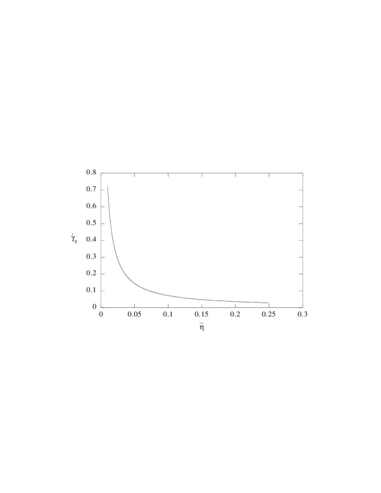
FIG. 7.: Critical shear rate $\dot{\gamma}_{c}(\bar{\eta})$ for $\lambda=6$

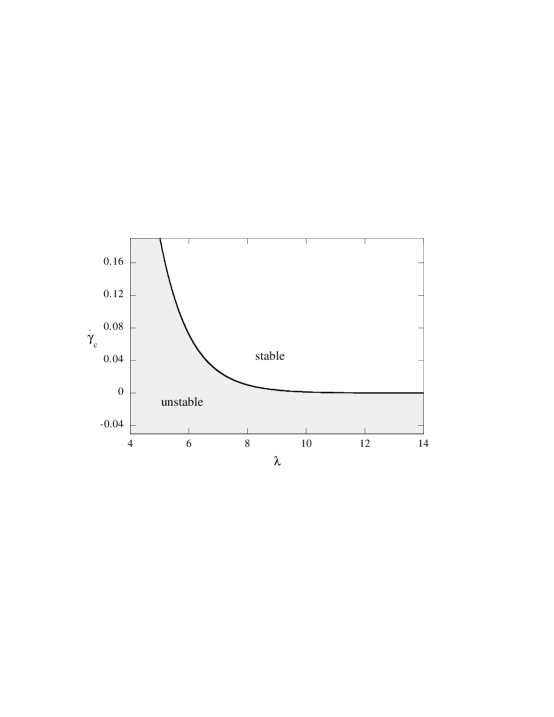
FIG. 8.: Critical shear rate $\dot{\gamma}_{c}(\lambda)$ for $\bar{\eta}=.1$

VII Discussion

We have seen that in the case of an isolated lamellar domain, shear flow has the effect of mixing the zig-zag and varicose modes so that they both become stable. Essentially, the flow eliminates the special phase relationship between the two interfaces necessary for the varicose mode to exist. The physics of this mode is that thin regions evaporate in favor of thick regions, but in the presence of shear thin and thick regions do not exist long enough for this diffusion to take place since the fluctuations are being carried downstream.

We would expect that a similar mechanism would apply to a large stack (along the $y$-direction) of lamellar domains. Although the stability eigenvalues have not been calculated for this case, the effects seen in the single lamellar domain should apply. Coarsening in the $y$ direction in a stack of lamellae is also dependent on thinner regions evaporating, their atoms diffusing across the intervening phase to a thicker region. From [22] we expect this coarsening instability to also have a rate that is exponentially small in $\lambda$. When one considers sinusoidal perturbations of the layers in a shear flow, once again the phase relations between interfaces will be constantly changing. As $\lambda$ increases, the atoms must diffuse farther across a layer for the pattern to coarsen, but they must be able to do so before they are swept downstream by the shear flow to a new $x$ position where the diffusion is no longer favored. We might anticipate then that in a general two-dimensional system with many lamellar domains, for any given shear rate $\dot{\gamma}$ there is an upper limit $\lambda_{c}$ to the layer spacing for which the coarsening instability is still present. The shear flow destroys the correlations between interfaces necessary for the coarsening instability to operate, leading to a dynamic steady state. The strength of the shear flow would determine the typical lamellar width $\lambda_{c}(\dot{\gamma})$ present in the system at steady state.

This behavior is qualitatively similar to that seen in the fully three dimensional “string” phase in shear flow. We do not expect quantitative agreement, however, because the stability analysis of the lamellar domain considered here is strongly dependent on the dimensionality. The instability of a long cylinder is much stronger than the weak exponential (2D) instability found here. For the case of a viscous cylinder of fluid immersed in another viscous liquid, the hydrodynamic instability corresponding to a varicose perturbation has a dispersion relation that behaves as [16]

$$\omega\sim-\frac{\sigma}{2\eta a}f(ka)$$

where $a$ is the radius of the cylinder. Thus, we might expect more dramatic effects in this case.

In summary, we have shown that a long extended domain in the two-phase state of a two-dimensional, phase-separating binary fluid can be stabilized by an applied shear flow. There is a critical shear rate below which the extended domain is unstable towards long wavelength fluctuations and above which we predict complete stabilization. This is in qualitative agreement with experiments on dynamic steady states in phase-separating fluids under shear flow, however the mechanisms operative here are different due to the reduced dimensionality. We intend to report results of a similar calculation for a long cylindrical domain under flow in the future.

REFERENCES

• [1] E.ย D. Siggia, Phys. Rev. A 20, 595 (1979).
• [2] A. Onuki, Europhys. Lett. 28, 175 (1994).
• [3] A.ย J. Bray, Advances in Physics 43, 357 (1994).
• [4] T. Imaeda, A. Onuki, and K. Kawasaki, Prog. Theor. Phys. 71, 16 (1984).
• [5] A. Onuki, Phys. Rev. A 34, 3528 (1986).
• [6] T. Ohta, H. Nozaki, and M. Doi, J. Chem. Phys. 93, 2664 (1990).
• [7] P. Padilla and S. Toxvaerd, J. Chem. Phys. 106, 2342 (1997).
• [8] T. Baumberger, F. Perrot, and D. Beysens, Physica A 174, 31 (1991).
• [9] C. Chan, F. Perrot, and D. Beysens, Phys. Rev. A 43, 1826 (1991).
• [10] J. Lรคuger, C. Laubner, and W. Gronski, Phys. Rev. Lett. 75, 3576 (1995).
• [11] T. Hashimoto, T. Takebe, and S. Suehiro, J. Chem. Phys. 88, 5874 (1988).
• [12] K. Min and W. Goldberg, Phys. Rev. Lett. 70, 469 (1993).
• [13] T. Hashimoto, K. Matsuzaka, E. Moses, and A. Onuki, Phys. Rev. Lett. 74, 126 (1995).
• [14] E.ย K. Hobbie, S. Kim, and C.ย C. Han, Phys. Rev. E 54, 5909 (1996).
• [15] Lord Rayleigh, Philos. Mag. 34, 145 (1892).
• [16] S. Tomotika, Proc. Roy. Soc. London A 150, 322 (1935).
• [17] K. Hamano etย al., Phys. Rev. E 51, 1254 (1995).
• [18] M.ย S. Miguel, M. Grant, and J.ย D. Gunton, Phys. Rev. A 31, 1001 (1985).
• [19] P. Chaikin and T. Lubensky, Principles of Condensed Matter Physics (Cambridge University Press, Cambridge, 1995), p.ย 476.
• [20] P.ย C. Hohenberg and B.ย I. Halperin, Rev. Mod. Phys. 49, 435 (1977).
• [21] J.ย S. Langer, in Solids Far from Equilibrium, Proc. 1989 Beg Rohu Summer School, edited by C. Godreche (Cambridge University Press, Cambridge, 1992).
• [22] J.ย S. Langer, Annals of Phys. 65, 53 (1971).
• [23] D. Jasnow and R.ย K.ย P. Zia, Phys. Rev. A 36, 2243 (1987).
• [24] For a more rigorous analysis of the structure of the stability eigenvalues, see [25] and A. Shinozaki, Phys. Rev. E 48, 1984 (1993).
• [25] A. Shinozaki and Y. Oono, Phys. Rev. E 47, 804 (1993).
• [26] D. Bettinson and G. Rowlands, Phys. Rev. E 54, 6102 (1996).
• [27] See e.g.ย C.ย A. Miller and P. Neogi, Interfacial Phenomena: Equilibrium and Dynamic Effects (Marcel Dekker, Inc., New York, 1985), p.ย 199; S. Chandrasekhar, Hydrodynamic and Hydromagnetic Stability (Dover Publications, Inc., New York, 1981), p.ย 443, the limit as $\nu\rightarrow 0$ of Eq. (115).