[

Aging in the linear harmonic oscillator

Abstract

The low temperature Monte Carlo dynamics of an ensemble of linear harmonic oscillators shows some entropic barriers related to the difficulty of finding the directions in configurational space which decrease the energy. This mechanism is enough to observe some typical non-equilibrium features of glassy systems like activated-type behavior and aging in the correlation function and in the response function. Due to the absence of interactions the model only displays a one-step relaxation process.

]

Slow relaxation processes are widespread in condensed matter physics. These include magnetic relaxation in spin glasses, transport processes in structural glasses, pinning effects in superconductors among others. A large class of these systems show what is commonly referred as aging, i.e. dependence of the response of the system on the time in which it is perturbed. Aging effects [1] are a signature that the system is far from thermal equilibrium and consequently the fluctuation-dissipation theorem is not valid [2]. It has been realized quite recently that aging is indeed a solution of the off-equilibrium dynamics in some exactly solvable models [3, 4]. Aging appears if relaxation to the equilibrium is slow due to the presence of energy barriers in a rugged free energy landscape as well as in systems with entropy barriers with a quite simple landscape [5, 6]. In this last case, as the system relaxes towards the equilibrium, the number of directions in phase space where the system can move decreases progressively. This means that the system needs more time to decorrelate or to forget the previous configuration. This effect is usually encoded in the two time correlation function where the $C(t,t^{\prime})$ depends on both time indices [7].

From previous considerations it is clear that aging can also be present in extremely simple relaxing systems without any interaction, the only condition being the progressive reduction of available phase space where the energy decreases. This was an essential ingredient in the Backgammon model recently proposed to explain glassy behavior in the absence of energy barriers [5]. Here we consider a simpler example and analyze the Brownian oscillator. The Brownian oscillator is usually studied in the Langevin approach. It is described in any textbook of stochastic theory [8]. It is possible to show that in this case there are no slow processes involved. In fact, the relaxation turns out to be exponential as expected for the dynamics of a particle in a single parabolic potential well. Here we consider the Monte Carlo approach and choose a dynamics based on the Metropolis algorithm [9]. This Monte Carlo approach was already studied in a disordered model with long-range interactions which turns out to be non trivial, at least in the zero temperature limit [10]. The simplest case of an harmonic oscillator is solvable and we analyze the dynamics here.

In [10] we checked that, after a suitable rescaling of time, the equilibrium Langevin and Monte Carlo dynamics are equivalent. Also, we showed how the Langevin dynamics can be derived from the Monte Carlo dynamics in the limit of small changes. Here, we will see that the same results are valid. We will obtain the dynamical equations for the energy, the correlation and the response function. We will also study the low temperature dynamics, showing the similarities and differences with more realistic models for glasses.

The harmonic oscillator has an energy,

$$E=\frac{1}{2}Kx^{2}$$ (1)

where $K$ is the Hooke constant and $x$ defines the position of the harmonic particle. Let us consider an ensemble of $N$ independent linear oscillators with total energy $E(\{x_{i}\})=(K/2)\sum_{i}x_{i}^{2}$. A change of $\{x_{i}\}$ is proposed $\{x_{i}\to x^{\prime}_{i}=x_{i}+r_{i}/\sqrt{N},\forall i\}$ where $\{r_{i}\}$ is randomly chosen for each oscillator from a Gaussian distribution of zero mean and finite variance equal to $\Delta^{2}$. The change is accepted with probability $1$ if the energy decreases, i.e. if $\delta E=E(\{x^{\prime}_{i}\})-E(\{x_{i}\})$ is negative. Otherwise the change is accepted with probability $\exp(-\beta\delta E)$ where $\beta=\frac{1}{T}$ is the inverse of the temperature of the heat bath.

Let us sketch the main derivation of the dynamical quantities [10]. We first consider the probability that a given set of movements $\{x_{i}\to x^{\prime}_{i}=x_{i}+r_{i}/\sqrt{N}\}$ changes the energy in a quantity $\delta E$. This probability is given by,

$$P(\delta E)=\int_{-\infty}^{\infty}\delta(\delta E-K\sum_{i}(\frac{r_{i}x_{i}}{\sqrt{N}}+\frac{r_{i}^{2}}{2N}))$$ (2)

$$\Bigl{(}\prod_{i}\frac{{\mathrm{d}}r_{i}}{\sqrt{2\pi\Delta^{2}}}{-\frac{1}{2}}\exp(-\frac{r_{i}^{2}}{2\Delta^{2}})\Bigr{)}$$ (3)

For simplicity we have considered the case in which the mean position $M=\frac{1}{N}\Sigma_{i=1}^{N}\langle x_{i}\rangle$ of the initial condition is zero. The average $\langle...\rangle$ is done over different dynamical histories starting with the same initial condition for the ensemble. Using the integral representation for the delta function in the thermodynamic limit $N\to\infty$ we obtain,

$$P(\delta E)=(4\pi KE\Delta^{2})^{-\frac{1}{2}}\exp\bigl{(}-\frac{(\delta E-\frac{K\Delta^{2}}{2})^{2}}{4KE\Delta^{2}}\bigr{)}$$ (4)

Because the probability distribution $P(\delta E)$ only depends on the energy itself the dynamics is then Markovian and simple to solve. Obviously this result is solely due to the simplicity of the model. According to the Metropolis dynamics the equation of evolution for the energy is,

$$\frac{\partial E}{\partial t}=\int_{-\infty}^{0}{\mathrm{d}}x\,xP(x)+\int_{0}^{\infty}{\mathrm{d}}x\,xP(x)\exp(-\beta x)$$ (5)

which yields

$$\frac{\partial E}{\partial t}=\frac{a_{c}}{2}\Bigl{(}\frac{1-4E\beta}{a_{c}\beta}f(t)+\mathop{\operator@font erfc}\nolimits(\alpha)\Bigr{)}$$ (6)

where $\alpha=(K\Delta^{2}/16E)^{\frac{1}{2}}$, $a_{c}=\frac{\Delta^{2}K}{2}$ and

$$\mathop{\operator@font erfc}\nolimits(x)=(2/\sqrt{\pi})\int_{x}^{\infty}\exp(-x^{2}){\mathrm{d}}x$$ (7)

$$f(t)=a_{c}\beta\,e^{-\beta a_{C}(1-2E(t)\beta)}\,\mathop{\operator@font erfc}\nolimits\bigl{(}\alpha(t)(4E(t)\beta-1)\bigr{)}$$ (8)

It is easy to check that the only stationary solution of this dynamical equation corresponds to the equilibrium solution with $E=T/2$ (in agreement with the equipartition theorem). The equation (6) is already closed and yields the dynamical evolution of the energy at all times.

Knowing the evolution of the energy we can calculate the acceptation rate. This is defined by

$$A(t)=\int_{-\infty}^{0}{\mathrm{d}}xP(x)+\int_{0}^{\infty}{\mathrm{d}}xP(x)e^{-\beta x}=$$ (9)

$$\frac{1}{2}(\frac{f(t)}{a_{c}\beta}+\mathop{\operator@font erfc}\nolimits(\alpha))$$ (10)

In equilibrium, we have $E_{eq}=\frac{T}{2}$, and the acceptation rate becomes $A_{eq}=\mathop{\operator@font erfc}\nolimits(\alpha_{eq})$.

Similarly one can derive equations for the correlation $C(t,t^{\prime})$ and response function $G(t,t^{\prime})$ (from now on, we will consider the first time $t^{\prime}$ as the smallest one, i.e. $t^{\prime}<t$) defined by,

$$C(t,t^{\prime})=\frac{1}{N}\langle\sum_{i}x_{i}(t^{\prime})x_{i}(t)\rangle$$ (11)

$$G(t,t^{\prime})=\Bigl{(}\frac{\delta M(t)}{\delta h(t^{\prime})}\Bigr{)}_{h=0}~{}~{}~{}~{}~{}t^{\prime}<t$$ (12)

where $M(t)=(1/N)\sum_{i}\langle x_{i}(t)\rangle$ is the average position of the ensemble of oscillators. The response function is computed with the energy $E=(K/2)\sum_{i}x_{i}^{2}-h\sum_{i}x_{i}$ starting from an initial condition $M=0$ at zero field and taking finally the limit $h\to 0$. In the case that $M(t=0)\neq 0$ the computation is more involved and the equation of motion for the response function $G(t,t^{\prime})$ involves also the energy response function $G_{E}(t,t^{\prime})=\Bigl{(}\frac{\delta E(t)}{\delta h(t^{\prime})}\Bigr{)}_{h=0}$. It is not difficult to obtain the equations for both correlation and response functions. Proceeding in a similar way as for the case of the energy we get,

$$\frac{\partial C(t,t^{\prime})}{\partial t}=-f(t)C(t,t^{\prime})$$ (13)

$$\frac{\partial G(t,t^{\prime})}{\partial t}=-f(t)(G(t,t^{\prime})-\frac{1}{K}\delta(t-t^{\prime}))$$ (14)

where $\alpha(t)$ and $f(t)$ were previously defined. The difference in the equations for the $C$ and $G$ concern only the initial condition. Note that again the Markovian properties of the dynamics are manifest because the time derivative of the $C$ (or $G$) depends solely on the $C(t,t^{\prime})$ (or $G(t,t^{\prime})$) itself and the initial conditions $C(t^{\prime},t^{\prime})=2E(t^{\prime})/K$, $lim_{t\to(t^{\prime})^{-}}G(t,t^{\prime})=0$.

We can easily integrate the equations for the correlation and response functions. We obtain that they depend on the energy (through the function $f(t)$) at all previous times,

$$C(t,t^{\prime})=\frac{2E(t^{\prime})}{K}\exp(-\int_{t^{\prime}}^{t}\,f(x){\mathrm{d}}x)$$ (15)

$$G(t,t^{\prime})=\frac{f(t^{\prime})}{K}\exp(-\int_{t^{\prime}}^{t}\,f(x){\mathrm{d}}x)\Theta(t-t^{\prime})$$ (16)

With these exact results we can also calculate the fluctuation-dissipation parameter,

$$X(t,t^{\prime})=\frac{\frac{\partial C(t,t^{\prime})}{\partial t^{\prime}}}{TG(t,t^{\prime})}=1-2E^{\prime}/T+$$ (17)

$$\frac{\mathop{\operator@font erfc}\nolimits(\alpha^{\prime})\exp(a_{c}\beta(1-2E^{\prime}\beta))}{\mathop{\operator@font erfc}\nolimits(\alpha^{\prime}(4E^{\prime}\beta-1))}$$ (18)

where $\alpha^{\prime}=\alpha(t^{\prime})$ and $E^{\prime}=E(t^{\prime})$. Note that $X(t,t^{\prime})$ only depends on the smallest time $t^{\prime}$.

It is straightforward to check that in thermal equilibrium both correlation and response only depend on the difference of times, the fluctuation-dissipation theorem $TG(t)=-\dot{C}(t)$ is satisfied and the $X(t,t^{\prime})=1$. This is a general consequence of the detailed balance property inherent to the Metropolis algorithm. With an appropriate rescaling of time we find also that the equilibrium form of correlation and response function are the same as in the Langevin case. Equations (6) and (13,14) are much different that the corresponding ones in the Langevin dynamics. In particular, the response function at equal times is $1$ in the Langevin dynamics while in the Monte Carlo case it is different from 1, even in thermal equilibrium.

The Langevin case is a limit of the Monte Carlo dynamics. This result has been demonstrated in the framework of the SK spherical spin-glass model [10] and also applies here. When the size of the typical movement $\Delta$ goes to zero equations (6,13,14) become,

$$\frac{\partial E}{\partial t}=\frac{K\Delta^{2}}{2}(1-2E\beta)$$ (19)

$$\frac{\partial C(t,t^{\prime})}{\partial t}=-\frac{K\beta\Delta^{2}}{2}C(t,t^{\prime})$$ (20)

$$\frac{\partial G(t,t^{\prime})}{\partial t}=-\frac{K\beta\Delta^{2}}{2}(G(t,t^{\prime})-\frac{1}{K}\delta(t-t^{\prime}))$$ (21)

with initial conditions $C(t,t^{\prime})=KE(t^{\prime})/2$ and $lim_{t\to(t^{\prime})^{-}}G(t^{\prime},t^{\prime})=0$. These are the same equations as in the Langevin dynamics with uncorrelated white noise with variance $2T$ if the time is rescaled by the quantity $\Delta^{2}\beta/2$. This means that both dynamics are essentially equivalent in case the rescaling factor $\Delta^{2}\beta/2$ is finite. The interesting case corresponds to the low temperature limit $\beta\to\infty$ for $\Delta$ fixed. In this case a new relaxational dynamics driven by a low acceptance rate is found. Linearization of eq.(6) around the equilibrium solution yields a relaxation time which diverges at low temperatures like $\tau\simeq\beta^{\frac{1}{2}}\exp(K\Delta^{2}\beta/8)$. This implies a divergence of the relaxation time of an activated type.

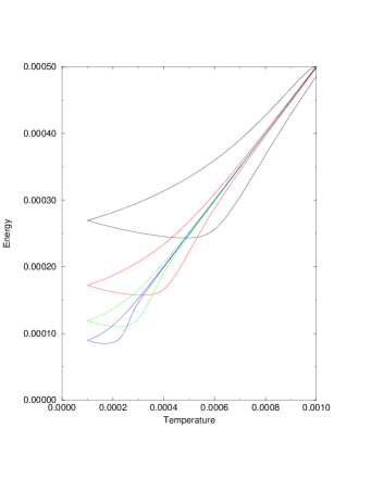
FIG. 1.: Cooling experiment. Values of the energy when we decrease and increase the temperature of the system at different ratios. From top to bottom, ratios 0.1,0.01,0.001 and 0.0001.

At very low temperatures the harmonic oscillator wants to relax to a configuration of very small entropy (indeed, because the oscillator is classical, the entropy diverges like $log(T)$ at low temperatures). In this situation the oscillator spends the major part of time looking for the ground state configuration. In some sense, the dynamics generates itself entropy barriers in a single potential well. This means that if we perform a cooling experiment, decreasing and increasing the temperature at a fixed rate, we expect that the system fails to relax to the equilibrium energy (see figure 1). This is a typical feature of glassy systems.

Let us consider the evolution of the energy at zero temperature. In this case, only those changes $\{\delta x_{i}\}$ which decrease the energy are accepted. Close to the equilibrium point $x=0$ the system will relax very slowly, mainly because the largest part of the movements are rejected. The relaxation of the energy at zero temperature is given by,

$$\frac{\partial E}{\partial t}=-(\frac{KE\Delta^{2}}{\pi})^{\frac{1}{2}}\exp(-\alpha^{2})\,+\,\frac{K\Delta^{2}}{4}\mathop{\operator@font erfc}\nolimits(\alpha)$$ (22)

To obtain the long time behavior we expand the error function in the limit $\alpha\to\infty$,

$$\frac{\partial E}{\partial t}=-\bigl{(}\frac{64}{\pi K\Delta^{2}}\bigr{)}^{\frac{1}{2}}E^{\frac{3}{2}}\exp(-\frac{K\Delta^{2}}{16E})$$ (23)

We should note that previous equation is extremely similar to that derived in the Monte Carlo dynamics of the Sherrington-Kirkpatrick spherical model in the adiabatic approximation at zero temperature. In terms of the parameter $\alpha$ (defined after eq.(6)) the equation (23) can be written in the simple form,

$$\frac{\partial\alpha}{\partial t}=\frac{\exp(-\alpha^{2})}{\sqrt{\pi}}~{}~{}~{}~{}.$$ (24)

For large times, the parameter $\alpha$ grows logarithmically in time,

$$\alpha(t)\simeq\bigl{(}\log(\frac{2t}{\sqrt{\pi}})+\frac{1}{2}\log(\log(\frac{2t}{\sqrt{\pi}})\bigr{)}^{\frac{1}{2}}$$ (25)

the acceptation rate eq.(10) decays like

$$A(t)\simeq\frac{1}{4t\log(\frac{2t}{\sqrt{\pi}})}$$ (26)

plus subdominant logarithmic corrections. The energy also decays logarithmically in time

$$E(t)\simeq\frac{K\Delta^{2}}{16}\frac{1}{\log(\frac{2t}{\sqrt{\pi}})+\frac{1}{2}\log(\log(\frac{2t}{\sqrt{\pi}}))}$$ (27)

Similarly the correlation function satisfies the equation,

$$\frac{\partial C(t,t^{\prime})}{\partial t}=-\bigl{(}\frac{K\Delta^{2}}{4\pi}\bigr{)}^{\frac{1}{2}}\frac{C(t,t^{\prime})}{\sqrt{E(t)}}\exp(-\frac{K\Delta^{2}}{16E(t)})$$ (28)

The same equation is fulfilled for the response function. Using the asymptotic differential equations for the energy (23), the correlation (28) and the response function, we can show that the correlation function for long times displays a solution of the type $C(t,t^{\prime})\simeq\frac{2E(t^{\prime})}{K}\frac{g(t)}{g(t^{\prime})}$ and $G(t,t^{\prime})\simeq\frac{2\alpha(t^{\prime})}{\sqrt{\pi}K}g(t)$, being $g(t)=\exp(-\alpha^{2})$. Using the asymptotic expression for the energy (27) we get,

$$C_{norm}(t,t^{\prime})=\frac{C(t,t^{\prime})}{2E(t^{\prime})/K}\simeq\frac{t^{\prime}}{t}\Bigl{(}\frac{\log(\frac{2t^{\prime}}{\sqrt{\pi}})}{\log(\frac{2t}{\sqrt{\pi}})}\Bigr{)}^{\frac{1}{2}}$$ (29)

$$G(t,t^{\prime})\simeq\frac{1}{Kt}\Bigl{(}\frac{\log(\frac{2t^{\prime}}{\sqrt{\pi}})+\frac{1}{2}\log(\log(\frac{2t^{\prime}}{\sqrt{\pi}}))}{\log(\frac{2t}{\sqrt{\pi}})}\Bigr{)}^{\frac{1}{2}}$$ (30)

FIG. 2.: Correlation function for different waiting times. From top to bottom, $t^{\prime}=3\cdot 10^{5}$,$1\cdot 10^{5}$,$1\cdot 10^{4}$,$1\cdot 10^{3}$. The short lines show the calculated asymptotic behavior eq(29)

This approximation is valid in the asymptotic limit of large values of $t^{\prime}$. The normalized correlation function shows aging behavior with a simple scaling form $t^{\prime}/t$ plus some logarithmic corrections. Apparently the response function (30) does not show aging because it does not depend on a ratio of functions depending on $t$ and $t^{\prime}$. But this is an artifact of the normalization factor necessary to make the response function to take a finite value at equal times. In fact, the leading behavior of the response function decays to zero for large values of $t$ and an appropriate normalization of the response function at equal times is necessary (in the same way as has been done for the correlation function). Note that for Langevin dynamics the normalization of the response function is not necessary since the $G(t,t^{\prime})$ at equal times already takes a finite value by definition (e.g., $\lim_{t^{\prime}\rightarrow(t)^{-}}G(t,t^{\prime})=1$). The normalized response function takes the simpler form,

$$G_{norm}(t,t^{\prime})=\frac{G(t,t^{\prime})}{G(t^{\prime}+0,t^{\prime})}\simeq\frac{t^{\prime}}{t}\Bigl{(}\frac{\log(\frac{2t^{\prime}}{\sqrt{\pi}})}{\log(\frac{2t}{\sqrt{\pi}})}\Bigr{)}^{\frac{1}{2}}$$ (31)

which displays aging with the same leading behavior as the normalized correlation function. We can obtain information about the dynamics (and in particular, about the response function) from the remanent magnetization [11]. In the present model the magnetization corresponds to the average position of the ensemble of oscillators (defined after (12)). The main equations (6),(13) and (14) have been derived in the absence of external field and starting with zero initial magnetization. In this case it is natural to compute the zero-field cooled magnetization. In this procedure the system is suddenly cooled down to a given temperature and after a waiting time $t_{w}$ a small step field $h(t^{\prime})=h\Theta(t^{\prime}-t_{w})$ is applied. If the value of $h$ is small enough then we are in the linear response regime. The magnetization starts to grow according to the relation,

$$M_{ZFC}=\int_{-\infty}^{t}G(t,t^{\prime})h(t^{\prime})dt^{\prime}=$$ (32)

$$=h\int_{t_{w}}^{t}G(t,t^{\prime})dt^{\prime}=hI(t_{w},t)$$ (33)

The quantity $I(t_{w},t)=\int_{t_{w}}^{t}G(t,t^{\prime})dt^{\prime}$ defines the integrated response function. From the exact expression obtained for the response function (16) we get, for the integrated response function,

$$I(t_{w},t)=\frac{1}{K}\bigl{(}1-\exp(-\int_{t_{w}}^{t}f(t^{\prime})dt^{\prime})\bigr{)}$$ (34)

In the large time limit $t\to\infty$ the zero-field cooled magnetization converges to its equilibrium value, the field-cooled magnetization $M_{FC}$. It is easy to check, from (33), (34) that $M_{FC}$ is given by $M_{FC}=\frac{h}{K}$, ie, the equilibrium linear magnetic susceptibility $\chi_{0}=M_{FC}/h=\frac{1}{K}$ is independent of the temperature.

Another interesting quantity to be calculated is the anomaly in the response function [12], defined as,

$${\bar{\chi}}\equiv\lim_{t\rightarrow\infty}\int_{0}^{t}dt^{\prime}G(t,t^{\prime})-\int_{0}^{\infty}G_{eq}(\tau)d\tau$$ (35)

$$=\lim_{t\rightarrow\infty}I(0,t)-\chi_{0}$$ (36)

$$=-\frac{1}{k}e^{-\int_{0}^{t}f(t^{\prime})dt^{\prime}}$$ (37)

$$G_{eq}(\tau)=\lim_{t_{w}\rightarrow\infty}G(t_{w},t_{w}+\tau)$$ (38)

For a finite value of $\beta$, the system decays to equilibrium in a finite time and for long times the integral $\int_{0}^{t}dt^{\prime}f(t^{\prime})$ behaves as $f_{eq}t$. This implies that the magnetization relaxes exponentially to zero, showing no aging for large values of $t_{w}$ and the ’anomaly’ relaxes exponentially to zero too. The behavior of the anomaly and the zero-field cooled magnetization is more interesting at zero temperature. In that case it can be shown that the leading behavior of the anomaly decays algebraically (as $1/Kt$) to zero. Using the asymptotic behavior of the energy eq.(27), it is easy to check that the zero-field cooled magnetization goes like,

$$\frac{M_{ZFC}}{M_{FC}}\simeq 1-\frac{t_{w}}{t}\Bigl{(}\frac{\log(\frac{2t_{w}}{\sqrt{\pi}})}{\log(\frac{2t}{\sqrt{\pi}})}\Bigr{)}^{\frac{1}{2}}$$ (39)

Using the linear response relation $M_{ZFC}+M_{TRM}=M_{FC}$ where $M_{TRM}$ is the thermo-remanent magnetization obtained by quenching the system in an (small) applied field and removing it at $t_{w}$, we get

$$\frac{M_{TRM}}{M_{FC}}\simeq\frac{t_{w}}{t}\Bigl{(}\frac{\log(\frac{2t_{w}}{\sqrt{\pi}})}{\log(\frac{2t}{\sqrt{\pi}})}\Bigr{)}^{\frac{1}{2}}~{}~{}~{}~{}~{}.$$ (40)

Both $M_{ZFC}$ and $M_{TRM}$ show aging with the leading $t/t_{w}$ scaling behavior. In figure 3 we show the thermo-remanent magnetization for the oscillator model for different values of $t_{w}$.

FIG. 3.: Thermo-remanent magnetization for different waiting times obtained from eq.(40). From left to right, $t_{w}=10$,$10^{2}$,$10^{3}$,$10^{4}$,$10^{5}$.

It has been suggested that the $X(t,t^{\prime})$ could be interpreted as an effective temperature [14, 15]. If we define $T_{f}(t^{\prime})=X(t,t^{\prime})/T$ then, from eq. (18), the fluctuation-dissipation theorem is obeyed with the effective temperature $T_{f}(t^{\prime})$. While this is a formal relation it would be interesting if the effective temperature derived in this way had some deep physical meaning. On the other hand, a well-founded physical interpretation of the violation of the fluctuation-dissipation relation, to our knowledge, does not exist. Note that it is possible to define different fluctuation-dissipation ratios (for instance, $X(t,t^{\prime})=-TG/\frac{\partial C}{\partial t}$) all giving $X(t,t^{\prime})=1$ in equilibrium. The definition here adopted is the conventional one which allows to obtain a closed expression for the integrated response function in case the function $X$ is solely function of the correlation $C(t,t^{\prime})$ [3, 4]. On general physical grounds one would expect an effective temperature larger than the temperature of the bath. To raise the temperature should contribute (by the equipartition theorem) those degrees of freedom which, during the process of relaxation towards the equilibrium, still are not frozen. For the simple model considered here such an interpretation seems to work. From equation (18) it can be shown that the effective temperature for a system relaxing at zero temperature is given by the relation $T_{f}(t^{\prime})\to 2E(t^{\prime})$. Consequently the effective temperature and the dynamical energy in the off-equilibrium regime are related by the thermodynamic relation suggesting that some kind of adiabatic theorem holds for this simple system in the long time limit. One can then ask if the whole time dependent probability distribution $p_{t}(\{x_{i}\})$ in the long-time limit is of the Boltzmann type but dependent on an effective temperature $T_{f}(t)$, i.e. $p_{t}(\{x_{i}\})\sim\exp(-E(\{x_{i}\})/T_{f}(t))$. It is easy to check that such a result is not possible [17] and equipartitioning is valid only for some finite moments of the probability distribution (for instance the second moment, i.e. the energy).

In conclusion, we have studied the Monte Carlo dynamics of an ensemble of linear harmonic oscillators. The extreme simplicity of this model makes it exactly solvable without loosing the interesting features of the non-equilibrium dynamics driven by entropic barriers. In this way, we are able to gather quite a lot of information and derive all relevant dynamical quantities with reasonable analytical effort.

We find a very slow relaxation near zero temperature, driven by a low acceptance rate, similar to that found in the Backgammon model [5], models of adsorption [18] as well as models for compaction of dry granular media [19]. In these cases, the origin of the slow relaxation is the existence of entropic barriers, although they are set up by different mechanisms. Note that the notion of entropic barrier or entropic trap is quite similar to the concept of effective volume in free volume theories. In our case this manifests as a inverse logarithmic law decay of the energy eq.(27) while in compaction of granular media this decay is found for the density of compaction. The model has also in common with models for glasses aging in the correlation function for long times. The correlation function $C(t,t^{\prime})$ presents a $\frac{t^{\prime}}{t}$ behavior with some logarithmic corrections (with $t^{\prime}$ the smallest time in the correlation function). It is interesting to note that this corrections appear also in the Backgammon model [16] (and presumably also in adsorption models [18] and models for compaction of dry granular media [19]) but do not appear in models with Langevin dynamics [20, 21]). We have found also aging in the magnetization (the integrated response function). This behavior appears associated to the algebraical decay of the ’anomaly’ as $t$ goes to infinity. Due to the zero value of the anomaly we expect a finite value of the overlap between two replicas [13] in the large $t$ limit if putted in the same configuration at $t_{w}$ (cloning procedure). This expectation stems from the simplicity of the landscape in this model (a single parabolic well). Consequently, this model falls into the first dynamical category (class I) proposed in [13]. However this model shares some features of the $p$-spin model (with $p>2$, belonging to class II) like aging in the integrated response function. Furthermore, this simple model lacks a fast process decaying to a plateau and also a two time dependence of the fluctuation-dissipation parameter, which only depends on the smallest time. This is probably due to the absence of a cooperative behavior.

Acknowledgments. We are grateful to S. Franz and Th. M. Nieuwenhuizen for a careful reading of the manuscript. The work by L.L.B. and F.G.P. has been supported by the DGES of Spain under grant PB95-0296. The work by F.R has been supported by FOM under contract FOM-67596 (The Netherlands).

REFERENCES

- [1] L. Lundgren, P. Svedlindh, P. Nordblad and O. Beckman, Phys. Rev. Lett. 51, 911 (1983); E. Vincent, J. Hammann and M. Ocio, in ‘Recent progress in Random Magnets’, ed. D. H. Ryan (Singapore: World Scientific) (1992), and references therein; L. C. E. Struik, Physical aging in amorphous polymers and other materials (Elsevier, Houston, 1978)
- [2] J. P. Bouchaud, L. F. Cugliandolo, J. Kurchan and M. Mézard, Out of Equilibrium dynamics in Spin Glasses and other Glassy systems Preprint cond-mat 9702070;
- [3] L. F. Cugliandolo and J. Kurchan, Phys. Rev. Lett. 71 173 (1993); J. Phys. A (Math. Gen.) 27 5649 (1994);
- [4] S. Franz and M. Mézard, Europhys. Lett. 26 209 (1994); Physica A 209 1 (1994);
- [5] F. Ritort, Phys. Rev. Lett 75, 1190 (1995); S. Franz and F. Ritort, Europhys. Lett. 31, 507 (1995); C. Godrèche, J. P. Bouchaud and M. Mézard, J. Phys. A (Math. Gen.)28 L603 (1995)
- [6] A. Barrat and M. Mezard, J. Physique I (France) 5 (1995) 941.
- [7] H. Rieger, J. Phys. A (Math. Gen.) L615 (1993);
- [8] N. G. Van Kampen, Stochastical Process in Physics and Chemistry North Holland (1981);
- [9] N. Metropolis, A. W. Rosenbluth, M. N. Rosenbluth, A. H. Teller and E. Teller, J. Chem. Phys. 21 1087 (1953);
- [10] L.L. Bonilla, F.G. Padilla, G. Parisi and F. Ritort Phys. Rev. B 54,6 , 4170 (1996); Europhys. Lett. 34 3 159 (1996);
- [11] E. Vincent, J. Hammann, M. Ocio, J.-P. Bouchaud and L. F. Cugliandolo, in Procceding of the Sitges Conference on glassy systems, June 1996, edited by M. Rubí, Preprint cond-mat 9607224;
- [12] S. Franz and M. Mézard, Physica A 210 48 1994;
- [13] A. Barrat, R. Burioni and M. Mézard, J. Phys. A (Math. Gen.) 29, 1311 (1996); A. Barrat, Ph. D. Thesis (Universite Paris VI), 1996.
- [14] S. Franz and F. Ritort, J. Phys. A (Math. Gen.) 30, L357 (1997).
- [15] L. F. Cugliandolo, J. Kurchan and L. Peliti, Phys. Rev E55, 3898 (1997).
- [16] C. Godrèche and J. M. Luck, J. Phys. A (Math. Gen.) 29 1915 (1996) and Preprint cond-mat 9707052
- [17] This result can be obtained for Langevin dynamics, S. Franz and F. Ritort (unpublished)
- [18] J. W. Evans, Rev. Mod. Phys. 65, 1281 (1993)
- [19] E. Caglioti, V. Loreto, H. J. Herrmann and M. Nicodemi, A “Tetris”-like model for the Compaction of dry granular media Preprint cond-mat 9705195.
- [20] S. Ciuchi and F. De Pascuale, Nucl. Phys. B 300, 31 (1988); L. F. Cugliandolo and D. S. Dean, J. Phys. A (Math. Gen.) 28, 213 (1995).
- [21] F.G. Padilla and F. Ritort, Langevin Dynamics of the Lebowitz-Percus Model, Preprint cond-mat 9703095 to appear in J. Phys. A.