CRITICAL EXPONENTS OF THE PURE AND RANDOM-FIELD ISING MODELS

Abstract

We show that current estimates of the critical exponents of the three-dimensional random-field Ising model are in agreement with the exponents of the pure Ising system in dimension $3-\theta$ where $\theta$ is the exponent that governs the hyperscaling violation in the random case.

The phase transition of Ising systems in a random quenched field is the subject of ongoing research[3]. It is known that in the three-dimensional case, there is a low-temperature ordered phase. This was originally suggested by a heuristic argument due to Imry and Ma[4] and has been shown rigorously[5, 6, 7]. In the presence of random fields, these arguments show in fact that the lower critical dimension is $d=2$ in the Ising case. The Hamiltonian of such systems is given by:

$$H=-\sum_{\langle ij\rangle}S_{i}S_{j}-\sum_{i}h_{i}S_{i}$$ (1)

where the Ising spins $S_{i}=\pm 1$ are on the sites of a $d$-dimensional cubic lattice and interact only between nearest-neighbors. The random fields $h_{i}$ have a quenched probability distribution $\overline{h}_{i}=0$ and $\overline{h_{i}h_{j}}={\overline{h}}\delta_{ij}$ where the overbar stands for average over the disorder. There is accumulating evidence for a second-order phase transition in three dimensions from Monte-Carlo studies[8, 9, 10], real-space renormalization group calculations[11, 12, 13] as well as series expansions[14].

The standard perturbative approach to critical phenomena leads to an upper critical dimension[15] $d=6$ for the random field problem and, below this dimension, the critical exponents are those of the pure Ising system in dimension $d-2$ within the $\epsilon=d-6$ expansion. In fact this dimensional reduction holds to all orders in perturbation theory[15, 16, 17, 18] in $\epsilon$. In view of the lower critical dimension $d=2$, this cannot be the whole story. More general renormalization group studies[19] have emphasized the role of a zero-temperature fixed-point ruling the physics at the transition point. This leads naturally to the presence of a new exponent $\theta$ that governs hyperscaling violation: $2-\alpha=\nu(d-\theta)$ where $\nu$ is the correlation length exponent and $\alpha$ the specific heat exponent. This general scheme is in agreement with the droplet picture of the transition[20, 21]. In these theories, there is no obvious relationship between the random-field exponents as a function of the dimension and the exponents of the pure Ising system in dimension $d-\theta$. Stated otherwise, the zero-temperature fixed point is a priori unrelated to the ordinary Ising fixed point. This implies also that there are a priori three independent exponents: $\theta$ is a new exponent unrelated to $\nu$ and $\eta$, the exponent of the decay of spin correlations at the critical point. However, it has been suggested that dimensional reduction is still valid[14, 22, 23] in a generalized form, i.e. $\theta=2-\eta$ so that a two-exponent scaling is again valid. This means that the exponents of the random-field Ising model in dimension $d$ would be those of the pure Ising model in dimension $d-\theta$.

In this Letter, we show that the best estimates for the critical exponents of the random-field Ising model in dimension $d=3$ are in fact in agreement with the exponents of the pure Ising model analytically continued in dimension $d^{\prime}=3-\theta$. This analytic continuation is obtained through effective summation methods of the perturbative $\epsilon=4-d^{\prime}$ expansion series for the critical exponents of the pure Ising system. Such a procedure has been explored in the past and leads to very stable estimates[24, 25].

The singular part of the free energy in a correlation volume $F_{\rm sing}$ is governed by the correlation length:

$$F_{\rm sing}\propto\xi^{\theta},$$ (2)

where the spin correlation length diverges at the critical point $\xi\propto|T-T_{c}|^{-\nu}$. This definition leads to a modified hyperscaling relation:

$$2-\alpha=\nu(d-\theta).$$ (3)

Right at the critical temperature, the decay of the connected spin correlation function can be written:

$$\overline{\langle S_{0}S_{x}\rangle-\langle S_{0}\rangle\langle S_{x}\rangle}\propto x^{-(d-2+\eta)}.$$ (4)

For the random field problem, the disconnected susceptibility has a different kind of scaling:

$$\overline{\langle S_{0}\rangle\langle S_{x}\rangle}\propto x^{-(d-4+\overline{\eta})}.$$ (5)

This defines the two exponents $\eta$ and $\overline{\eta}$. The general scaling theory of Bray and Moore[19] gives the following relation:

$$\theta=2-\overline{\eta}+\eta.$$ (6)

There is an exact inequality due to Schwartz and Soffer[26]:

$$\overline{\eta}\leq 2\eta,$$ (7)

which in fact appears to be fulfilled as an equality[4, 22, 14, 9]. The scaling relations between exponents for the pure Ising model in dimension $d^{\prime}$ are obtained from those for the random-field case in dimension $d$ through the relation:

$$d^{\prime}=d-\theta.$$ (8)

However, there is no direct evidence that the values of the exponents for the pure Ising model in dimension $d^{\prime}$ have any relationship with those for the random-field case in dimension $d$.

To explore the relationship with the critical properties of the pure Ising model, we have used the estimates of the exponents as a function of the dimension $d^{\prime}$ coming from the $\epsilon=4-d^{\prime}$ expansion, up to order $\epsilon^{5}$, of the pure system[25]. To extrapolate the series, one needs to use powerful summation techniques that have been widely studied in the past[27, 24, 25]. Let us explain here the principle of the procedure. If an exponent $E$ is known from the $\epsilon$-expansion:

$$E(\epsilon)=\sum_{k}E_{k}\,\,\epsilon^{k},$$ (9)

one has to construct the so-called Borel transform $B(\epsilon t)$:

$$E(\epsilon)=\int^{\infty}_{0}dt\,\exp(-t)\,t^{\rho}\,B(\epsilon t),$$ (10)

where $\rho$ is an adjustable parameter. The series expansion for the Borel transform is then given by:

$$B(\epsilon t)=\sum_{k}E_{k}\,(\epsilon t)^{k}/\Gamma(k+\rho+1),$$ (11)

where $\Gamma$ is Euler’s function. The coefficients $E_{k}$ are known to behave for large $k$ as $E_{k}\sim k!a^{k}k^{b}$ with some constants $a,b$. The advantage of the Borel transform is that this translates into a large $k$ behaviour $\sim a^{k}k^{b-\rho}$ for its coefficients in the series expansion. Thus the function $B(\epsilon t)$ is analytic at least in a circle: the closest singularity of $B(\epsilon t)$ occurs at $\epsilon t=-1/a$. Assuming that $B(\epsilon t)$ is analytic in the cut plane, one maps the cut plane onto a circle by use the mapping:

$$\epsilon t={4\over a}{w\over(1-w)^{2}}=\sum_{n}\lambda_{n}w^{n}.$$ (12)

The Borel transform is now given through a convergent series in $w$, which leads to

$$E(\epsilon)=\sum_{n}B_{n}\;(\int^{\infty}_{0}dt\,\exp(-t)\,t^{\rho}\,[w(t)]^{n}\,).$$ (13)

Apparent convergence of such an expression is improved by varying $\rho$ and by introducing other free parameters (see Ref.[25]). This leads to stable estimates of the exponent $E$ as a function of $\epsilon$. Errors in the extrapolation procedure can be estimated by varying the arbitrary parameters (like $\rho$) that enters the whole procedure.

Extrapolating down from $d^{\prime}=4$ to $d^{\prime}=2$, one finds for example $\nu=0.99(4)$ for the correlation length exponent and $\gamma=1.73(6)$ for the susceptibility exponent, in excellent agreement with the exact values from the Onsager solution $\nu=1$ and $\gamma=1.75$. As a consequence, it is best to pin the exponents to the exact values in $d^{\prime}=2$ by writing $E(\epsilon)=E(d^{\prime}=2)+(2-\epsilon){\tilde{E}}(\epsilon)$ and to perform then the above summation method on $\tilde{E}$. A global check of the method is provided by the comparison with other methods for $d^{\prime}=3$ : this scheme then leads for example to $\nu=0.6310(15)$ while the standard renormalization group result[27] from fixed dimension perturbation series is $\nu=0.6300(15)$, known to be in agreement with high temperature series and Monte-Carlo results.

Reliable critical exponents $\gamma,\nu,\beta,\eta$ of the pure system have thus been obtained as a function of the dimension $d^{\prime}$. In Figure 1, we plot the results for the susceptibility exponent $\gamma$. The best value is the central solid line while the two extremal solid lines define the errors (there is thus a collapse at $d^{\prime}=4$ and $d^{\prime}=2$ of the three lines). Between $d^{\prime}=4$ and $d^{\prime}=2$ the errors remain quite small and the value of the exponent does not vary very much. Below $d^{\prime}=2$, there is a rapid increase due to the proximity of the lower critical dimension of the pure problem.

We then consider the random-field Ising model in dimension $d=3$, for which reliable exponents are now available. The best Monte-Carlo results[9] are obtained using a binary distribution of random-field. From the corresponding estimates of the optimal run with ${\overline{h}}/T=0.35$, one has $\eta=0.56(3)$ and $\overline{\eta}=1.00(6)$, and one then obtains from eq.(8) and eq.(6): $d^{\prime}=1.44(10)$. The corresponding value for $\gamma$ is : $\gamma=2.3(3)$. These Monte-Carlo results for the random-field Ising model in dimension $d=3$ appear in Figure 1 as the solid box : its vertical size is fixed by the estimate of the exponent $\gamma$ with its error bar and its horizontal size is fixed by the range of $d^{\prime}$, which defines the solid box.

In Figure 1, the large intersection between the solid box and the domain between the extremal solid lines, as well as the good intersection of the central solid line, clearly shows that $\gamma$ of the three dimensional random problem is in agreement with $\gamma$ of the pure system for $d^{\prime}=3-\theta$, and in particular close to $\gamma$ of the pure system for $d^{\prime}\approx 1.5$ which corresponds to the simple guess[10] that random field fluctuations dominate the critical behaviour $F_{sing}\sim\xi^{d/2}$: $\theta=1.5$ in three dimensions.

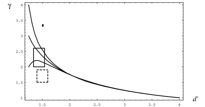
FIG. 1.: Critical exponent $\gamma$ of the magnetic susceptibility as a function of the dimension $d^{\prime}=3-\theta$. The meaning of the various symbols is given in the text.

We have also plotted in Figure 1 two less reliable other estimations: The dashed box is obtained in the same way as the solid one but with the results of the Monte-Carlo study of Ref.[10] using a Gaussian distribution of the random field, with a slower algorithm and a less extensive simulation than for the binary distribution. The two black dots are estimates from recent Migdal-Kadanoff renormalization-group studies[12, 13]. Other results coming from earlier Monte-Carlo simulations[28] $d^{\prime}=1.55(3)$ $\gamma=1.7(2)$, from real-space renormalization-group calculations[11] $\gamma=1.9\;-\;2.2$ or from high-temperature series expansion[14] $\gamma=2.1(2)$ have not been drawn on Figure 1 for clarity, since they are well compatible with the quoted Monte-Carlo results.

FIG. 2.: Critical exponent $\nu$ of the correlation length as a function of the dimension $d^{\prime}$. Same symbols as in Fig. 1

In Fig. 2, we plot the results for $\nu$ with the same symbols. The dashed line is the estimate (up to $d^{\prime}\approx 1.6$) coming from the near-planar interface model of Wallace and Zia[29] which has the same critical behaviour as the pure Ising model and can be expanded in powers of $\epsilon^{\prime}=d^{\prime}-1$, giving $\nu$ = $\epsilon^{\prime}{}^{-1}-1/2+\epsilon^{\prime}/2$ (We have plotted the only non-trivial Padé approximant). Note the agreement between this estimate and the $\epsilon=4-d^{\prime}$ expansion estimates.

FIG. 3.: Critical exponent $\beta$ of the magnetization as a function of the dimension $d^{\prime}$. Same symbols as in Fig. 1

In Fig. 3, we plot the order parameter exponent $\beta$. In this case, it is interesting to note that the Migdal-Kadanoff calculation[12, 13] shows a non-analytic vanishing of $\beta$ near $d=2$ and this also happens near $d^{\prime}=1$ in the droplet model of Bruce and Wallace[30] which is an extension of the near-planar interface model. Accordingly, our resummed results leads to an extremely small value (or even negative, the non-analytic behavior cannot be possibly reproduced by our approximants) of $\beta$ for the corresponding dimension.

FIG. 4.: Critical exponent $\eta$ of the spin correlations as a function of the dimension $d^{\prime}$. Same symbols as in Fig. 1

Finally, in Fig. 4, we plot $\eta$, again with the same symbols. In this case, as well as for $\beta$, the Monte-Carlo results are in good agreement with the Migdal-Kadanoff values.

The overall remarkable agreement clearly seen in our Figures between the results for the three dimensional random-field Ising model and those for the pure case for the corresponding dimension shows that the exponents of the random-field Ising model in three dimensions are in very good agreement with those of the pure Ising system in dimension $d^{\prime}=3-\theta$, and in particular very close to those of the pure system in dimension $\approx 1.5$ which corresponds to the a priori guess[10] $\theta=1.5$ in three dimensions.

We have thus obtained evidence for the generalized dimensional reduction for the random-field Ising model: the values of the exponents for the random model in dimension $d$ are in fact those for the pure case in dimension $d^{\prime}=d-\theta$.

- [1] Also at Université de Savoie and at Institut Universitaire de France.
- [2] URA 1436 du CNRS associée à l’Ecole Normale Supérieure de Lyon et à l’Université de Savoie.
- [3] T. Nattermann and J. Villain, Phase Transitions 11, 817 (1988); D. P. Belanger and A. P. Young, J. Mag. Mag. Mater. 100, 272 (1991).
- [4] Y. Imry and S. K. Ma, Phys. Rev. Lett. 35, 1399 (1975).
- [5] J. T. Chalker, J. Phys. C16, 6615 (1983).
- [6] D. S. Fisher, J. Fröhlich and T. Spencer, J. Stat. Phys. 34, 863 (1984).
- [7] J. Z. Imbrie, Phys. Rev. Lett. 53, 1747 (1984); Comm. Math. Phys. 98, 145 (1985); Physica A140, 291 (1986).
- [8] A. T. Ogielski and D. A. Huse, Phys. Rev. Lett. 56, 1298 (1986); A. T. Ogielski, Phys. Rev. Lett. 57, 1251 (1986).
- [9] H. Rieger and A. P. Young, J. Phys. A26, 5279 (1993) ; H. Rieger, Ann. Rev. Comput. Phys. 2, 296 (1995) (ed. D. Stauffer, World Scientific, Singapore). See also the values of the exponents quoted in Ref.[10].
- [10] H. Rieger, Phys. Rev. B52, 6659 (1995).
- [11] I. Dayan, M. Schwartz and A. P. Young, J. Phys. A26, 3093 (1993).
- [12] M. S. Cao and J. Machta, Phys. Rev. B48, 3177 (1993); A. Falicov, A. N. Berker and S. R. MacKay, Phys. Rev. B51, 8266 (1995).
- [13] J. Y. Fortin and P. C. W. Holdsworth, J. Phys. A29, L539 (1996).
- [14] M. Gofman, J. Adler, A. Aharony, A. B. Harris and M. Schwartz, Phys. Rev. Lett. 71, 1569 (1993).
- [15] G. Grinstein, Phys. Rev. Lett. 37, 944 (1976).
- [16] A. Aharony, Y. Imry and S. K. Ma, Phys. Rev. Lett. 37, 1364 (1976).
- [17] A. P. Young, J. Phys. C10, L257 (1977).
- [18] G. Parisi and N. Sourlas, Phys. Rev. Lett. 43, 744 (1979).
- [19] A. J. Bray and M. A. Moore, J. Phys. C18, L927 (1985).
- [20] J. Villain, J. Phys. (Paris) 46, 1843 (1985).
- [21] D. S. Fisher, Phys. Rev. Lett. 56, 416 (1986).
- [22] M. Schwartz, J. Phys. C18, 135 (1985).
- [23] Y. Shapir, Phys. Rev. Lett. 54, 154 (1985).
- [24] J. C. Le Guillou and J. Zinn-Justin, J. Phys. (Paris) 46, L137 (1985).
- [25] J. C. Le Guillou and J. Zinn-Justin, J. Phys. (Paris) 48, 19 (1987).
- [26] M. Schwartz and A. Soffer, Phys. Rev. Lett. 55, 2499 (1985).
- [27] J. C. Le Guillou and J. Zinn-Justin, Phys. Rev. Lett. 39, 95 (1977); Phys. Rev. B21, 3976 (1980); J. Phys. (Paris) 50, 1365 (1989).
- [28] A. P. Young and M. Nauenberg, Phys. Rev. Lett. 54, 2429 (1985).
- [29] D. J. Wallace and R. K. P. Zia, Phys. Rev. Lett. 43, 808 (1979).
- [30] A. D. Bruce and D. J. Wallace, Phys. Rev. Lett. 47, 1743 (1981); J. Phys. A16, 1721 (1983).