Domain Dynamics of Magnetic Films with Perpendicular Anisotropy

Abstract

We study the magnetic properties of nanoscale magnetic films with large perpendicular anisotropy comparing polarization microscopy measurements on $\mbox{Co}_{28}\mbox{Pt}_{72}$ alloy samples based on the magneto-optical Kerr effect with Monte Carlo simulations of a corresponding micromagnetic model. In our model the magnetic film is described in terms of single-domain magnetic grains, interacting via exchange as well as via dipolar forces. Additionally, the model contains an energy barrier which has to be overcome in order to reverse a single cell and a coupling to an external magnetic field. Disorder is taken into account.

We focus on the understanding of the dynamics especially the temperature and field dependence of the magnetisation reversal process. The experimental and simulational results for hysteresis, the reversal mechanism, domain configurations during the reversal, and the time dependence of the magnetisation are in very good qualitative agreement. The results for the field and temperature dependence of the domain wall velocity suggest that for thin films the hysteresis can be described as a depinning transition of the domain walls rounded by thermal activation for finite temperatures.

75.60.Ch, 75.60.Ej, 75.40.Mg

I Introduction

In recent years great effort was focused on the magnetisation reversal process in magnetic thin films with perpendicular anisotropy because of their potential application as high density recording media. In particular CoPt alloy films were found to be a very promising compound for magnetic and magneto-optic storage [1].

Two different mechanisms can be thought of to dominate the reversal process: either nucleation or domain wall motion [2]. Which of these mechanisms dominates a reversal process depends on the interplay of the different interaction forces between domains with different magnetic orientation. In recent experiments on $\mbox{Co}_{28}\mbox{Pt}_{72}$ alloy films [3, 4] a crossover from magnetisation reversal dominated by domain growth to a reversal dominated by a continuous nucleation of domains was found depending on the film thickness which was varied from 10nm to 30nm. Correspondingly, characteristic differences for the hysteresis loops have been found. Similar results have been achieved by simulations of a micromagnetic model using zero temperature dynamics [3, 4] and Monte Carlo methods respectively [5].

It is the goal of this paper to work out the relation between experiments and simulations. An exact, quantitative description of the experimental results is hindered by the facts that the observable length scales in experiment and simulation are different and that there is no straight forward mapping of the time scale of a Monte Carlo simulation on experimental time scales. However, the emphasis of our work is on a deeper qualitative understanding of the dynamical aspects of the magnetization reversal and especially on the principal influence of the field and the temperature on the domain wall velocity. We find that for thin films these dynamics is governed by a depinning transition of the domain walls rounded by thermal activation for finite temperatures.

II Experimental Methods

The CoPt alloy films were prepared under UHV conditions at low deposition rates on Si substrates covered with a 20nm Pt buffer layer. In order to achieve a dominant perpendicular anisotropy the films were grown at rather high substrate temperatures of about $220^{\circ}$C. The composition of 28 at.% Co and 72 at.% Pt is known to exhibit the maximum of the polar Kerr rotation for the whole range of alloys [1]. Structural characterization reveals a predominant fcc(111) texture. The films were usually found to form a polycrystalline microstructure. Scanning tunneling microscopy was used to determine the average grain size. The preparation process yields rather uniform grain size of the order of 20nm almost independent of the film thicknesses, which cover the range of 5 to 50nm.

X-ray analysis reveals a dispersion of the crystalline c-axis in the range of about 3 degrees. For the magnetic characterization we applied magneto-optic Kerr microscopy at very high spatial resolution of about 1$\mu$m [4]. The typical Kerr rotation for the CoPt alloy films is ranging from $0.1^{\circ}$ to $0.3^{\circ}$. High speed image processing technique using a low noise CCD camera is able to acquire domain patterns with millisecond time resolution. The experimental setup permits to gain complete hysteresis loops with applied external magnetic field up to 0.5T. An electrical heater assembly provides the variation of the sample temperature by direct heating using a bifilar heat wire. Image processing software was developed to determine the domain wall motion and the average magnetisation of the sample.

III Micromagnetic Model

$\mbox{Co}_{28}\mbox{Pt}_{72}$ alloy films have a polycrystalline structure. For a theoretical description by a micromagnetic model [6] the film is thought to consist of cells on a square lattice with a square base of size $L\times L$ where $L=20$nm. The height $h$ of the cells is varied from 10nm to 30nm. Due to the large anisotropy of the CoPt alloy film the cells are thought to be magnetised perpendicular to the film only with a uniform magnetisation $M_{s}$ which is set to the experimental value of $M_{s}=365$kA/m for the saturation magnetisation in these systems [7]. The cells interact via domain wall energy and dipole interaction. The coupling of the magnetisation to an external magnetic field $H$ is taken into account as well as an energy barrier which has to be overcome during the reversal process of a single cell.

From these considerations it follows that the change of energy caused by reversal of a cell $i$ with magnetisation $L^{2}hM_{s}\sigma_{i}$ with $\sigma_{i}=\pm 1$ and $\Delta\sigma=\sigma(new)-\sigma(old)=\pm 2$ is:

$$\Delta E_{i} = -\frac{1}{2}LhS_{w}\Delta\sigma_{i}\sum_{\langle j\rangle}\sigma_{j}$$ (3)

$$+\frac{\mu_{0}}{4\pi}M_{s}^{2}Lh^{2}\Delta\sigma_{i}\sum_{j}v(\sigma_{j},r_{ij})$$

$$-\mu_{0}HL^{2}hM_{s}\Delta\sigma_{i}$$

The first term describes the wall energy $\Delta E_{w}$ and the sum is over the four next neighbors. One can expect that the grain interaction energy density $S_{w}$ is a reduced Bloch-wall energy density $S_{B}$ since the crystalline structure of the system is interrupted at the grain boundary and also since there may be a chemical modulation of the CoPt alloy at the grain boundary. We varied the value of $S_{w}$ in the simulation and got the best agreement with experimental results for a value of $S_{w}=0.0022\mbox{J}/\mbox{m}^{2}$ which is approximately 50% of the Bloch-wall energy $S_{B}$ for this system [7].

In the second term describing the dipole coupling $\Delta E_{d}$ the sum is over all cells. $r_{ij}$ is the distance between two cells $i$ and $j$ in units of the lattice constant $L$. For large distances it is $v(\sigma_{j},r_{ij})=\frac{\sigma_{j}}{r_{ij}^{3}}$. For shorter distances a more complicated form which is a better approximation for the shape of the cells which we consider can be determined numerically and was taken into account.

The third term describes the coupling $\Delta E_{H}$ to an external field $H$.

Additionally, an energy barrier $\delta_{i}$ must be considered which describes the fact that a certain energy is needed to reverse an isolated cell. Two reversal mechanisms can be taken into account as limiting cases: (i) coherent rotation of the magnetisation vector described by an angel $\theta$: In this case the anisotropy leads to an energy barrier of $L^{2}hK_{u}$ where $K_{u}$ is the anisotropy constant which is $K_{u}=200\mbox{kJ}/\mbox{m}^{3}$ [7]. (ii) domain wall motion through the grain: In this case the energy barrier is $LhS_{b}$ due to the fact that the domain wall energy is lowered at the grain boundary. The highest possible value for $S_{b}$ is the Bloch-wall energy mentioned above but it can be assumed that the for the energy barrier relevant value is smaller than the value above since a Bloch wall is thicker than the size of the cell. Comparing these two energies for the reversal mechanism of a CoPt grain one finds that here domain wall motion through the grains has the lower energy barrier so that from now on only this mechanism will be taken into account. We assume that during the reversal process the energy barrier has its maximum value $LhS_{b}$ when the domain wall is in the center of the cell, i.e. when half of the cell is already reversed. Consequently, the energy barrier which has to be considered in a Monte Carlo simulation is reduced to $\delta=\max(0,LhS_{b}-\frac{1}{2}|(E_{w}+E_{d}+E_{H})|)$. The simulations are in good agreement with the experiments using $S_{b}=0.0007\mbox{J}/\mbox{m}^{2}$.

Note, that we have introduced two different wall energy densities, $S_{w}$ for the nearest neighbor interaction, and $S_{b}$ for the intrinsic energy barrier. They have the same physical origin but they have to be handled separately in our model: e. g., the limit of a system of isolated grains is described by $S_{w}\rightarrow 0$ but then there is still a finite $S_{b}$ due to the existence of energy barriers which are relevant for the flip of the isolated cells. The opposite limit is a system without grain boundaries. Here it is $S_{b}=0$, i. e., there is no energy barrier but the domain wall has still a constant, finite energy density $S_{w}$ which in this limit does not depend on the position of the wall.

Obviously, the grain sizes in the CoPt alloy are randomly distributed [3]. In order to be realistic, in our simulation disorder has to be considered (see also [8] for a discussion of the role of disorder in a similar simulation). In the model above this corresponds to a random distribution of $L$ which can hardly be simulated exactly since it modulates the normalized cell distance $r_{ij}$ of the dipole interaction. Therefore, as a simplified ansatz to simulate the influence of disorder we randomly distribute $L$ in the energy term that describes the coupling to the external field. Here a random fluctuation of $L$ is most relevant, since this term is the only one scaling quadratically with $L$. In the simulations we use a distribution which is Gaussian with width $\Delta$ = 0.1. Through this kind of disorder our model is mapped on a random-field model. Other possible origins of disorder in the CoPt films are e. g. fluctuations of the easy axis of the grains or fluctuations of the saturation magnetisation. Interestingly these kinds of disorder would also predominantly influence the last term in Eq. 3 and hence can be gathered in the random field.

The simulation of the model above was done as in earlier publications [5, 8] via Monte Carlo methods [9] using the Metropolis algorithm with an additional energy barrier. Since the algorithm satisfies detailed balance and Glauber dynamics it allows the investigation of thermal properties as well as the investigation of the dynamics of the system. Note that in the limit of low temperatures the Monte Carlo algorithm passes into a simple energy minimization algorithm with single spin flip dynamics, so that also the case of zero temperature can be investigated.

The size of the lattice was typically $150\times 150$. The dipole interaction was taken into account without any cut-off or mean field approximation.

IV Hysteresis and the Reversal Mechanism

We start our analysis by comparing the hysteresis loop from simulations for $T=300$K, Fig. 1, with the corresponding experimental hysteresis loop for room temperature, see Ref. [3, 4].

FIG. 1.: Simulated hysteresis loops for a 30nm and a 10nm film at $T=300$K.

The qualitative agreement is very good. In both cases, experiment as well as simulation the hysteresis loop of the thin film is nearly rectangular. For the thicker film the loop has a finite slope, especially at the end of the hysteresis. This can be understood through the different reversal mechanisms. The reversal of the 10nm film is dominated by domain wall motion. Once a nucleus begins to grow the domain wall motion does not stop until the magnetisation has completely changed. For the 30nm film the enhanced dipolar forces stabilize a mixed phase which can be changed only by a further increase of the external field [3, 4, 5]. The reason for the enhanced influence of the dipolar forces can be seen in Eq.3 where the dipole term is the only term that scales quadraticly with the film thickness $h$ which means that the influence of the dipole coupling is neglectable for $h\rightarrow 0$ and on the other hand strongly growing with increasing film thickness.

Quantitatively, the agreement of the simulation with the experimental results is reasonable only for the 30nm film while the nucleation field is much to high for the simulation of the 10nm film. There are several possible reasons for this effect. First, the nucleation field which in the case of domain wall motion dominated reversal is the field where domain wall motion starts depends on the size and on the shape of the nucleus. In an experimental situation point-like defects which are not visible in the optical regime can act as nuclei while there is no such artificial nucleus in our simulation. Second, some of the parameters of our model like the disorder or the Bloch-wall energy which influences the prefactors in Eq.3 may depend on the film thickness. In our simulation, they are thought to be constant – for simplicity and since we do not have more information about the thickness dependence of these parameters. Third, the time scale at which a hysteresis loop is observed may play an important role. This time scale is a few minutes in the experiments and around 60000 MCS in the simulations. To our knowledge, there is no straight forward way to map Monte Carlo simulation time on realistic time scales so that the observation-time windows might be different in experiment and simulation leading to different nucleation fields. Changing the sweeping rates changes the nucleation fields due to thermal activation, experimentally as well as in simulations, but this does not change the qualitative behavior.

However, it is not the aim of our simulations to calculate the nucleation field accurately. Rather, the simulations are thought to contribute to a better understanding of the fundamental properties of the system, especially to a better understanding of the dynamics.

V Dynamics and Temperature Dependence

The different reversal mechanisms we mentioned in the previous section manifest themselves also in a change of the dynamical behavior. We focus on the reversal dynamics, i. e.  the time dependence of the magnetisation after a rapid change of the field to a value which destabilizes the initial direction of magnetisation. The corresponding experimental and simulational time dependences of the magnetisation are compared in Fig. 2. The time-axis is normalized to that time at which half of the system is reversed.

FIG. 2.: Magnetisation versus time from measurement, a), after a rapid change of the field to 19.33kA/m (10nm) and 13.29kA/m (30nm) and from simulations, b), after a rapid change to 260 kA/m (10nm) and 220 kA/m (30nm).

For the case of the thin films the (absolute) value of the reversed field is larger than the coercive field while for the thicker film in the experimental situation a value above the nucleation field but below the coercive field had to be chosen since for larger fields the reversal is to fast to be observed with this experimental technique. Consequently, the long time limit of the corresponding experimental curve is above -1. Apart from that the experimental results and the results from simulations agree.

For the case of the 30nm film, i. e. for the nucleation driven reversal there is a rapid change of the magnetisation at the beginning of the reversal process. This demonstrates that the reversal process is dominated by nucleation and not by domain growth processes. In the limit of a constant nucleation rate $R$ and no growth processes the change of the magnetisation can be expected to be exponential [11].

On the other hand for the case of domain growth the change of magnetisation is slow at the beginning. If a constant number of nuclei and a constant domain wall velocity $v$ is assumed, the magnetisation of the reversed domains grows quadratic in time as long as the domains are so small that they do not overlap, $M(t)-M_{0}\sim-(vt)^{2}$. Consequently, the central quantity of the magnetisation reversal driven by domain wall motion is the domain wall velocity. Therefore, in the following we will investigate in detail the dependence of the domain wall velocity on the driving field and the influence of the temperature. Hence from now on we restrict ourselves to the investigation of the 10nm film.

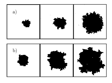
FIG. 3.: Domain image from MOKE measurements of a 10nm film 236, 313, and 468s after a rapid quench to a field of 17.7kA/m, a), and simulated domain configurations, of a $150\times 150$ system during the reversal of a 10nm film 10, 40, and 60 MCS after a rapid quench to a field of 245 kA/m, b)

For the determination of the domain wall velocity within the simulation we start with a system that has a nucleus of circular shape with a radius of 19 cells in the center of the $150\times 150$ system. When we switch on the driving field from the nucleus a domain starts to grow. For the better observation of the domain growth, in our flip-algorithm we do not consider cells that are not connected to the growing domain, i. e. we exclude the possibility of spontaneous nucleation. Otherwise we had – at least for finite temperatures – the problem that spontaneously new nuclei are build by thermal activation which with increasing radius overlap with the original domain. Fig. 3 illustrates the time development of a domain which follows from the method described above and compares it with experimental domain images. The black regions are reversed domains following the magnetic field. The domains look similar although their size is different (the linear size of the pictures is 3 $\mu$m in the simulation and 150$\mu$m experimental). This and also a more detailed analysis [12] leads to the conclusion that the domain walls are rough and hence self-similar (see [13] for a review on self similar interfaces). The shape of the domains is - within the simulations - influenced by the strength of the disorder. Note, however, that frozen disorder is not the only possible reason for the roughening of a domain wall. Other possible sources are the dipolar interactions as well as the dynamics of the model (see e.g. [14] for a discussion of the shape of domains in a model without disorder).

From both, the domain configurations from simulations and from experimental domain images the mean radius $r$ of the domains can be determined through the area $F$ of the reversed domain as $r=\sqrt{F/\pi}$, assuming that the domain has a circular shape. Additionally, the domain radius of the experimental domain images has been determined as the mean distance of the domain boundary from the center of the domain. Both definitions of $r$ lead to the same results.

Fig. 4a shows the time dependence of the radius measured at $T=299$K after a rapid change of the field to $H=17.7,18.0$, and $18.8$kA/m. Obviously, the domain wall velocity is constant and from the slope of the curves $v$ can be determined.

FIG. 4.: Measured radius of a domain versus time for $H=17.7,18.0,18.8$ kA/m. $T=299$K, a), and radius of the domain versus time from simulations for $H=225,230,235,240,245$ and zero temperature. The solid lines are best fitted.

In order to get a deeper understanding of the influence of the temperature on the dynamics apart from the “experimental temperatures” ($T\approx 300$K) we also simulated “extreme temperatures” ($T=0$K and $T=600$K). Fig. 4b shows - as an example - the $r(t)$ behavior from the simulations for $T=0$K and different fields. For the lowest field shown the domain wall is pinned, i. e. after a short period of rearrangement of the domain wall its movement stops and the radius remains constant. The pinning of the domain wall is due to energy barriers which follow from the disorder, the dipole field, and the intrinsic energy barrier of the single cell. For finite temperatures, the domain wall velocity is always finite (see discussion below).

For $r>150L/2=1.5\mu\mbox{m}$ the domain reaches the boundary of the system and - consequently - $r(t)$ saturates. For smaller $r$ the slope of the $r(t)$ curve is approximately constant and $v$ can be determined by fitting to a straight line. Fig. 5 shows the resulting dependence of the domain wall velocity on the driving field for $T=0,300$, and 600K.

FIG. 5.: Simulated domain wall velocity versus driving field for $T=600,300$, and 0K (from above). The solid lines are guides to the eye.

For zero temperature there is a sharp depinning transition [13] at a critical field $H_{c}$ from a pinned phase with $v=0$ to a phase with finite domain wall velocity. This transition can be interpreted in terms of a dynamic phase transition with $v\sim(H-H_{c})^{\theta}$ for $H>H_{c}$ where in our case the critical exponent is $\theta\approx 1$, a value which is the mean field result for a moving elastic interface [15] in a random-field. Also, this value has been observed in simulations of a soft spin model with random-fields [16]. Hence, it seems to be reasonable to consider the depinning transition we found to be in the universality class of a driven interface in the random-field Ising model. This fact is further confirmed by a dynamical scaling analysis of the structure of the domain walls in CoPt [12]. The central quantity in this analysis is the time dependent roughness of the domain wall which - following the theory of driven interfaces [13] - is characterized by a certain set of critical exponents. For the case of the CoPt alloy these exponents are also the same as those characterizing a driven interface in a random-field Ising model.

Note that in the models mentioned above the only origin for the depinning transition is the disorder. Here, the value of $H_{c}$ without disorder is zero. In our model, $H_{c}$ depends additionally on the dipole field and the intrinsic energy barrier of the single cell. A detailed analysis of these dependencies must be left for the future.

FIG. 6.: Scaling plot from Fig. 5.

For finite temperatures the transition is smeared since for finite temperatures there is even for $H<H_{c}$ for each energy barrier a finite probability that the barrier can be overcome by thermal fluctuations. Hence, for finite temperatures we expect a crossover from the dynamics of the zero temperature depinning transition explained above to a dynamics dominated by thermal activation where the corresponding waiting times are exponentially large. For $H<H_{c}$ the domain wall velocity should decrease like $\ln v\sim(H-H_{c})/T$. To illustrate this in Fig.6 we show the corresponding semi-logarithmic scaling plot. As we expect, the data for the two different finite temperatures collapse for $H<H_{c}$ on a straight line. For $H>H_{c}$ thermal activation is obviously less relevant since for these values of the driving fields even for zero temperature the domain walls move. Consequently, also for finite temperature but $H>H_{c}$ the domain wall dynamics is dominated by the zero temperature depinning transition, i.e. $v\sim H-H_{c}$.

FIG. 7.: Scaling plot for the measured domain wall velocities at $T=299,335,$ and $394$K.

Fig. 7 shows the same scaling plot for the experimental data. Obviously, all data are in the regime $H\ll H_{c}$, so that the scaling for thermal activation works. We are far away from the regime $H\approx H_{c}$ where the crossover to zero temperature depinning dynamics would start since from Fig. 7 it follows $H_{c}\approx 40$kA/m. There is no possibility for measurements at higher fields since for higher fields new domains build up spontaneously and overlap each other so that it is not possible to follow one single domain for the analysis of the domain wall velocity.

VI Conclusions

By comparing microscopy measurements on $\mbox{Co}_{28}\mbox{Pt}_{72}$ alloy samples based on the magneto-optical Kerr effect with Monte Carlo simulations we show that a micromagnetic model can be used for the understanding of magnetic properties of nanoscale magnetic films with high perpendicular anisotropy. The experimental and simulational results of the hysteresis, the reversal mechanism, the domain configurations during the reversal, the time dependence of the magnetisation and the temperature and field dependence of the domain wall velocity are in very good qualitative agreement.

For thin films the reversal is dominated by a growth of domains the dynamics of which can be described by the domain wall velocity. The results for the domain wall velocity suggest that for zero temperature the hysteresis can be understood as a depinning transition of the domain walls. For finite temperatures the transition is rounded by thermal activation and for fields smaller than the depinning field the domain wall movement is dominated by thermal activation.

REFERENCES

- [1] D. Weller, R. F. C. Farrow, J. E. Hurst, H. Notarys, H. Brändle, M. Rührig, and A. Hubert, Opt. Neural Networks 3(4), 353 (1994)
- [2] J. Pommier, P. Meyer, G. Pénissard, J. Ferré, P. Bruno, and D. Renard, Phys. Rev. Lett. 65, 2054 (1990)
- [3] T. Kleinefeld, J. Valentin, and D. Weller, JMMM 148, 249 (1994)
- [4] J. Valentin, T. Kleinefeld, and D. Weller, J. Phys. D, 29, 1111 (1996)
- [5] U. Nowak, IEEE Trans. Mag. 31, 4169 (1995)
- [6] W. Andrä, H. Danan, and R. Mattheis, Phys. Stat. Sol. (a), 125 , 9 (1991)
- [7] J. Harzer, RWTH Aachen, Ergebnisbericht (1992)
- [8] U. Nowak, U. Rüdiger, P. Fumagalli, and G. Güntherodt, Phys. Rev. B 54, 13017 (1996)
- [9] K. Binder and D. W. Heermann, Monte Carlo Simulations in Statistical Physics (Springer-Verlag, Berlin 1988)
- [10] R. D. Kirby, J. X. Shen, R. J. Hardy, and D. J. Sellmyer, Phys. Rev. B 49, 10810 (1994)
- [11] E. Fatuzzo, Phys. Rev. 127, 1999 (1962)
- [12] M. Jost and Th. Kleinefeld, submitted to Phys. Rev. B
- [13] M. Kardar and D. Ertas, in Scale Invariance, Interfaces, and Non-Equilibrium Dynamics, edited by A. McKane, M. Droz, J. Vannimenus, and D. Wolf, Plenum Press, New York 1995, pa. 89
- [14] A. Lyberatos, J. Earl, and R. W. Chantrell, Phys. Rev. B 53, 5493 (1996)
- [15] H. Leschhorn, J. Magn. Magn. Mat. 104-107, 309 (1992)
- [16] K. D. Usadel and M. Jost, J. Phys. A26, 1783 (1993)