Persistent Current in the Ferromagnetic Kondo Lattice Model

Abstract

In this paper, we study the zero temperature persistent current in a ferromagnetic Kondo lattice model in the strong coupling limit. In this model, there are spontaneous spin textures at some values of the external magnetic flux. These spin textures contribute a geometric flux, which can induce an additional spontaneous persistent current. Since this spin texture changes with the external magnetic flux, we find that there is an anomalous persistent current in some region of magnetic flux: near $\Phi/\Phi_{0}=0$ for an even number of electrons and $\Phi/\Phi_{0}=1/2$ for an odd number of electrons.

. ]

I Introduction and Model

The Berry phase [1] plays important roles in transport in mesoscopic systems. The most well known effect is the persistent current in quasi-one-dimensional normal-metal mesoscopic rings threaded with magnetic flux [2, 3]. This purely quantum effect manifests itself through the acquisition of a phase factor proportional to the magnetic flux which can change the boundary condition of the orbital wavefunctions [4]. Similarly, when a quantum spin adiabatically follows a magnetic field varying in space or time, the phase of its wavefunctions acquires an additional contribution – a geometric or Berry phase. It was shown by Loss et al. that this geometric phase can also induce persistent spin and mass currents [5].

In this paper, we study the persistent current in the 1D ferromagnetic Kondo lattice model (FKL) in the strong coupling limit. The FKL model in the strong coupling limit is related to the double exchange mechanism [6], which has been studied recently [7, 8, 9, 10, 11, 12, 13] due to its relevance to the colossal magnetoresistive Mn-oxides [14]. From now on, we will call the FKL model in the strong coupling limit the double exchange model. In this double exchange model, the ground state has spin textures at some values of magnetic flux [8, 13]. Since the electronic spins are strongly ferromagnetically coupled to the local spins, the spin texture of the local spin can induce a Berry phase in the electronic wavefunctions. The geometric flux produced by the local spin texture then induces spontaneous persistent currents. In previously studied persistent currents induced by geometric flux [5], the geometric Berry phase is due to adiabatically varying external magnetic field textures. In the double exchange model, the geometric Berry phase is due to the local spin textures, which depend self-consistently on the dynamics of the electrons. With the change of external magnetic flux, the local spin texture varies. This in turn will change the geometric phase-induced persistent current.

Here we study the zero temperature persistent current of an ideal one-channel double exchange ring threaded with a magnetic flux $\Phi$. The effects of finite temperature and disorder (elastic scattering) for double exchange systems are similar to those of the conventional persistent current in normal metal rings [15], and will not be considered here. The FKL model for a $N$-site 1D ring with magnetic flux $\Phi$ can be written as

$$H=-t\sum_{j,\sigma}\Bigl{(}e^{-{i2\pi\Phi\over N\Phi_{0}}}c_{j\sigma}^{\dagger}c_{j+1\sigma}^{\phantom{\dagger}}+h.c.\Bigr{)}$$ (1)

$$-{J_{H}\over 2}\sum_{i,\sigma,\sigma^{\prime}}c_{i\sigma}^{\dagger}({\vec{\sigma}})_{\sigma\sigma^{\prime}}^{\phantom{\dagger}}c_{i\sigma^{\prime}}^{\phantom{\dagger}}\cdot{\vec{S}}_{i},$$ (2)

where $\Phi_{0}=hc/e$, $\vec{\sigma}$ is the Pauli matrix, and $\vec{S}_{i}$ is the local spin. The operators $c_{i\sigma}^{\phantom{\dagger}}$ ($c_{i\sigma}^{\dagger}$) annihilate (create) a mobile electron with spin $\sigma$. For the double exchange model, $J_{H}/t\gg 1$. The zero temperature persistent current is equal to [4] $I=-c\partial E/\partial\phi$. It is easy to show that the free energy and persistent current are periodic in $\Phi/\Phi_{0}$. In Hamiltonian (2), we have neglected electron-electron interactions. In the double exchange model, the on-site electron-electron interaction is unimportant; it mainly renormalizes $J_{H}$.

In Sec. II, we will study the properties of spin textures and persistent current in the classical spin limit. In this limit, many results can be obtained analytically. In Sec. III, we study the effects of quantum fluctuations of order $1/S$ using a set of trial wavefunctions. In Sec. IV, we study the spiral ordering and persistent current for $S=1/2$ rings using exact diagonalization. We summarize our results in Sec. V.

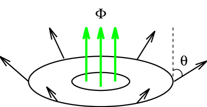
FIG. 1.: Local spin configuration with spiral ordering ${\hat{n}}_{j}=(\theta_{j},\phi_{j})=(\theta,j\phi_{0})$.

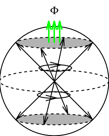
FIG. 2.: Two equivalent local spin configurations.

II Classical spin limit $S\rightarrow\infty$

The zero temperature persistent current is most easily calculable in the classical local spin limit. In this limit, the electrons are moving in a frozen local spin background. Hamiltonian (2) is then transformed to a one-body Hamiltonian. The ground state of Hamiltonian (2) is the ground state with optimal static local spin configuration. Since the original Hamiltonian is translation invariant and there is an effective short range ferromagnetic coupling between local spins due to the double exchange mechanism [6], we conjecture that the ground state has spiral ordering

$${\hat{n}}_{j}=(\theta_{j},\phi_{j})=(\theta,j\phi_{0}),$$ (3)

where $\phi_{0}=2m\pi/N$ is an integral multiple of $2\pi/N$ [see Fig. 1]. Note that the maximally polarized ferromagnetic ordering is an extreme case of this “spiral ordering” with $\theta=0$. Here $\theta$ is a variational parameter. We need to minimize the total energy $E_{tot}(\theta)$ to find the optimal $\theta$ for the local spin configurations.

Using the local spin configurations of Eq.(3), the Hamiltonian in $k$-space is

$$\tilde{\cal H}=\left(\begin{array}[]{lr}-{SJ_{H}\over 2}-T_{1}&V_{\delta}\\ V_{\delta}&{SJ_{H}\over 2}-T_{2}\end{array}\right)\,,$$ (6)

where $V_{\delta}=\Delta_{k}\sin\theta$, $\Delta_{k}=t\cos(k-\phi_{0}-{2\pi\Phi\over N\Phi_{0}})-t\cos(k-{2\pi\Phi\over N\Phi_{0}})$; $T_{1}=\epsilon^{0}_{k}-\Delta_{k}\cos\theta$ and $T_{2}=\epsilon^{0}_{k}+\Delta_{k}\cos\theta$ are the kinetic energies with $\epsilon^{0}_{k}=t\cos(k-{2\pi\Phi\over N\Phi_{0}})+t\cos(k-\phi_{0}-{2\pi\Phi\over N\Phi_{0}})$. From Eq.(6), we can show that the electronic energies with the two spin configurations $\theta\leftrightarrow\pi-\theta$, $\phi_{0}\leftrightarrow-\phi_{0}$ are degenerate [see Fig. 2].

The lower eigenenergy of the single electron states are

$$\epsilon_{k}=-\epsilon^{0}_{k}-\sqrt{({SJ_{H}\over 2})^{2}+\Delta_{k}^{2}-\Delta_{k}SJ_{H}\cos\theta}.$$ (7)

For $SJ_{H}\gg|\Delta_{k}^{2}|$,

$$\epsilon_{k}\simeq-{SJ_{H}\over 2}-\epsilon^{0}_{k}+\Delta_{k}\cos\theta-\Delta_{k}^{2}\sin^{2}\theta/(SJ_{H}).$$ (8)

Note that the eigenenergy is periodic in $\Phi/\Phi_{0}$.

In the limit $S=\infty$, the many-body wavefunction is just the Slater determinant of single particle wavefunctions. The total energy is

$$E_{tot}(\theta)=\sum_{|k|\leq k_{f}}\epsilon_{k}.$$ (9)

At zero flux $\Phi/\Phi_{0}=0$, the ground state for an even number of electrons has spiral spin ordering[13] $\theta=\pi/2$, i.e. the spins lie on the equator with zero total magnetization. For densities not close to half filling $n=N$ ($n/N\lesssim 0.8$ for $SJ_{H}\sim 12t$), the lowest energy spiral state has a single twist: $\phi_{0}=2\pi/N$. Actually, with zero flux, all the spiral states with finite $\theta$ and a single twist have lower energy than the lowest ferromagnetic state ($\theta=0$). The energy difference is:

$$E_{tot}(\theta)-E_{tot}(0)\simeq-\sin^{2}\theta/(SJ_{H})\sum_{|k|\leq k_{f}}\Delta^{2}_{k}$$ (10)

for $SJ_{H}\gg|\Delta_{k}^{2}|$. The results for an odd number of electrons is similar but shifted by $\Phi/\Phi_{0}\rightarrow\Phi/\Phi_{0}+1/2$. Here the Berry phase plays an important role to lower the energy of spiral states: with the spiral spin texture, the magnitude of the effective hopping is reduced, but the effective hopping matrix element has an additional complex phase, which can lower the total energy of spiral states for even (odd) number of electrons at $\Phi/\Phi_{0}=0$ ($\Phi/\Phi_{0}=1/2$).

Let us consider what happens if there is an infinitesimal external flux ${\Phi\over\Phi_{0}}\ll 1$. For $SJ_{H}\gg|\Delta_{k}^{2}|$,

$$E_{tot}(\theta)-E_{tot}(0)\simeq 2(1-\cos\theta)t\sin k_{f}\sin({2\pi\Phi\over N\Phi_{0}})$$ (11)

$$-\sin^{2}\theta/(SJ_{H})\sum_{|k|\leq k_{f}}\Delta^{2}_{k}.$$ (12)

Thus for small external flux ${\Phi\over\Phi_{0}}\ll 1$, the spiral angle $\theta$ decreases as

$$\cos\theta\propto\sin({2\pi\Phi\over N\Phi_{0}}),$$ (13)

and we can expect that as the magnetic flux $\Phi/\Phi_{0}$ changes, the pitch of the spiral ordering remains constant (i.e. $\phi_{0}=2\pi/N$), and the angle $\theta$ of the spiral ordering decreases continuously. At some critical value $\Phi=\Phi_{c}$, $\theta=0$, i.e. the spins become ferromagnetically ordered. In Fig. 3, we show the change of spiral ordering angle $\theta$ with magnetic flux.

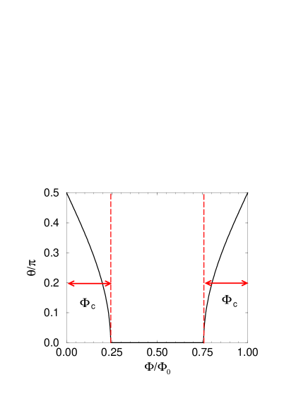
FIG. 3.: Change of the spiral ordering angle $\theta$ with magnetic flux $\Phi/\Phi_{0}$ at $SJ_{H}=12t$ and $S=\infty$ for a $N=450$ ring with $n=300$.

At fixed density, the critical value of magnetic flux $\Phi_{c}$ depends only weakly on the size of the ring $N$, as shown in Fig. 4. From Fig. 4, we can see that the critical value increases slightly with increasing system size $N$ and saturates at $N\lesssim 10^{3}$. As shown in Fig. 5, $\Phi_{c}$ depends nearly quadratically on the electron density. From this density dependence, we can also see that there is no particle-hole symmetry in this model. Since at half filling $n=N$ the ground state is antiferromagnetically ordered, our calculations are not valid close to half-filling. We also show the $SJ_{H}$ dependence of $\Phi_{c}$ in Fig. 6, from which we can conclude that it is very close to a power law for large $SJ_{H}$: $\Phi_{c}\sim C/(SJ_{H})$. This $1/(SJ_{H})$ dependence is expected from Eq. (12).

FIG. 4.: System size dependence of the critical magnetic flux $\Phi_{c}$ in the classical spin limit. $SJ_{H}=12t,24t$, density $\nu=2/3$.

FIG. 5.: Density dependence of the critical magnetic flux $\Phi_{c}$ in the classical spin limit. $SJ_{H}=12t$, $N=300$.

FIG. 6.: Hund’s rule coupling dependence of the critical magnetic flux $\Phi_{c}$ in the classical spin limit. $n=200$, $N=300$.

When the local spins are not ferromagnetically ordered, their spin texture will induce a Berry phase in the electron wavefunctions. Thus finite $\theta$ will induce a geometric flux, which in turn induces a spontaneous persistent current in the mesoscopic double exchange ring. This spontaneous persistent current will cancel part of the persistent current due to finite external magnetic flux. In Fig.(7), we show structures of the persistent current for even and odd numbers of electrons. In conventional mesoscopic systems, the zero temperature persistent current is linear in $\Phi$ for $k\Phi_{0}<\Phi<(k+1)\Phi_{0}$ for an even number of electrons, and $(k-1/2)\Phi_{0}<\Phi<(k+1/2)\Phi_{0}$ for an odd number of electrons. In a mesoscopic double exchange ring, due to the additional contribution to the persistent current from spin textures, the persistent currents are no longer monotonic in the regions mentioned above. Upon ensemble averaging of rings with different electron numbers, the period of the persistent current is changed from $\Phi=\Phi_{0}$ to $\Phi=\Phi_{0}/2$. For double exchange rings, the persistent current has anomalous regions near both $\Phi=\Phi_{0}$ and $\Phi=\Phi_{0}/2$ after ensemble averaging. In the remainder of this paper, we will continue to discuss even and odd numbers of electrons separately.

FIG. 7.: Persistent current in a double exchange ring in the classical spin limit: $N=450$, $n=300$ (solid line), and $n=301$ (dashed line), $SJ_{H}=16$. The dotted-dashed lines are the persistent currents in a conventional mesoscopic metallic ring.

III semiclassical spin limit $S\gg 1$

If the local spin $S$ is large but finite, the local spins have quantum fluctuations of order $1/S$, which can be taken advantage of by electrons to lower the electronic energy. This is the spin polaronic effect, which is similar to that in the Hubbard model [16]. Here we still consider the case where the ground state is either spirally ordered or ferromagnetically ordered, defined by ${\hat{n}}_{j}=(\theta_{j},\phi_{j})=(\theta,j\phi_{0})$, as in the classical limit.

First we consider the eigenstates of the single itinerant electron case. If one electron is at site $j$, the complete spin basis for this site can be chosen as

$$|S+{1\over 2},S+{1\over 2}\rangle,|S+{1\over 2},S-{1\over 2}\rangle,|S+{1\over 2},S-{3\over 2}\rangle,\cdots$$ (14)

$$|S-{1\over 2},S-{1\over 2}\rangle,|S-{1\over 2},S-{3\over 2}\rangle,|S-{1\over 2},S-{5\over 2}\rangle,\cdots$$ (15)

with a quantization axis of ${\hat{n}}_{j}$. In the semiclassical limit, these total spin states $|S\pm{1\over 2},S\pm{1\over 2}-k\rangle$ with the local quantization axis of ${\hat{n}}_{j}$ are an appropriate basis to describe the spin states at the site with the itinerant electron present. In the classical limit as studied in the previous section, only $|S\pm{1\over 2},S\pm{1\over 2}\rangle$ need be used to construct the exact wavefunctions. In the semiclassical limit, the quantum fluctuation corrections will come from the contributions of $|S\pm{1\over 2},S\pm{1\over 2}-k\rangle$ ($k>0$). If we include just the first order quantum fluctuation effects, we need a four trial wavefunction basis:

$$|\psi_{j}^{(1)}\rangle = |S+{1\over 2},S+{1\over 2}\rangle_{\displaystyle{\hat{n}}_{j}}^{\phantom{\displaystyle{\hat{n}}_{j}}}\otimes\{|S,S\rangle_{\displaystyle{\hat{n}}_{i\neq j}}^{\phantom{\displaystyle{\hat{n}}_{i\neq j}}}\}$$ (16)

$$|\psi_{j}^{(2)}\rangle = |S-{1\over 2},S-{1\over 2}\rangle_{\displaystyle{\hat{n}}_{j}}^{\phantom{\displaystyle{\hat{n}}_{j}}}\otimes\{|S,S\rangle_{\displaystyle{\hat{n}}_{i\neq j}}^{\phantom{\displaystyle{\hat{n}}_{i\neq j}}}\}$$ (17)

$$|\psi_{j}^{(3)}\rangle = |S+{1\over 2},S-{1\over 2}\rangle_{\displaystyle{\hat{n}}_{j}}^{\phantom{\displaystyle{\hat{n}}_{j}}}\otimes\{|S,S\rangle_{\displaystyle{\hat{n}}_{i\neq j}}^{\phantom{\displaystyle{\hat{n}}_{i\neq j}}}\}$$ (18)

$$|\psi_{j}^{(4)}\rangle = |S-{1\over 2},S-{3\over 2}\rangle_{\displaystyle{\hat{n}}_{j}}^{\phantom{\displaystyle{\hat{n}}_{j}}}\otimes\{|S,S\rangle_{\displaystyle{\hat{n}}_{i\neq j}}^{\phantom{\displaystyle{\hat{n}}_{i\neq j}}}\},$$ (19)

where $|\cdots\rangle_{\displaystyle{\hat{n}}_{i\neq j}}^{\phantom{\displaystyle{\hat{n}}_{i\neq j}}}$ is the spin state $|\cdots\rangle$ with the local quantization axis ${\hat{n}}_{j}$, which is a generalized coherent state [17] in the global quantization axis. Although we cannot show that the trial wavefunction basis in Eq.(19) rigorously describes the $1/S$ corrections to the results in the classical spin limit, we believe this will at least describe the qualitative effects of $1/S$ corrections. Note also that one can include a variational component in the empty sites wavefunctions such as $\{|S,S\rangle_{\displaystyle{\hat{n}}_{i\neq j}}^{\phantom{\displaystyle{\hat{n}}_{i\neq j}}}+c|S,S-1\rangle_{\displaystyle{\hat{n}}_{i\neq j}}^{\phantom{\displaystyle{\hat{n}}_{i\neq j}}}\}$, where $c$ is a variational parameter. But one can show that these corrections to the eigenenergy will be higher order in $1/S$ and thus negligible.

Using the variational basis (19), the Hamiltonian in $k$-space can be readily written down. For simplicity, we will only discuss the large Hund’s rule coupling limit $SJ_{H}=\infty$. Then we only need the basis states $|\psi_{j}^{(1)}\rangle$ and $|\psi_{j}^{(3)}\rangle$. The Hamiltonian in this variational $2\times 2$ basis is

$$\tilde{\cal H}=\left(\begin{array}[]{lr}-{SJ_{H}\over 2}-T_{1}&\sqrt{1\over 2S+1}V_{\delta}\\ \sqrt{1\over 2S+1}V_{\delta}&-{SJ_{H}\over 2}-T_{3}\end{array}\right)$$ (22)

where $T_{3}={1\over 2S+1}(\epsilon^{0}_{k}+\Delta_{k}\cos\theta)$.

From the above trial wavefunctions we can see that quantum fluctuations make the spins near the electron more polarized than the average spiral ordering direction. Thus we can think of the quantum fluctuation effect as a spin polaron effect. In the limit $J_{H}\rightarrow\infty$, the eigenenergies of the single electron states are

$$\epsilon_{k}=-{SJ_{H}\over 2}-{1\over 2}(\epsilon_{k}^{0}-\Delta_{k}\cos\theta+\delta)$$ (23)

(24)

$$-{1\over 2}\sqrt{(\epsilon_{k}^{0}-\Delta_{k}\cos\theta-\delta)^{2}+{4\over 2S+1}\Delta^{2}_{k}\sin^{2}\theta},$$ (25)

where $\delta={1\over 2S+1}(\epsilon_{k}^{0}+\Delta_{k}\cos\theta)$. When $|\epsilon_{k}^{0}-\Delta_{k}\cos\theta-\delta|\gg|2\Delta_{k}\sin\theta/|\sqrt{2S+1}$,

$$\epsilon_{k}=-{SJ_{H}\over 2}-\epsilon_{k}^{0}+\Delta_{k}\cos\theta-{\Delta^{2}_{k}\sin^{2}\theta\over 2S|\epsilon_{k}^{0}-\Delta_{k}\cos\theta-\delta|}\,.$$ (26)

In the semiclassical limit, we can construct approximate many-body wavefunctions using Slater determinants of single particle wavefunctions. However, this construction is only approximate because we neglect the interaction between different spin polarons. The corrections due to the spin polaron interaction is $O(n/S^{2})$. Thus this approximation is only valid for the dilute electron limit and large $S$. Similar to the finite $J_{H}$ effects, the quantum fluctuations induce a spiral ordering instability at $\Phi/\Phi_{0}=0$ for an even number of electrons and $\Phi/\Phi_{0}=1/2$ for an odd number of electrons. From Eq.(26), the lowering of the GS energy with spiral ordering due to quantum fluctuations is $E_{sp}-E_{FM}\propto-|t|/S$. Figure (8) show the persistent current for semiclassical spins. For low electron densities, the $1/S$ quantum fluctuation effects are similar to those of finite $SJ_{H}$ in the classical spin limit.

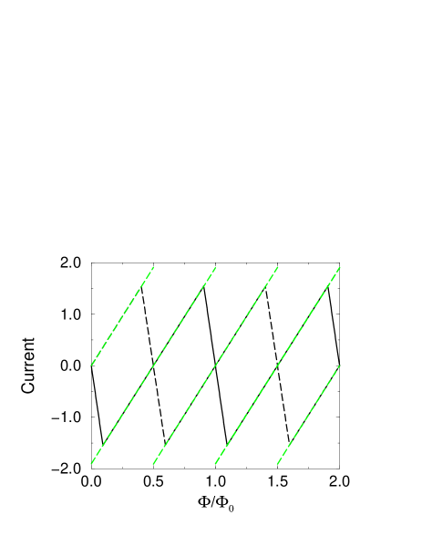
FIG. 8.: Persistent current in a double exchange ring in the semiclassical spin limit: $N=300$, $n=120$ (solid line), and $n=121$ (dashed line), $S=5$, $J_{H}=\infty$. The grey long-dashed lines are the persistent currents in a conventional mesoscopic metallic ring.

IV Persistent current in $S=1/2$ systems –exact diagonalization study

From the results in the classical and semiclassical limits, we expect that the spiral ordering instability will be enhanced in the quantum spin limit. This instability for general spin $S$ has been demonstrated previously [13] using a many-body trial wavefunction. To confirm that the ground state spin texture is indeed spiral for a quantum spin, we calculate the exact ground state for $S=1/2$ rings using exact diagonalization[13]. For an even number of electrons, we find that the ground state has total spin $S_{total}=0$ for both large $SJ_{H}$ and $SJ_{H}=\infty$ at $\Phi/\Phi_{0}=0$. With an increase of external flux, the total spin $S_{total}$ of the ground state increases, to $S_{total}=S^{max}\equiv(NS+n/2)$ at $\Phi/\Phi_{0}=1/2$. For an odd number of electrons, the results are shifted by $\Phi/\Phi_{0}\rightarrow\Phi/\Phi_{0}+1/2$. We speculate that the non-ferromagnetic state with $S_{total}<S^{max}$ is a sum over global rotations of spiral states with polarization angle $\theta$ ($0\leq\theta<\pi/2$). To check this statement numerically, we calculate the correlation function $\langle({\vec{S}}_{1}\times{\vec{S}}_{2})\cdot({\vec{S}}_{i}\times{\vec{S}}_{i+1})\rangle$ for even numbers of electrons at $\Phi/\Phi_{0}=0$. Because this ground state with $S_{total}=0$ can be thought of as a sum over all global rotations, we need to look at scalar correlation functions. The most relevant correlation function for the spiral ordering is $\langle({\vec{S}}_{1}\times{\vec{S}}_{2})\cdot({\vec{S}}_{i}\times{\vec{S}}_{i+1})\rangle$. In Fig.(9), we show the spiral correlation function $\langle({\vec{S}}_{1}\times{\vec{S}}_{2})\cdot({\vec{S}}_{i}\times{\vec{S}}_{i+1})\rangle$ for different size rings of spin $S=1/2$. The correlation is only weakly dependent on $i$ and has magnitude $\sim(0.25\sin(2\pi/N))^{2}$. This correlation function for $S=1/2$ is closer to $(0.25\sin(2\pi/N))^{2}$ as the system size N and/or electron number n increases. This clearly demonstrates that the spin ordering is spiral, similar to what we find in the classical and semiclassical limits.

The geometrical flux due to the local spin textures also contributes to the persistent currents in quantum spin systems. In Fig. (10), we show the exact diagonalization results for the persistent current in $S=1/2$ double exchange rings. We can see from Fig. (10) that the width of the anomalous region is increased compared to that in the classical [see Fig. (7)] and semiclassical limit [see Fig. (8)]. This demonstrates that the possibility of spiral spin ordering is enhanced in the quantum spin limit, as expected from the $1/S$ results. Although we do not have enough numerical results for $\Phi_{c}$ to study the dependences on system size $N$, electron density $n$, and $SJ_{H}$, we believe that these dependences will be similar to those for classical local spin double exchange rings, as shown in Figs.(4)-(6).

FIG. 9.: Correlation $\langle({\vec{S}}_{1}\times{\vec{S}}_{2})\cdot({\vec{S}}_{i}\times{\vec{S}}_{i+1})\rangle$ for $S=1/2$ rings normalized by $(0.25\sin(2\pi/N))^{2}$. $SJ_{H}=40t$.

FIG. 10.: Persistent currents in the $S=1/2$ double exchange system. N=6,8 and n=2,3. $SJ_{H}=40t$.

V Conclusion

In conclusion, we have studied the novel zero temperature persistent current in the double exchange system. In this system, there are spontaneous spin textures at some values of the external magnetic flux. These spin textures contribute a geometric flux, which can induce additional spontaneous persistent current. Since the spin textures vary with the change of external magnetic flux, there are anomalous persistent currents in the region near $\Phi/\Phi_{0}=0$ for an even number of electrons and $\Phi/\Phi_{0}=1/2$ for an odd number of electrons. After ensemble averaging of double exchange rings with different electron numbers, the persistent current has a period of $\Phi=\Phi_{0}/2$, and the anomaly occurs at $\Phi/\Phi_{0}=0$ and $1/2$. The effect of disorder (elastic scattering) and finite temperature for the double exchange systems are similar to those in conventional normal metal rings [15]. With the advance of fabrication technology, this fascinating anomalous persistent current and the magnetic flux dependent spin texture may become observable.

Acknowledgements: This work was conducted under the auspices of the US Department of Energy, and supported (in part) by funds provided by the University of California for the conduct of discretionary research by Los Alamos National Laboratory.

REFERENCES

- [1] M. V. Berry, Proc. Roy. soc. London A 392, 45 (1984).
- [2] M. Büttiker, Y. Imry, and R. Landauer, Phys. Lett. 96A, 365 (1983).
- [3] F. Block, Phys. Rev. 137, A787 (1965); 166, 415 (1968).
- [4] N. Byers and C. N. Yang, Phys. Rev. Lett. 7, 46 (1961).
- [5] D. Loss, P. Goldbart, and A. V. Balatsky, Phys. Rev. Lett. 65, 1655 (1990); D. Loss and P. Goldbart, Phys. Rev. B 45, 13544 (1992).
- [6] C. Zener, Phys. Rev. 82, 403 (1951); P . W. Anderson and H. Hasegawa, Phys. Rev. 100, 675 (1955). In the strong coupling limit, electronic spins will be parallel to local spins at every site to reduce the exchange coupling energy. The electrons hop more easily if the neighboring local spins are parallel. This is the double exchange mechanism proposed by Zener.
- [7] K. Kubo and N. Ohata, J. Phys. Soc. Jpn. 33, 21 (1972).
- [8] K. Kubo, J. Phys. Soc. Jpn. 51, 782 (1982).
- [9] A. J. Millis, P. B. Littlewood, and B. I. Shraiman, Phys. Rev. Lett. 74, 5144 (1995); A. J. Millis, R. Mueller, and B. I. Shraiman, Phys. Rev. B 54, 5405 (1996).
- [10] J. Inoue and S. Maekawa, Phys. Rev. Lett. 74, 3407, (1995).
- [11] H. Röder, J. Zang, A.R. Bishop, Phys. Rev. Lett. 76, 1356, (1996); J. Zang, A.R. Bishop, and H. Röder, Phys. Rev. B 53, R8840 (1996).
- [12] E. Müller-Hartmann and E. Dagotto, Phys. Rev. B 54, R6819.
- [13] J. Zang, H. Röder, A.R. Bishop, S.A. Trugman, J. Phys.: Cond. Matt. 9, L157 (1997).
- [14] G.H. Jonker and J.H. Van Santen, Physica 16, 337 (1950); ibid 19, 120 (1950); J. Volger, Physica 20, 49-66 (1954); E.D. Wollan and W.C. Koehler, Phys. Rev. 100, 545 (1955); R. von Helmholt et al, Phys. Rev. Lett. 71, 2331 (1993); S. Jin et al, Science, 264, 413 (1994).
- [15] H.F. Cheung et al. Phys. Rev. B 37, 6050 (1988).
- [16] J.R. Schrieffer, X.G. Wen, and S.C. Zhang, Phys. Rev. B 39, 11663 (1989).
- [17] See, for example, D.K. Sodickson and J.S. Waugh, Phys. Rev. B 52, 6467 (1995), and references therein.