Droplets nucleation, and Smoluchowski’s equation with growth and injection of particles

Abstract

We show that models for homogeneous and heterogeneous nucleation of $D$-dimensional droplets in a $d$-dimensional medium are described in mean-field by a modified Smoluchowski equation for the distribution $N(s,t)$ of droplets masses $s$, with additional terms accounting for exogenous growth from vapor absorption, and injection of small droplets when the model allows renucleation. The corresponding collision kernel is derived in both cases. For a generic collision kernel $K$, the equation describes a clustering process with clusters of mass $s$ growing between collision with $\dot{s}\propto s^{\beta}$, and injection of monomers at a rate $I$. General properties of this equation are studied. The gel criterion is determined. Without injection, exact solutions are found with a constant kernel, exhibiting unusual scaling behavior. For a general kernel, under the scaling assumption $N(s,t)\sim Y(t)^{-1}f(s/S(t))$, we determine the asymptotics of $S(t)$ and $Y(t)$, and derive the scaling equation. Depending on $\beta$ and $K$, a great diversity of behaviors is found. For constant injection, there is an asymptotic steady state with $N(s,t=\infty)\propto s^{-\tau}$ and $\tau$ is determined. The case of a constant mass injection rate is related to homogeneous nucleation and is studied. Finally, we show how these results shed some new light on heterogeneous nucleation with $d=D$. For $d=D=2$ (discs on a plane), numerical simulations are performed, in good agreement with the mean-field results.

I Introduction

Some very simple and practically important physical phenomena can be related to aggregation models, and as a consequence a host of experimental, numerical and theoretical studies are to be found in the literature. Classical fields of application are atmosphere sciences, material sciences, chemical engineering and cosmology, among others [friedlander77, family84, stanley86, vicsek92]. One of these phenomena is dropwise condensation on a substrate [meakindrop92], for instance water on a cold window pain, which bears on important implications in heat transfer engineering and material sciences, and generates fascinating droplets patterns, also called breath figures [beysens86]. Droplets grow from vapor, and when two droplets come into contact, they coalesce to form a bigger droplet, with mass (or volume) conservation. The underlying physics is rich, and it is not our purpose to fully discuss it here (see [meakindrop92]). Simple models have been introduced to describe the late stage of droplet growth and coalescence, of basically two kinds [meakindrop92, family88, family89, fritter91, derrida91, marcos95]. On the one hand, in heterogeneous nucleation models, one starts from a fixed number of nucleation sites (in physical situations these might be dust particles, substrate defects…). Droplets grow on these sites through vapor absorption, and when two neighboring droplets overlap, they coalesce to form a single droplet, thus reducing the number of droplets. On the other hand, in homogeneous growth models [family88], nucleation can occur anywhere on the substrate: some very small droplets are randomly deposited, which leads to the growth of existing droplets, and the creation of new small droplets if deposition occurs in a free zone.

Both kinds of models are aggregation models, with the unusual feature that the aggregating particles grow between coalescence events. Homogeneous growth has the additional feature that there is a source of small droplets, which relates this model to aggregation in presence of a source, which is also widely-studied in the literature [klett75, white82, crump82, hendriks85, vicsek85, racz85, hayakawa87, takayasu88, takayasu89, majumdar93]. Experiments and numerical simulations [meakindrop92, family89] show that the time dependent droplet mass distribution $N(s,t)$ ($s$ being the volume of the droplets), exhibits dynamic scaling, i.e. that for large times $N(s,t)\propto S(t)^{-\theta}f(s/S(t))$. $S(t)$ is a typical droplet mass (proportional to $<s^{2}>/<s>^{2}$) and has a power law divergence at large time $S(t)\propto t^{z}$. $\theta$ and $z$ are dynamic exponents that do not depend on the fine details of the model but only on its main features, such as its conservation laws. In heterogeneous growth models, the scaling function $f(x)$ is narrow-shaped, whereas in homogeneous growth one observes the superposition of a monodispersed distribution of large droplets (with masses of the same order as $S(t)$), and a polydispersed distribution of small droplets with a power law divergence of the scaling function $f(x)\propto x^{-\tau}$ at small $x$. $\tau$ is nontrivial and less than $\theta$ [family89]. Such nontrivial polydispersity exponents frequently appear in aggregation models. For usual models (without injection or growth), they can be accounted for by Smoluchowski’s mean-field approach [smoluchowski18]: neglecting fluctuations and multiple collisions, one can write down a rate equation,

$$\partial_{t}N(s,t) =\frac{1}{2}\int N(s_{1},t)N(s-s_{1},t)K(s_{1},s-s_{1})\,ds_{1}$$ (1)

$$-N(s,t)\int N(s_{1},t)K(s,s_{1})\,ds_{1},$$ (2)

where the collision kernel $K(s_{1},s_{2})$ is the probability of a coalescence event between two droplets of masses $s_{1}$ and $s_{2}$. Smoluchowski’s approach is valid above an upper critical dimension which is often $2$, but is in principle model-dependent [vdg89]. Van Dongen and Ernst [vdg85prl], classified the kernels according to their homogeneity and asymptotic behavior:

$$K(bx,by)=b^{\lambda}K(x,y),$$ (3)

$$K(x,y)\sim x^{\mu}y^{\nu}\,\,\,(y\gg x).$$ (4)

Nontrivial polydispersity exponents appear in the case $\mu=0$ [vdg85prl, vdg87scal, nontriv97], whereas for $\mu>0$, $\tau$ is equal to $1+\lambda$, and for $\mu<0$ the distribution is bell-shaped.

In this article we are concerned with studying the mean-field Smoluchowski approach to those aggregation processes, such as droplet nucleation, where individual particles or clusters grow between collisions (with a growth law $\dot{s}\propto s^{\beta}$), and/or monomers are injected with a possibly time-dependent injection rate. Our first motivation to this study is a better understanding of droplets deposition, growth and coalescence models, and throughout the article, the example of both homogeneous and heterogeneous droplet nucleation will be used as an illustration of the results. Certain results presented here have already appeared in a summarized form in [droplett].

Sec. II discusses nucleation models introduced by Family and Meakin [family89], and derives the corresponding Smoluchowski equation under the mean-field assumption. This leads us to a generalized Smoluchowski equation with an additional exogenous growth term $\partial_{s}(s^{\beta}N)$ in the left hand side of Eq. (1) and a time dependent source term $I(t)\delta(s-s_{0})$ in its right hand side.

Sec. III is a general study of the extended Smoluchowski equation corresponding to aggregation with exogenous growth and injection, such as the one obtained in Sec. II, with a generic homogeneous kernel. The gelation criterion is investigated, depending on $\lambda$ defined in Eq. (3). It is found that the system is nongelling for $\mbox{max}(\lambda,\beta)\leq 1$. Some exact solutions are found in the absence of injection ($K=1$, with $\beta=0$ or $\beta=1$). The scaling properties of the equation without injection are investigated. It is found that the scaling behavior depends on $\beta$, $\lambda$ and $\mu$, and is richer than for standard Smoluchowski’s equation. The occurrence of polydispersity exponents is discussed. When polydispersity occurs, the scaling equation is the same as for standard Smoluchowski’s equation, and the methods recently introduced by the present authors [nontriv97] can be used to compute nontrivial $\tau$ exponents.

For constant injection of monomer, it is found that the distribution reaches at infinite time a polydispersed steady state with a power law large $s$ decay, with $\tau=(3+\lambda)/2$ if $\beta<(1+\lambda)/2$, and $\tau=2+\lambda-\beta$, if $\beta>(1+\lambda)/2$. Then we consider a constant mass injection rate, with a self-consistent $I(t)$, for $\lambda=2\beta-1$, which is relevant to homogeneous nucleation, and we show that the injection rate $I(t)$ is vanishing, in agreement with the droplets model. We also investigate scaling solutions, and suggest that including pair correlations may be necessary to find a consistent scaling for homogeneous growth.

Sec. IV is an application of the scaling mean-field results to heterogeneous growth with $d=D$. Droplets radii $r=s^{1/D}$ grow as $\dot{r}\propto r^{\omega}$ ($\beta=1+(\omega-1)/D$), and polydispersity with a nontrivial $\tau$ occurs for $\omega\geq 0$, while the scaling function is monodipersed for $\omega<0$. Mean-field polydispersity exponents are computed using the variational method introduced in [nontriv97], and described in Sec. III. Numerical results for the scaling function are in qualitative agreement with mean-field results, and the expected cross-over from monodispersity to polydispersity at $\omega=0$ is observed.

II Droplets deposition, growth and coalescence in mean-field

As mentioned in the introduction, interest in droplet nucleation computer models was primarily aroused by practical applications in heat transfer engineering (see references in [meakindrop92]). In the last ten year, however, and since the seminal work of Beysens and Knobler [beysens86], the focus was set on the formation of breath figures (see Fig. 3), with computer models aimed to study the kinetics of the droplet mass distribution [family88, family89, fritter91, meakindrop92], the asymptotic surface (or line) coverage [derrida91], or the time evolution of the “dry” fraction (the surface fraction which has never been covered by any droplet) [marcos95].

In this article, we shall consider the specific models introduced by Family and Meakin [family88, family89], both for homogeneous and heterogeneous nucleation. We shall now describe these models and derive the corresponding Smoluchowski equation. These equations are special cases of a generalized Smoluchowski equation which will be studied in Sec. III.

A Homogeneous nucleation

First, let us describe homogeneous nucleation, or the deposition and coalescence model. Between $t$ and $t+\delta t$ a small droplet of mass $s_{0}$ is randomly deposited on the $d$-dimensional substrate where it forms a spherical cap with radius $s_{0}^{1/D}$. If it overlaps an existing droplet of mass $s$, they coalesce to form a new droplet with mass $s+s_{0}$ and radius $(s+s_{0})^{1/D}$, centered at the center of mass of the two coalescing droplets. If the new droplet overlaps a surrounding droplet, they coalesce with the same rule, and so on. The distribution of droplet masses $N(s,t)$ exhibits dynamic scaling,

$$N(s,t)\sim S(t)^{-\theta}f(s/S(t)).$$ (5)

The typical mass scale $S(t)$ can be defined by,

$$S(t)=\frac{<s^{2}>}{<s>}=\frac{\int s^{2}N(s,t)}{\int sN(s,t)}.$$ (6)

The dynamical exponents $\theta$ and $z$ are easily determined from physical arguments [meakindrop92, family89].

Since the mass injection rate is constant and the mass is conserved in the coalescence process, we must have,

$$t\propto\int_{0}^{+\infty}\!\!sN(s,t)dt\propto S(t)^{2-\theta}\int_{0}^{+\infty}\!\!xf(x)dx,$$ (7)

which, from the definition of $z$, implies the scaling law $z(2-\theta)=1$. Then we note that the fraction of substrate “area” occupied by the droplets is,

$$\int_{0}^{+\infty}s^{\frac{d}{D}}N(s,t)ds\propto S(t)^{1+\frac{d}{D}-\theta},$$ (8)

and cannot diverge or vanish, so that $\theta=1+d/D$. From the scaling law, we get $z=D/(D-d)$.

The scaling behavior of the total number of droplets $n(t)$ depends on the small $x$ behavior of the scaling function $f(x)$. If the scaling function is integrable in zero, it is easily seen that $n(t)\propto S(t)^{1-\theta}$, whereas if $f(x)\propto x^{-\tau}$ with $\tau>1$, $n(t)\propto S(t)^{\tau-\theta}$.

Numerical results as obtained in [family89] confirm the scaling hypothesis, and the theoretical values of $\theta$ and $z$. Actually, authors found some values of $z$ a few percents smaller than $D/(D-d)$, since simulations did not reach sufficiently large times. To illustrate our discussion, we present here our own numerical simulations in one dimension, for $D=2,3,4$. Droplets of radius $r_{0}=0.75$ were randomly deposited on a one dimensional “substrate” of length $L=5\times 10^{5}$. During one simulation time step, about $10^{7}$ droplets were deposited. Ten samples were averaged to obtain the final data. Fig. 1 shows the evolution of $S(t)$. We observe a power law $S(t)\propto t^{z}$ with numerical values of $z$ equal to their theoretical values with excellent accuracy (for instance for $D=3$ we find $z=1.4995\pm 0.00015$ to be compared with the theoretical $z=3/2$).

FIG. 1.: $S(t)$ from numerical simulations of deposition and coalescence in $d=1$. During one time step, $10^{7}$ droplets of radius $0.75$ were deposited on a line of length $5\times 10^{5}$. Ten samples were averaged to obtain these data. The scaling laws $S(t)^{z}$ with $z=D/(D-1)$ are very well obeyed.

FIG. 2.: Scaling of the mass distribution $N(s,t)$ for droplet deposition with $d=1$ and $D=3$. The picture shows the excellent data collapse, with the theoretical value $4/3$ for $\theta$, of the distribution at four different times when $S$ has respectively reached the values $6053$, $11116$, $15539$, and $17112$. The scaling function is composed of a polydispersed contribution of small droplets and a monodispersed contribution of droplets of mass of order $S(t)$.

The scaling for the distribution function $N(s,t)$ is illustrated in Fig. 2 for $D=3$. The data collapse is obtained with the theoretical value $\theta=4/3$. The scaling function is composed of two distinct parts: a polydispersed small droplets distribution, with a small argument divergence of the scaling function associated with an exponent $\tau$ bigger than $1$, well separated from a bell-shaped monodispersed distribution of bigger droplets centered around $s=S(t)$. Most of the droplets in the system contribute to the small droplets distribution, which determines, since $\tau>1$, the behavior of $n(t)$, whereas the population of bigger droplets contains most of the mass, and $S(t)$ is the typical mass of big droplets. The two distinct populations of droplets are clearly visible on Fig. 3, which shows a typical configuration of droplets obtained by simulation of the deposition and coalescence model for $d=2$ and $D=3$ (spherical droplets on a plane). As shown in [family89] the obtained droplets patterns are qualitatively very close to the one obtained in some experiments of vapor deposition of thin films.

FIG. 3.: A typical configuration in the scaling regime of deposition and coalescence of three-dimensional droplets on a plane. The picture shows a configuration after that $655360$ droplets of radius $0.75$ were deposited on a $256\times 256$ square surface with periodic boundary conditions, and $S(t)$ has reached the value $10348.9$. Two distinct populations of droplets are clearly visible: a monodispersed population of large droplets and a population of small droplets with a broad distribution.

The exponent $\tau$ can be determined from the numerical determination of the scaling function, but with important uncertainty due to statistical limitations. Thus, a better method is to extract $\tau$ from $n(t)\propto(S(t))^{(\tau-\theta)}$. This power law behavior is well recovered in numerical simulation (see Fig. 4), and gives the results, $\tau=1.264\pm 0.002$ ($D=2$), $\tau=1.18\pm 0.03$ ($D=3$), $\tau=1.074\pm 0.001$ ($D=3$).

FIG. 4.: The scaling law $n(t)\propto S(t)^{\tau-\theta}$ for $\tau>1$ is very well obeyed in numerical simulations in $d=1$. The figure is a plot of $\log(n)$ versus $\log(S)$ for $D=3$, for which we find $\tau=1.18\pm 0.03$.

Direct determination from the scaling function yields $\tau\approx 1.05$ for $D=3$, which is only in fair agreement with the previous result, but this underestimated value of $\tau$ would be improved by using larger, or more numerous samples. The exponent $\tau$ is strictly less than $\theta$, but is nontrivial and cannot be determined by simple physical arguments.

Therefore, it is interesting to derive a Smoluchowski equation for this model, and check the mean field value of $\tau$, if possible. Family and Meakin [family89] showed from scaling arguments that the coalescence kernel should have a homogeneity $\lambda=2d/D-1$, but they did not determine its specific form. We proceed now to the determination of the equation. Neglecting multiple collisions, we examine the different events affecting the distribution $N(s,t)$.

Between $t$ and $t+1$, a droplet of radius $s=ks_{0}$ is created as an outcome of the following processes:

1. a droplet of mass $s_{0}$ falls on a droplet of mass $s_{1}\leq s-s_{0}$, which occurs with probability $\Omega_{1}(s_{1}^{1/D}+s_{0}^{1/D})^{d}$, $\Omega_{1}$ being a mass independent geometric factor. The droplet of mass $s_{1}$ consequently reaches a mass $s_{1}+s_{0}$ Then it coalesces with a neighboring droplet of mass $s_{2}=s-s_{1}-s_{0}$ provided that they interpenetrate.

   The number of such events is,

   $$\Omega_{1}\Omega_{2}N(s_{1})N(s_{2})(s_{1}^{\frac{1}{D}}+s_{0}^{\frac{1}{D}})^{d}\int_{0}^{(s_{1}+s_{0})^{\frac{1}{D}}-s_{1}^{\frac{1}{D}}}G(s_{1},s_{2},r,t)(s_{1}^{\frac{1}{D}}+s_{2}^{\frac{1}{D}}+r)^{d-1}\,dr$$ (9)

   ($\Omega_{2}$ is another geometric factor). $G(s_{1},s_{2},r,t)$ is the probability density that a given droplet of mass $s_{1}$ has a droplet of mass $s_{2}$ at distance $s_{1}^{\frac{1}{D}}+s_{2}^{\frac{1}{D}}+r$ as first neighbor.

2. a droplet of mass $s_{0}$ falls on a droplet of mass $s-s_{0}$ with which it coalesces, and the obtained droplet does not overlap any other droplet,

   $$\mbox{number of events}=\Omega_{1}N(s-s_{0})((s-s_{0})^{\frac{1}{D}}+s_{0}^{\frac{1}{D}})^{d}$$ (10)

   $$\times\left(1-\Omega_{2}\sum_{s_{1}=k_{1}s_{0}}N(s_{1})\int_{0}^{s^{\frac{1}{D}}-(s-s_{0})^{\frac{1}{D}}}G(s-s_{0},s_{1},r,t)((s-s_{0})^{\frac{1}{D}}+s_{1}^{\frac{1}{D}}+r)^{d-1}\,dr\right).$$ (11)

3. a droplet falls in an empty space between droplets,

   $$\mbox{number of events}\propto(1-\phi(t))\delta_{s,s_{0}},$$ (12)

   where $(1-\phi(t))$ is the empty area fraction.

A droplet of radius $s$ disappears due to the following events:

1. it coalesces with a droplet of radius $s_{1}+s_{0}$ which has grown

   $$\mbox{number of events}=\Omega_{1}\Omega_{2}N(s)N(s_{1})(s_{1}^{\frac{1}{D}}+s_{0}^{\frac{1}{D}})^{d}\int_{0}^{(s_{1}+s_{0})^{\frac{1}{D}}-s_{1}^{\frac{1}{D}}}G(s_{1},s,r,t)(s_{1}^{\frac{1}{D}}+s^{\frac{1}{D}}+r)^{d-1}\,dr.$$ (13)

2. it grows:

   $$\mbox{number of events}\propto N(s)(s^{\frac{1}{D}}+s_{0}^{\frac{1}{D}})^{d}.$$ (14)

To describe the large time scaling regime, we can take the continuous limit of small (but finite) $s_{0}$, to obtain the following continuous kinetic equation,

$$\partial_{t}N(s,t)+\partial_{s}(s^{\frac{d}{D}}N(s,t)) = \frac{1}{2}\int_{0}^{s}N(s_{1},t)N(s-s_{1},t)K(s_{1},s-s_{1},t)ds_{1}$$ (16)

$$-N(s,t)\int_{0}^{+\infty}N(s_{1},t)K(s,s_{1},t)ds_{1}+I(t)\delta(s-s_{0}),$$

where the symmetric kernel $K(x,y,t)$ is,

$$K(x,y,t)=\lim_{\varepsilon\to 0}\frac{x^{\frac{d}{D}}}{\varepsilon}\int_{0}^{(x+\varepsilon)^{\frac{1}{D}}-x^{\frac{1}{D}}}G(x,y,r,t)(x^{\frac{1}{D}}+y^{\frac{1}{D}}+r)^{d-1}\,dr+\mbox{\rm symmetric}.$$ (17)

The time and mass units were redefined to eliminate multiplicative constants in the equation. $I(t)$ is consequently renormalized to $I(t)=c(1-\phi(t))$, where $c$ is a constant which could be easily determined, but is not essential to our discussion. It should be noticed that the distribution function is zero below $s_{0}$ at any $t$.

The mean-field approximation consists in neglecting spatial correlations i.e. in taking $G(x,y,r,t)=1$. We get:

$$K(x,y,t)=(x^{\frac{d+1}{D}-1}+y^{\frac{d+1}{D}-1})(x^{\frac{1}{D}}+y^{\frac{1}{D}})^{d-1}.$$ (18)

This kernel has the homogeneity $\lambda=2d/D-1$ derived from scaling arguments by Family and Meakin [family89]. Eq. (16) is not a standard Smoluchowski equation since it incorporates two additional terms: an exogenous growth term $\partial_{s}(s^{\frac{d}{D}}N(s,t))$, describing intercollision growth of droplets through absorption of small droplets, and a time dependent injection term. Moreover, the injection term is self-consistent: being proportional to the free surface fraction, it is a functional of $N(s,t)$ (see Sec. III D).

$I(t)$ is vanishing at large time, since the surface fraction covered by droplets goes to one in homogeneous growth processes, through renucleation in empty spaces (in heterogeneous nucleation models, the coverage goes to a value $\bar{\phi}<1$). In fact, our numerical simulations in 1D show that in the scaling regime $1-\phi(t)\propto n(t)$, as illustrated in Fig. 5. This result is easily recovered from the scaling theory,

$$1-\phi(t)=1-\Omega S(t)^{(1+\frac{d}{D}-\theta)}\int_{\frac{s_{0}}{S(t)}}^{+\infty}x^{\frac{d}{D}}f(x)dx,$$ (19)

where $\Omega$ is a geometric constant factor, which implies, since $\phi(t)\to 1$ and $\theta=1+d/D$, that $\int_{0}^{+\infty}x^{d/D}f(x)=\Omega^{-1}$. Since $f(x)\propto x^{-\tau}$, we see that, $(1-\phi(t))\propto(s_{0}/S(t))^{1+d/D-\tau}$, if $\tau>1$, and $(1-\phi(t))\propto(s_{0}/S(t))^{d/D}$, if $\tau<1$, which yields $(1-\phi(t))\propto n(t)$.

FIG. 5.: Plot of the free substrate area $1-\phi(t)$ versus the number of droplets $n(t)$ for a simulation of homogeneous growth with $d=1$ and $D=3$. At large time (small $n$), the two quantities are proportional, as understood in the framework of the scaling theory.

B Heterogeneous nucleation

FIG. 6.: A typical configuration in the scaling regime of heterogeneous nucleation of droplets in $d=2$. The simulation was performed for $\omega=-1$ on a $512\times 512$ square surface with $256^{2}$ droplets of radius $0.7$ in the initial condition.

Heterogeneous nucleation [meakindrop92] corresponds to the case, common for water vapor condensation, when impurities on the substrate play a major role in droplet nucleation. A daily life example would be water condensation on a dusty pain. Nucleation occurs only on some nucleation centers, existing droplets grow from vapor, and coalesce when coming into contact, but no new droplet can nucleate in empty spaces.

In the growth and coalescence model introduced by Family and Meakin [family89], one starts from an initial population of droplets of same radius with no overlap. In the dynamics, individual droplets grow between collisions with,

$$\dot{r}=Ar^{\omega},$$ (20)

or, equivalently ($s=r^{D}$),

$$\dot{s}=DAs^{\beta},$$ (21)

with $\beta=(\omega+D-1)/D$. In the following theoretical discussion we shall always set $A=1/D$, but in numerical simulations $A$ was set to $1$ (this just corresponds to a change in the time unit). We must have $\omega\leq 1$ (or equivalently $\beta\leq 1$), otherwise the system is gelling as the mass of an individual droplet growing without collision diverges at finite time. One step of simulation consists in increasing the radii of all droplets according to a discretization of Eq. (20), then tracking down and resolving all the resulting coalescence events, with the same rules as for homogeneous nucleation.

Fig. 6 is a snapshot of a typical simulation of growth and coalescence of three dimensional droplets ($D=3$) on a plane ($d=2$). The simulations were carried out for $\omega=-1$ on a $512\times 512$ square surface with periodic boundary conditions from an initial population of $256^{2}$ droplets of radius $0.7$ randomly placed without overlap. Qualitatively similar results are obtained when varying $\omega$ [family89]. The droplets configuration in Fig. 6 appears to be visually very different from the one in Fig. 3 for homogeneous nucleation. In heterogeneous growth, there is a single, monodispersed population of droplets. Another interesting feature of heterogeneous growth is that the surface coverage tends to a limit $\bar{\phi}<1$ ([vincent71, family89] and references in [meakindrop92]), which depends on $D$ but not significantly on $\omega$. The value of the asymptotic coverage was computed by Derrida et al. [derrida91] for several simplified models of coalescence in one dimension. Vincent [vincent71], derived $\bar{\phi}=0.57$ from an approximate log-normal scaling solution to a Smoluchowski mean-field equation (read below) with four-body collisions included for $d=2$, $D=3$ and $\omega=-2$, in excellent agreement with the numerical value $\bar{\phi}=0.55$.

Consistently with Fig. 6, the droplets mass distribution is bell-shaped [family89], as shown in Fig. 7 for $\omega=-1$. As in deposition and coalescence, an asymptotic scaling regime is reached at large time, as assessed by the data collapse obtained for the mass distribution $N(s,t)$ at three different times. The scaling form of Eq. (5) was used with the theoretical value $\theta=1+d/D$, derived, as in the homogeneous case, from the fact that the surface coverage tends to a constant.

FIG. 7.: A typical scaling function for heterogeneous nucleation with $d<D$. The figure shows the data collapse of $N(s,t)$ in a simulation of growth and coalescence with $\omega=-1$, $d=2$ and $D=3$. The scaling function is clearly monodispersed and vanishes at $x_{0}\approx 0.2$.

The exponents $z$ can be determined from the fact that $S(t)$ is the only mass scale in the asymptotic regime, which implies that the distance between droplets $n^{1/d}$ scales as $S^{1/D}$. Then, from a rough evaluation of the total collision rate, it is justified in [meakindrop92] that the growth law of the typical droplet mass in the asymptotic regime is the same as that of an individual droplet in the absence of collision, except for a multiplicative constant renormalizing the growth rate,

$$\dot{S}\propto S^{\beta},$$ (22)

which leads to,

$$z=\frac{1}{1-\beta}=\frac{D}{1-\omega}.$$ (23)

These scaling results will be established for the corresponding Smoluchowski equation in Sec. III.

A corollary of this scaling behavior is that the scaling function $f(x)$ cannot be diverging at small $x$. A simple argument even shows that $f(x)$ is strictly zero below a finite $x_{0}>0$, as can be seen on Fig. 7 (see also Fig. 2 in [derrida91]). In homogeneous nucleation, the lower cut-off of the distribution is the mass $s_{0}$ of the deposited droplets, which is time-independent, while $S(t)$ diverges. Consequently, the lower cut-off of the scaling function is $0=\lim s_{0}(t)/S(t)$, and $f(x)$ can have a power law divergence when $x\to 0$. The situation is very different in heterogeneous nucleation. Consider the smallest droplets surviving at $t$. These are descendants of the droplets in the initial condition, that have not experienced any collision since $t=0$. As a consequence, the mass of the smallest surviving droplets $s_{0}(t)$ is, for a strictly monodispersed initial condition $N(s,0)\propto\delta(s-s_{0})$,

$$s_{0}(t)\propto(s_{0}(0)^{1-\beta}+(1-\beta)t)^{\frac{1}{1-\beta}},$$ (24)

and $s_{0}(t)/S(t)$ approaches a constant value $x_{0}>0$, independent on $s_{0}$, when $t\to\infty$. Since $N(s,t)=0$ for $s<s_{0}(t)$, we see that $f(x)=0$ for $x<x_{0}$. Figure 7 shows the scaling function obtained from simulations for $d=2$, $D=3$ and $\omega=-1$. Numerical results give $S(t)\sim 16\,t^{1/(1-\beta)}$, with $\beta=1/3$, whereas $s_{0}(t)\sim((1-\beta)Dt)^{1/(1-\beta)}$ from Eq. (24) ($D$ appears in the formula since $A=1$ in the simulation), which leads to $x_{0}\approx 0.2$. This value of $x_{0}$ is fully consistent with Fig. 7.

However, if $\beta=1$, because the growth of $s_{0}(t)$ is exponential in time, the situation can be different. The collisions renormalize the growth of $S(t)$ and we expect at large time,

$$\dot{S}\sim(1+\epsilon(t))S(t),$$ (25)

where $\epsilon$ is strictly positive, and might tend to zero, but there is no reason to expect that it should vanish so fast that $S(t)\propto s_{0}(t)$, and $S(t)$ can be much bigger than $s_{0}(t)$, leading to $x_{0}=0$, and a possibly polydispersed distribution. This behavior will be found in Sec. III for the corresponding Smoluchowski equation. We shall see that $S(t)$ is also much bigger than $s_{0}(t)$ in mean-field in the case $d=D$, as $S(t)\propto(t\ln t)^{1/(1-\beta)}$, and that polydispersity can occur in this case. Actually, Family and Meakin [family89] observed a qualitatively different, broader mass distribution, with polydispersity, in numerical simulations for $d=D$. This case will be further investigated in Sec. IV.

Now we proceed in deriving Smoluchowski’s equation for this problem. In an early numerical and theoretical work, Vincent [vincent71], considered heterogeneous growth of three-dimensional droplets on a two-dimensional substrate. His numerical simulations concerned early stages of growth (because he could not reach the large time asymptotic regime), when the number of droplets decays exponentially in time, in contrast with the power law behavior in the scaling regime, but he wrote down a mean-field Smoluchowski equation for heterogeneous growth. However, we shall find that his equation is incorrect since it does not conserve the number of droplets when the collision term is suppressed.

Indeed, if we assume that droplets do not coalesce, we can find the contribution to Smoluchowski’s equation due to the growth of individual droplets. The corresponding term must conserve the number of particle, since no new droplet is introduced in the system: actually, the equation is just a continuity equation for the distribution function $N(s,t)$, and we find,

$$\partial_{t}N(s,t)+\partial_{s}(s^{\beta}N)(s,t)=0.$$ (26)

If we bring coalescence into the picture, we note, following Vincent [vincent71], that the rate of coalescence of two droplets of masses $s_{1}$ and $s_{2}$ is, under the mean-field assumption, the time derivative of the cross-section $\propto(s_{1}^{1/D}+s_{2}^{1/D})^{d}$, which is proportional to $(s_{1}^{1/D-1}ds_{1}/dt+s_{2}^{1/D-1}ds_{2}/dt)(s_{1}^{1/D}+s_{2}^{1/D})^{d-1}$. So that eventually,

$$\partial_{t}N(s,t)+\partial_{s}(s^{\beta}N)(s,t)=$$ (27)

$$\frac{1}{2}\int_{0}^{s}N(s_{1},t)N(s-s_{1},t)K(s_{1},s-s_{1})ds_{1}$$ (28)

$$-N(s,t)\int_{0}^{+\infty}N(s_{1},t)K(s,s_{1})ds_{1},$$ (29)

with,

$$K(x,y)=(x^{\frac{\omega}{D}}+y^{\frac{\omega}{D}})(x^{\frac{1}{D}}+y^{\frac{1}{D}})^{d-1}.$$ (30)

Once again, redefinition of the time and mass unit was used to set multiplicative constants to one in the equation.

Vincent [vincent71], considered the case $d=2$, $D=3$, $\omega=-2$, relevant to the growth of epitaxial films. He derived Smoluchowski’s equation for the radius distribution $\psi(r,t)=Dr^{1-1/D}N(r^{D},t)$, and found the correct collision kernel, but his equation does not conserve the number of particles when the kernel is set to zero, i.e. when collisions are ignored. The reason is that he erroneously derived that the change in $\psi$ due to growth alone was $-r^{-2}\partial_{r}\psi$, instead of the correct $-\partial_{r}(r^{-2}\psi)$. As a consequence, some additional unphysical droplets are created by his equation. This might be one of the reasons why Vincent had to include three and four-body coalescence events in his Smoluchowski equation to recover correct values for the fraction of area covered by the droplets, but the incorrect right-hand side in his Smoluchowski equation may as well have only minor consequences in his approximate computation.

An interesting case arises when $\omega=1+d-D$, since, as noticed by Family and Meakin [family89], this corresponds to the growth rate of large droplets due to absorption of deposited small droplets in homogeneous growth. In this case, Smoluchowski’s equation describing homogeneous growth differs from the one describing heterogeneous growth only by the injection term. Exponents $\theta$ and $z$ are the same for both models, and numerical simulations [family89, meakindrop92] show that the scaling function for large droplets in homogeneous growth is very similar to the whole scaling function of heterogeneous growth.

Thus, both growth and coalescence, and deposition and coalescence, are described in mean-field by a generalized Smoluchowski equation, with additional terms accounting for intercollision exogenous growth of particles (droplets). Therefore, it is interesting to perform a general study of this equation (with a generic kernel), and to see if its scaling behavior is consistent with the numerical results for droplets nucleation.

III Smoluchowski’s equation with growth and injection

We consider the following generalized Smoluchowski equation,

$$\partial_{t}N(s,t)+\partial_{s}(s^{\beta}N(s,t))=$$ (31)

$$\frac{1}{2}\int N(s_{1},t)N(s-s_{1},t)K(s_{1},s-s_{1})\,ds_{1}$$ (32)

$$-N(s,t)\int N(s_{1},t)K(s,s_{1})\,ds_{1}+I(t)\delta(s-1),$$ (33)

$K(x,y)$ being a general homogeneous kernel with exponents $\lambda$ and $\mu$ defined as in Eq. (3).

The equation describes a set of particles or clusters which collide with a mass-dependent collision rate $K$, and grow between collisions with (see below),

$$\dot{s}=s^{\beta}.$$ (34)

Besides, some small particles (monomers) are injected with the injection rate $I(t)$, with the possibility that $I$ be a functional of $N(s,t)$, as found for deposition and coalescence in Sec. II. A discrete version of this equation without the monomer injection term and with a constant collision kernel has been investigated for $0\leq\beta\leq 1$ by Krapivsky and Redner [krapivsky96]. We shall see below that their results are independently recovered as special cases of our general discussion of the continuous equation, in the scaling regime where the discrete structure of the equation plays no role.

When the growth and injection terms are absent, the equation reduces to Smoluchowski’s equation, and its scaling properties have been extensively studied [vdg85prl, vdg87scal, nontriv97], but it is in no way trivial. Even in this case, very few analytical solutions of Smoluchowski’s equation are available. For the constant kernel $K(x,y)=1$, an exact solution is known [smoluchowski18], with $N(s,t)\sim 4/t^{2}e^{-2s/t}$. Other solutions concern the kernels $x+y$ [ziff84] and $xy$ [ernst84]. Despite its apparently simple structure, Smoluchowski’s equation is yet another example of a highly nontrivial mean-field theory.

In the following, we shall study the large time properties of the solutions of Eq. (31), and we shall exhibit a rich diversity of behaviors depending on the parameters $\beta$ (characteristic of exogenous growth), $\lambda$ and $\mu$ (characteristic of the collision kernel).

A Gelation criterion

A first interesting question is the possible occurrence of a gelation transition for such equations. Gelation corresponds to the formation of an infinite cluster at finite time. Without a growth term, nongelling kernels correspond to $\lambda\leq 1$ [vdg85prl, vdg87scal]. How is this modified ? In the absence of an infinite cluster, the evolution equation for the total mass in the system $M_{1}(t)$ is obtained by multiplying Smoluchowski equation by $s$ and integrating over all masses,

$$\dot{M_{1}}(t)=M_{\beta}(t)+I(t),$$ (35)

which is physically obvious from $\dot{s}=s^{\beta}$. To discuss gelation, we have to be more cautious. Adapting the argument for standard Smoluchowski’s equation [leyvraz82, hendriks83, vdg85prl, vdg87scal], let us consider the mass transfer from clusters of masses $s\leq L$ towards clusters of masses $s>L$,

$$J_{L}(t)=-\int_{0}^{L}s\,\partial_{t}N(s,t)ds+\int_{0}^{L}\dot{s}\,N(s,t)ds+I.$$ (36)

From Eq. (31), we get,

$$J_{L}(t) = L^{1+\beta}N(L,t)$$ (37)

$$+ \int_{0}^{L}dx\,xN(x,t)\int_{L-x}^{+\infty}dy\,K(x,y)N(y,t),$$ (38)

where the first term is the mass flux through $s=L$ due to the growth of individual particles, while the second term is the mass flux due to collisions. If there is no gelation $J_{L}(t)$ must vanish when $L\to\infty$, and Eq. (35) holds at any time. If there is gelation at $t=t_{g}$, there is an infinite cluster, or gel, in the system for $t>t_{g}$, and $J_{L}(t)$ is nonvanishing for $t>t_{g}$. At the gel point, $J_{\infty}(t)=\lim_{L\to\infty}J_{L}(t)$ may be infinite, but not for $t>t_{g}$. The post-gel distribution must have a slowly decaying large $s$ tail in order that $J_{\infty}(t)$ be finite. If we make the ansatz $N(s,t\geq t_{g})\sim A(t)\,s^{-\tau}$ at large $s$,

$$L^{1+\beta}N(L,t) \sim A(t)L^{1+\beta-\tau}$$ (39)

$$\int_{0}^{L}\!\!dx\,xN(x,t)\int_{L-x}^{+\infty}\!\!dy\,K(x,y)N(y,t) \sim A(t)^{2}L^{3+\lambda-2\tau}\int_{0}^{1}\!\!dx\int_{1-x}^{+\infty}\!\!dy\,xK(x,y)(xy)^{-\tau}.$$ (40)

We see that if gelation occurs, $\tau$ must be equal to $\max(1+\beta,(3+\lambda)/2)$. In the post-gel regime, the total mass contained in the sol phase (i.e. finite mass clusters) must be finite, which imposes $\tau>2$. We conclude that no gelation occurs for $\max(\lambda,\beta)\leq 1$. Anyway, $\beta>1$ is forbidden since it leads to explosive growth of individual particles. If $\beta=1$, Eq. (35) yields $M_{1}(t)=e^{t}$, the total mass growth is faster than any power of $t$, which is the smoking gun of the gelling-nongelling boundary.

B No injection

For a while, we specialize to the case $I=0$, corresponding to growth and coalescence. We first exhibit two exact solutions, then we make a complete study of the scaling solutions of the general equation.

1 Exact solutions

We can solve Eq. (31), in the case $K(x,y)=1$, for $\beta=0$ and $\beta=1$. To do this, we consider the Fourier-Laplace transform $Z(z,t)$ of $N(s,t)$,

$$Z(z,t)=\int_{0}^{+\infty}e^{-zs}N(s,t)\,ds,$$ (41)

$Z(0,t)$ being the total density of clusters $n(t)$.

For $\beta=0$, the Laplace transform of Eq. (31) reads,

$$\partial_{t}Z+zZ=\frac{1}{2}Z^{2}-Z(0,t)Z.$$ (42)

This equation is easily solved for $Z$. With $n(0)=1$ and $Z(z,0)=Z_{0}(z)$, we find that $Z(0,t)=n(t)=2/(t+2)$ and,

$$Z(z,t)=\frac{e^{-zt}}{(t+2)^{2}\left(\frac{1}{4Z_{0}(z)}-\frac{1}{2}\int_{0}^{t}\frac{e^{zt^{\prime}}}{(t^{\prime}+2)^{2}}dt^{\prime}\right)},$$ (43)

which leads in the scaling regime $t\to\infty$, and for a monodispersed initial condition $N(s,t)=\delta(s-1)$, to,

$$N(s,t)\sim\frac{2}{t^{2}\ln t}e^{-\frac{s}{t\ln t}}.$$ (44)

The total mass in the system is,

$$M_{1}(t)=-\partial_{z}Z(z=0,t)=1+2\ln(t+\frac{1}{2}).$$ (45)

For $\beta=1$, the equation for $Z$ is,

$$\partial_{t}Z-z\partial_{z}Z=\frac{1}{2}Z^{2}-Z(0,t)Z,$$ (46)

and once again $n(t)=Z(0,t)=2/(t+2)$. If we choose the variable $u=ze^{t}$, the equation reduces to a first order differential equation in time, and the solution is,

$$Z(z,t)=\frac{2}{t+2}\frac{2Z_{0}(ze^{t})}{\left(1-Z_{0}(ze^{t})\right)(t+2)+2Z_{0}(ze^{t})}.$$ (47)

With an initial monodispersed distribution, $Z_{0}(z)=e^{-z}$, $Z(z,t)$ has a pole at $z_{0}(t)=-e^{-t}\ln(1+2/t)$, and we can explicitly compute $N(s,t)$,

$$N(s,t)=\frac{4}{(t+2)^{2}e^{t}}\exp\left(-se^{-t}\ln(1+2/t)\right),$$ (48)

which leads in the large time limit to,

$$N(s,t)\sim\frac{4}{t^{2}e^{t}}e^{-\frac{2s}{te^{t}}}.$$ (49)

The corresponding solutions for the discrete Smoluchowski equation have been independently derived by Krapivsky and Redner [krapivsky96], and coincide with the solutions above in the scaling limit. This coincidence was to be expected since, in the scaling regime, the divergence of $S(t)$ leads to the oblivion of the discrete structure of the equation. This provides a solid confirmation of the surprising result that, although the growth term did not change the scaling function, still equal to $f(x)=4e^{-x}$, the scaling is no longer of the form $N(s,t)\sim S(t)^{-\theta}f(s/S(t))$. Rather, the scaling is $N(s,t)\sim Y(t)^{-1}f(s/S(t))$, where $Y(t)\propto S^{2}(t)/M_{1}(t)$ is not a power of $S(t)$. This form enforces $n(t)\propto 1/t$, a result that holds for any $\beta$ between 0 and 1.

A consequence of the logarithmic correction in the case $\beta=0$, is that in contrast to what we stated for the generic case in Sec. II B, $x_{0}$ is equal to zero. The reason is that $S(t)$ in this case grows faster than do individual particles in absence of collisions. Hence $s_{0}(t)/S(t)\propto 1/\ln t$ goes to zero. This point will be fully discussed in the case of a general kernel under the dynamic scaling assumption. For $\beta=1$, we see that the scenario discussed in Sec. II B occurs, $S(t)\sim te^{t}$ corresponds to a slowly vanishing $\epsilon(t)$ in Eq. (25).

2 Scaling theory

We would like to study the scaling properties of Smoluchowski’s equation. Even though Smoluchowski’s equation results from an approximation, its scaling behavior is usually exact above an upper critical dimension $d_{c}$, and is in many cases qualitatively correct even below $d_{c}$.

Some simple arguments may give a qualitative understanding of the different regimes to be expected for the equation. Indeed, if we suppress the collision term (i.e. the right hand side) in Eq. (31), we are left with a continuity equation describing a set of particles which grow in time with $\dot{s}=s^{\beta}$, and is associated with the mass scale $S_{g}(t)\propto t^{1/(1-\beta)}$.

Conversely, if we suppress the exogenous growth term $\partial_{s}(s^{\beta}N)$ in the left hand side, we are back with a standard Smoluchowski equation describing clustering with mass conservation. The scaling properties of this equation are well-known [vdg85prl, vdg87scal, nontriv97]. The typical mass in the scaling regime is $S_{c}(t)\propto t^{1/(1-\lambda)}$, and $\theta=2$.

Thus, when both exogenous growth and collisions are active, we expect to observe a “competition” between the two dynamic mass scales $S_{c}$ and $S_{g}$. If $\beta<\lambda$, $S_{g}(t)\gg S_{c}(t)$, and in the scaling regime we expect $S(t)\propto S_{g}(t)$ and $z=1/(1-\beta)$. If $\beta>\lambda$, on the contrary, the typical mass of particles increases essentially due to collisions, hence $S(t)\propto t^{1/(1-\lambda)}$ and $z=1/(1-\lambda)$. In the marginal case $\lambda=\beta$, logarithmic corrections to $S(t)$ may be observed. In fact, we know from the exact solution of $K=1$, $\beta=0=\lambda$ that such corrections actually occur. This leads us to a slightly more general scaling assumption than the one we made for droplets coalescence models,

$$N(s,t)\sim Y(t)^{-1}f\left(\frac{s}{S(t)}\right).$$ (50)

We do not assume a priori that $Y(t)\propto S(t)^{-\theta}$, since we know from exact solutions that it is not always true.

Notice that the scaling function $f(x)$ is not uniquely defined by Eq. (50) unless we give a precise definition of $S(t)$ and $Y(t)$. For instance, a widely used definition of $S(t)$, (and the one actually used in numerical simulations), is

$$S(t)=\frac{<s^{2}>}{<s>}.$$ (51)

However if we know a scaling function $f_{s}(x)$ for given definitions of $Y$ and $S$, any other scaling function $f(x)$ corresponding to other definitions, is related to $f_{s}$ by

$$f(x)=\kappa f_{s}(\xi x),$$ (52)

$\kappa$ and $\xi$ being two constants.

From the picture above, it is obvious that the physical cut-off, i.e. the mass $s_{0}(t)$ below which $N(s,t)$ is strictly zero, scales as $S_{g}(t)$. This is just the translation in terms of Smoluchowski’s equation of the discussion we had for droplet growth and coalescence. Since $S(t)\geq s_{0}(t)$, either $S(t)$ and $S_{g}(t)$ have the same scaling and the scaling function $f(x)$ is zero below a certain argument $x_{0}>0$, or $S(t)\gg S_{g}(t)$, $x_{0}$ is equal to zero, and $f$ may have a small $x$ divergence $f(x)\propto x^{-\tau}$, with a polydispersity exponent $\tau\geq 0$.

The scaling of the moments of the distribution $N(s,t)$ is altered by the existence of a polydispersity exponent.

$$M_{\alpha}=\int_{s_{0}(t)}^{+\infty}s^{\alpha}N(s,t)\,ds\sim\frac{S^{1+\alpha}}{Y}\int_{\frac{s_{0}(t)}{S(t)}}^{+\infty}x^{\alpha}f(x)\,dx.$$ (53)

If there is no polydispersity exponent or if $\tau<1+\alpha$, the integral tends to a finite limit when $t\to\infty$, and,

$$M_{\alpha}(t)\propto\frac{S^{1+\alpha}}{Y}.$$ (54)

If $\tau>1+\alpha$, the integral diverges and,

$$M_{\alpha}(t)\propto\frac{S^{\tau}}{Y}s_{0}(t)^{1+\alpha-\tau}.$$ (55)

Finally, if $\tau=1+\alpha$,

$$M_{\alpha}(t)\propto\frac{S^{1+\alpha}}{Y}\ln\frac{S(t)}{s_{0}(t)}.$$ (56)

Under the general scaling assumption, we get the following scaling for the different terms of Smoluchowski’s equation:

$$\partial_{t}N(s,t)\sim-\frac{1}{Y}\left(\frac{\dot{Y}}{Y}f(x)+\frac{\dot{S}}{S}xf^{\prime}(x)\right),$$ (57)

$$\partial_{s}(s^{\beta}N(s,t))\sim\frac{S^{\beta-1}}{Y}(x^{\beta}f)^{\prime}(x),$$ (58)

$$\mbox{\rm Collision term}\sim\frac{S^{1+\lambda}}{Y^{2}}(...).$$ (59)

Another important equation is Eq. (35) for the evolution of the total mass in the system, which, in the absence of injection, reduces to,

$$\dot{M_{1}}=M_{\beta}.$$ (60)

Now, it is possible to find the asymptotics of $M_{1}$, $Y$ and $S$, depending on the values of $\lambda$ and $\beta$, under the sole scaling assumption. In fact, though the line followed in the demonstration is quite simple, details are rather intricate due to the multiple cases to be examined. A full length discussion is given in Appendix A, and results are summarized in Table I. Here, we shall only comment some interesting points.

parameters	$M_{1}(t)$	$S(t)$	$Y(t)$
$1>\beta>\lambda$	$\displaystyle M_{1}\propto S^{\beta-\lambda}$	$\begin{array}[]{l}\displaystyle S(t)\propto t^{z}\\ \displaystyle z=\frac{1}{1-\beta}\end{array}$	$\displaystyle\begin{array}[]{l}\displaystyle Y\propto S^{\theta}\\ \displaystyle\theta=2+\lambda-\beta\end{array}$
$1>\lambda>\beta$	$M_{1}\to\mbox{constant}$	$\displaystyle z=\frac{1}{1-\lambda}$	$\theta=2$
$1>\lambda=\beta$	$\displaystyle M_{1}\propto\left\{\begin{array}[]{lr}\ln t,&\text{if}~{}\mu\leq 0\\ (\ln t)\ln(\ln t),&\text{if}~{}\mu>0\end{array}\right.$	$\displaystyle\begin{array}[]{l}\displaystyle S(t)\propto(tM_{1})^{z}\\ \displaystyle z=\frac{1}{1-\beta}\end{array}$	$\displaystyle Y\propto\frac{S^{2}}{M_{1}}$
$\begin{array}[]{c}\beta=1\\ 0<\lambda<1\end{array}$	$M_{1}=M_{1}(0)e^{t}$	$\displaystyle S(t)\propto e^{\frac{t}{1-\lambda}}$	$Y\propto S^{2}e^{-t}$
$\begin{array}[]{c}\beta=1\\ \lambda=0\end{array}$	$M_{1}=M_{1}(0)e^{t}$	$S(t)\propto te^{t}$	$Y\propto tS$
$\begin{array}[]{c}\lambda=1>\beta\\ \mu>0\end{array}$	$M_{1}\to\mbox{constant}$	$\displaystyle S(t)\propto e^{b\sqrt{t}}$	$Y\propto S^{2}\sqrt{t}$
$\begin{array}[]{c}\lambda=1>\beta\\ \mu\leq 0\end{array}$	$M_{1}\to\mbox{constant}$	$\displaystyle S(t)\propto e^{bt}$	$\displaystyle Y\propto S^{2}$
$\begin{array}[]{c}\lambda=\beta=1\\ \mu\leq 0\end{array}$	$M_{1}=M_{1}(0)e^{t}$	$\displaystyle S(t)\propto e^{be^{t}}$	$\displaystyle Y\propto S^{2}e^{-t}$
$\begin{array}[]{c}\lambda=\beta=1\\ \mu>0\end{array}$	$M_{1}=M_{1}(0)e^{t}$	$\displaystyle S(t)\propto e^{b\sqrt{e^{t}}}$	$\displaystyle Y\propto S^{2}e^{-t/2}$

TABLE I.: Results of the scaling theory

The scaling theory is consistent with the qualitative discussion above based on the idea of competing dynamical scales. It is found, that for $\lambda<\beta<1$, $S(t)$ scales as $s_{0}(t)\sim t^{1/(1-\beta)}$, $Y(t)\propto S(t)^{-\theta}$, with $\theta=2+\lambda-\beta$, and the scaling function is zero below a finite $x_{0}$. If we come back to droplets models, this $\lambda<\beta$ condition just corresponds to $d<D$, and we find $\theta=1+d/D$. Hence, the scaling results of the mean-field theory are in full agreement with the discussion and results in Sec. II B.

For $\lambda>\beta$, $S(t)$ scales as $t^{1/(1-\lambda)}$, the mass is asymptotically conserved with $\theta=2$. The scaling function may have a polydispersity exponent, since now $S(t)\gg s_{0}(t)$, and the scaling equation is,

$$b\left[xf^{\prime}(x)+2f(x)\right]=f(x)\int_{0}^{+\infty}f(x_{1})K(x,x_{1})dx_{1}$$ (61)

$$-\frac{1}{2}\int_{0}^{x}f(x_{1})f(x-x_{1})K(x_{1},x-x_{1})\,dx_{1},$$ (62)

that is the same scaling equation as for standard Smoluchowski’s equation without growth of particles, which makes it possible to use all the corresponding results or techniques [vdg85prl, vdg87scal, nontriv97]. This case corresponds to $d>D$, but as further discussed in Sec. IV, heterogeneous growth is always gelling in this case, and the mean-field approximation breaks down.

For $\lambda=\beta$, we find that $S(t)$ is no longer a pure power law, but incorporates logarithmic corrections. The total mass in the system increases logarithmically, $M_{1}(t)\propto\ln t$ and $S(t)\sim(tM_{1}(t))^{1/(1-\beta)}$. Once again, $S(t)\gg s_{0}(t)$ and the scaling function is Eq. (61). Thus, there is a polydispersity exponent if the kernel has $\mu\geq 0$ (see below), and there is an addition $\ln(\ln t)$ correction for $\mu>0$ kernels. For heterogeneous growth, $\lambda=\beta$ corresponds to $d=D$, and the mean-field theory accounts for the qualitative difference between $d=D$ and $d<D$ observed in numerics (see [family89] and below). This point will be fully discussed in Sec. IV. This also recovers the scaling behavior of the exact solution for $K=1$ and $\beta=0$.

For $\beta=1$, the scaling of the exact solution $K=1$, $\beta=1$ is recovered. For $\lambda\geq 0$, the scaling equation is once again Eq. (61). Other results in Table I, show the great diversity of scaling regimes depending on $\beta$, $\lambda$, and $\mu$.

For a constant kernel, and $1>\beta>0$, we recover the result of Krapivsky and Redner [krapivsky96]. The latter authors assumed that the scaling function has essentially the same shape as in the case $\beta=0$ or the pure aggregation case. From our analysis, we know that this assumption is actually not verified. However, it can be seen that the key point of their demonstration is that $f(x)$ has no small $x$ divergence, which is indeed true.

The fact that the scaling results of the $d<D$ growth and coalescence are recovered by Smoluchowski’s equation approach gives a firm basis to the heuristic arguments used to find a posteriori the exponents from the obtained numerics. Moreover the kinetic equation approach is predictive, and provides a synthesized classification of the aggregation models, depending on a limited number of relevant parameters, provided that the approximation be justified.

3 Polydispersity exponents

An interesting corollary of the scaling theory of generalized Smoluchowski’s equation with growth, is that in the cases $\beta\leq\lambda$ and $\beta=1$, the scaling equation is exactly the same as for standard Smoluchowski’s equation, Eq. (61), where $b$ is called the separation constant, which we set to one by absorbing it in the scaling function (which corresponds to a redefinition of $Y$). Note that if $f$ is a solution of Eq. (61), $c^{1+\lambda}f(cs)$ is also a solution, which corresponds to different possible definitions of $S(t)$ (remember the discussion above Eq. (52)).

Thus, all the results known for the scaling function of standard Smoluchowski’s equation also hold for the generalized equation. For instance the scaling function $f(x)$ of the $K=1,\beta=1$ case can be derived from the exact result for standard Smoluchowski’s equation with $K=1$, for which $f_{0}(x)=e^{-x}$ is a scaling function. For a given definition of $S$ and $Y$, the corresponding scaling function for $K=1,\beta=1$ is obtained using $f_{s}=f_{0}$ in Eq. (52). If we use Eq. (51) as a definition of $S(t)$, $\xi$ is constrained to the value $\xi=2$ and if we define $Y(t)$ by $M_{1}(t)=S^{2}/Y$, we get $\kappa=4$, which leads to,

$$N(s,t)\propto\frac{4e^{t}}{S^{2}}e^{-2s/S},$$ (63)

with $S(t)\propto te^{t}$ in agreement with the exact result Eq. (49).

We can also find the exact scaling function for $\beta=1$ and $K(x,y)=x+y$ (which corresponds to $\lambda=1$). For standard Smoluchowski’s equation, a scaling function is $f_{1}(x)=x^{-3/2}e^{-x}$. Thus, it is also a scaling function for Eq. (31), and we obtain the exact result $\tau=3/2$.

The scaling equation Eq. (61) for a general kernel was extensively studied in the literature. Van Dongen and Ernst [vdg85prl, vdg87scal] showed that the qualitative shape of the scaling function $f(x)$ at small $x$ depends on two parameters, the homogeneity degree of the kernel $\lambda$ and the exponent $\mu$ defined by Eq. (3).

For $\mu<0$, the scaling function vanishes as $\exp(-\alpha x^{\mu}+o(x^{\mu}))$ at small $x$, and there is no polydispersity exponent.

For kernels with $\mu>0$, there is a polydispersity exponent $\tau=1+\lambda$. For $\mu=0$, there is also polydispersity, but with a nontrivial exponent $\tau<1+\lambda$,

$$\tau=2-\int_{0}^{+\infty}x^{\lambda}f(x)dx.$$ (64)

The determination of $\tau$ for $\mu=0$ was a challenge until recently, because solving numerically Smoluchowski’s equation proved rather heavy, and often unsuccessful.

For the most studied $\mu=0$ kernel,

$$K_{D}^{d}(x,y)=(x^{\frac{1}{D}}+y^{\frac{1}{D}})^{d},$$ (65)

which corresponds for instance to Brownian coalescence (in a $d+2$ dimensional space) with mass-independent diffusion constant, very few values of the exponent $\tau$ were known. In $d=1$, Kang et al. [kang86], noticed that direct numerical resolution of Smoluchowski’s equation did not reach the actual scaling regime, but a pseudo-asymptotic regime, with apparent scaling but wrong exponents (some exact bound were known for $\tau$ [vdg85jpa, nontriv97]). For $D=1$ and $d\leq 1$, the scaling regime could be reached by Krivitsky [krivitsky95], leading to the determination of $\tau$ for ten values of $d$ between $0$ and $1$. Song and Poland [song], used a power series in time expansion method, to treat the cases ($d=1,D=2$), and ($d=2,D=3$), but we showed [nontriv97] that their result in the latter case is in contradiction with some exact bounds.

We recently introduced a general variational method for computing accurate values of $\tau$ at very low numerical cost [nontriv97]. This method was used to make a complete study of the polydispersity exponent of the $K_{D}^{d}$ kernel, for a wide range of $d$ and $D$. We chose to start directly from the scaling (infinite time limit) equation Eq. (61). We did not try to solve this equation for the whole scaling function, but focused on the determination of $\tau$. The key relations which we used are, on the one hand, integral equation Eq. (64) for $\tau$, and on the other hand a series of integral equations for the moments $M_{\alpha}$ of $\tau$ [vdg85prl] obtained by multiplying Eq. (61) by $x^{\alpha}$ and integrating over $x$, for any value of $\alpha>\tau-1$ (such that the integrals converge in zero),

$$2(1-\alpha)\int_{0}^{\infty}\!\!x^{\alpha}f(x)\,dx=\int\!\!\int_{0}^{\infty}\!\!f(x)f(y)K(x,y)\left[x^{\alpha}+y^{\alpha}-\right.\left.(x+y)^{\alpha}\right]dxdy.$$ (66)

Combining these equations one obtains,

$$\tau=2-(1-\alpha)\frac{\int\!\!\int_{0}^{\infty}g(x,y)\,dxdy}{\int\!\!\int_{0}^{\infty}g(x,y)A(x/y)\,dxdy},$$ (67)

with $g(x,y)=f(x)f(y)(x^{\alpha}y^{\lambda}+x^{\lambda}y^{\alpha})$ and $A(u)=(1+u^{\alpha}-(1+u)^{\alpha})K(1,u)/(u^{\alpha}+u^{\lambda})$.

The ratio in Eq. (67) is the inverse of the average of $A(x/y)$ with weight $g(x,y)$, so that computing the maximum $M_{\alpha}$ and the minimum $M_{\alpha}$ of $A$ for various values of $\alpha$ leads to exact bounds for $\tau$ that can be used to check numerical evaluations of $\tau$ (see [nontriv97] for details), since Eq. (67) implies,

$$2-(1-\alpha)/m_{\alpha}\leq\tau\leq 2-(1-\alpha)/M_{\alpha}.$$ (68)

The idea of the variational approximation is to choose a parametered family of variational functions, and to minimize the violation of Eq. (67) for a well-chosen sample of values of $\alpha$. The key point is the choice of the variational function. As argumented in [nontriv97], a natural three parameters class of functions, is:

$$f_{v}(x,\tau_{0},c_{1},c_{2})=\left(\frac{1}{x^{\tau_{0}}}+\frac{c_{1}}{x^{\tau_{1}(\tau_{0})}}+\frac{c_{2}}{x^{\lambda}}\right)e^{-x}.$$ (69)

The last term corresponds to the exact asymptotic decay at large $x$ of the scaling function [vdg85prl, vdg87scal], while $\tau_{0}$ is the polydispersity exponent, and $\tau_{1}$ is the subleading exponent in small $x$ (its value in function of $\tau_{0}$ is taken to be the same as for the exact scaling function, see below and [nontriv97]). This class of function has the correct large $x$ and small $x$ asymptotic behavior expected for the scaling function. Besides, it contains the exact scaling functions for $K=1$ and $K=x+y$, therefore the variational approximation yields the exact result for $\tau$ in these cases (as checked in [nontriv97]).

We used as error function, measuring the violation of Eq. (67) for a set of $n$ moments $\alpha_{i}$,

$$\chi^{2}(f_{v})=\sum_{i}\left(\tau_{0}-G_{\alpha_{i}}(f_{v})\right)^{2},$$ (70)

where $G_{\alpha_{i}}(f_{v})$ is the right hand side Eq. (67) for $\alpha=\alpha_{i}$ and $f=f_{v}$. This error function is by construction strictly zero for the exact scaling function. For the chosen class of variational functions, $G_{\alpha_{i}}(f_{v})$ can be expressed in terms of Gamma functions and simple $1D$ integrals, which makes its numerical computation extremely fast.

In [nontriv97], the variational method was used to perform a complete study of the kernel $K_{D}^{d}$, for $0\leq d\leq 3$ and $d\leq D\leq 7$. Some analytical expansions were obtained for $\tau$ in the limit $d\to 0$ , $D\to\infty$ and $d\to\infty$ with $\lambda=d/D$ constant. These analytical results combined with exact inequalities obtained from Eq. (67), were used to check the variational results. The obtained results were in excellent agreement with the few existing numerical values for $\tau$ as well as with the asymptotic expansions. Due to its extremely low computational cost of the variational approximation, compared to other methods in the literature, and its excellent accuracy, the variational approximation seems to be a good practical solution to the problem of the determination of $\tau$.

From this study of generalized Smoluchowski’s equation with growth of particles, we see that the variational method can also be used to find the $\tau$ exponent for this equation, when polydispersity occurs, i.e. when $\lambda=\beta$ or $\beta=1$. An interesting physical application of these results is heterogeneous growth with $d=D$, for which Smoluchowski’s equation derived in Sec. II B is in the class $\beta=\lambda$.

For this problem, $\beta$ is equal to $1+(\omega-1)/D$ and the kernel is,

$$K(x,y)=(x^{\frac{\omega}{D}}+y^{\frac{\omega}{D}})(x^{\frac{1}{D}}+y^{\frac{1}{D}})^{D-1}.$$ (71)

This kernel is formally similar to the one describing diffusion limited cluster-cluster aggregation [meakin83, kolb83, meakinrev92], but the meaning of the parameters is different. For this kernel we have,

$$\mu=\left\{\begin{array}[]{lr}0,&\mbox{if }\omega\geq 0\\ \omega/D,&\mbox{if }\omega<0\end{array}\right..$$ (72)

From the scaling theory we expect that $S(t)\propto(t\ln t)^{z}$ with $z=D/(1-\omega)$, and a transition from a polydispersed scaling function with a nontrivial $\tau$ exponent, for $\omega\geq 0$, to a small $x$ vanishing scaling function, for $\omega<0$.

Consequently, it is interesting to determine the mean-field polydispersity exponent $\tau$ for this kernel using the variational approximation. This will be done in Sec. IV, in which we also present comparisons of scaling results from Smoluchowski’s equation approach with direct numerical simulations of heterogeneous growth with $d=D$.

C Constant injection

We now turn to the case of a constant injection rate. Interest in aggregation models with injection was originally aroused from applications in chemical engineering (coagulation in stirred tank reactors) and atmosphere sciences [klett75, mcmurry80, white82, crump82, hendriks84, vicsek85, racz85, hayakawa87]. In these contexts, injection was often associated with a sink term. The emergence of the concept of self-organized criticality [bak87, dhar90] resulted in a renewal of interest in aggregation models with constant injection [takayasu88, takayasu89, majumdar93], since these systems commonly evolve to a steady state asymptotic power law distribution, and therefore provide examples of self-organized critical systems. This behavior is assessed by numerical simulations and exact solutions in one dimension [takayasu89, majumdar93].

Hayakawa [hayakawa87] studied Smoluchowski’s equation with injection of monomer. He showed that for non gelling systems, with $\lambda<1$ [vdg85prl], the asymptotic steady state had a power law large $s$ decay with an exponent $\tau=(3+\lambda)/2$. Here we shall investigate the steady state in the presence of a growth term with exponent $\beta$. We shall suppose for convenience that the coagulation kernel $K(x,y)$ is equal to $x^{\mu}y^{\nu}+x^{\nu}y^{\mu}$. $\lambda=\mu+\nu$ is the homogeneity degree of the kernel. The results are however true for any kernel.

We are interested in the asymptotic steady state reached by the system at large time. We shall see that it has a large $s$ power-law decay with an exponent $\tau$ that we are able to compute in terms of $\lambda$ and $\beta$. To achieve this program, let us call $Z_{\alpha}(z,t)$ the Laplace transform of $s^{\alpha}N(s,t)$ defined by:

$$Z_{\alpha}(z,t)=\int_{0}^{+\infty}\!\!s^{\alpha}N(s,t)e^{-zs}\,ds,$$ (73)

for which we get the following equation:

$$\partial_{t}Z_{1}+zZ_{\beta}=Z_{\mu}Z_{\nu}-Z_{\mu}M_{\nu}-Z_{\nu}M_{\mu}+Ie^{-z}.$$ (74)

Now we consider the equation for the steady state,

$$zZ_{\beta}^{\infty}=(Z_{\mu}^{\infty}-M_{\mu}^{\infty})(Z_{\nu}^{\infty}-M_{\nu}^{\infty})+I(e^{-z}-1).$$ (75)

The large $s$ behavior of the steady state distribution is reflected in the small $z$ behavior in Laplace space,

$$Z_{\alpha}^{\infty}(z)-M_{\alpha}^{\infty}\sim c_{\alpha}z^{\tau_{\alpha}},$$ (76)

if $M_{\alpha}^{\infty}$ is finite. If $M_{\alpha}^{\infty}$ is infinite, it does not appear in the left hand side. Note that $M_{1}^{\infty}$ is certainly infinite because there is constant injection of monomers and no dissipation of mass (at finite time). As a consequence $0<\tau_{\alpha}<1$ for all $\alpha<1$. If $\tau_{\alpha}$ is non integer then for $s\to\infty$,

$$s^{\alpha}N(s,t=\infty)\sim\frac{c_{\alpha}}{2\pi}\Gamma(1+\tau_{\alpha})s^{1-\tau_{\alpha}}.$$ (77)

As a consequence, $\tau-1=\tau_{0}=\tau_{\alpha}+\alpha$, and,

$$z(M_{\beta}+I+z^{\tau-1-\beta})\propto(z^{2\tau-2-\lambda}),$$ (78)

hence if $\tau-1-\beta>0$, then $1=2\tau-2-\lambda$ i.e. $\tau=(3+\lambda)/2$, whereas if $\tau-1<\beta$, $M_{\beta}^{\infty}$ is infinite and does not appear in the left hand side of Eq. (78) then $\tau-\beta=2\tau-2-\lambda$ i.e. $\tau=2-\beta+\lambda$. To summarize, we find,

$$\tau=\left\{\begin{array}[]{lr}(3+\lambda)/2,&\mbox{\rm if }\beta<(1+\lambda)/2\\ 2+\lambda-\beta,&\mbox{\rm if }\beta>(1+\lambda)/2\\ \end{array}\right..$$ (79)

Thus, we see that the exogenous growth term brings in a new feature: above a critical growth parameter $\beta_{c}=(1+\lambda)/2$, the power law exponent of the asymptotic state depends continuously on $\beta$, whereas if $\beta$ is less than $\beta_{c}$, the exponent is unaffected by the growth term.

The case $\beta=(1+\lambda)/2$ requires some additional care. Interpolation of the two regimes above would lead to $\tau=1+\beta$, and it is possible to show that there is a logarithmic correction $N(s,+\infty)\propto 1/(s^{1+\beta}\ln s)$.

For $\beta<1+\lambda$, $\tau$ has the value found by Hayakawa [hayakawa87] in the absence of exogenous growth from the same Laplace transform arguments. However, we find that these demonstrations in Laplace space are not very illuminating, as they do not really show what happens “physically”. Here we would like to point out that this exponent can be directly found from a simple argument for $N(s,t)$. For convenience let us first forget the exogenous growth term (the argument is the same), and let us consider the steady state condition. $N_{\infty}(s)$ is a stationary distribution, in the sense that if we start from $N(s,t=0)=N_{\infty}(s)$, then the distribution does not evolve. From this point of view, it becomes clear that the total mass injection rate $I$ must exactly be compensated by the mass dissipation by collisions. Thus, the total mass flux due to collisions must be finite. This just means that the steady state is at a gel point, and the argument of Sec. III A can be readily adapted to obtain $\tau=(3+\lambda)/2$. Furthermore, as the total mass is infinite in the steady state, we do not have the restriction $\tau>2$, which determines the gel criterion for gelation at finite time. Here, the transition occurs at infinite time, when the system has self-organized to the critical point of a gel transition.

If we bring the exogenous growth term into the picture, we can also find the exponents from the same argument. Now, the mass injection rate is $I+M_{\beta}^{\infty}$. If $M_{\beta}^{\infty}$ is finite, we still find $\tau=(3+\lambda)/2$. If $\beta\geq(1+\lambda)/2$, $M_{\beta}^{\infty}$ is diverging with such a value of $\tau$. Consequently, $M_{\beta}$ is infinite, and the steady state condition is now,

$$I+\lim_{L\to\infty}\left(\int_{0}^{L}s^{\beta}N_{\infty}(s)ds-C(L)\right)=0,$$ (80)

where $C(L)$ is the integral in Eq. (37). The vanishing of the divergence imposes $1+\beta-\tau=3+\lambda-2\tau$, and we recover $\tau=2+\lambda-\beta$.

D Constant mass injection.

Now, we would like to turn back to the initial problem of homogeneous nucleation, and the corresponding Smoluchowski equation. Let us remark that the collision kernel has $\lambda=2d/D-1=2\beta-1$, just on the border line of the two regimes for constant injection. However, we saw in Sec. II B that the injection term of small droplets vanishes as $1-\phi$. In the derivation of Smoluchowski’s equation for droplets deposition and coalescence, we found $I(t)$ from a geometrical argument. Another way of seeing it, directly from the Smoluchowski equation, is to impose the additional constraint to Eq. (31) that the mass injection rate be a constant (as in homogeneous nucleation), say $\dot{M_{1}}=1$. From $\dot{M_{1}}=M_{\beta}+I$, this is equivalent to $I(t)=1-M_{\beta}(t)$. For droplet deposition, and with this choice of constants, $M_{\beta}(t)=\phi(t)$, and the geometrical argument is recovered.

Thus, we shall now discuss the case of $\lambda=2\beta-1$ and constant mass injection $\dot{M_{1}}=1$, i.e.,

$$I(t)=1-M_{\beta}(t),$$ (81)

for $\beta<1$. Once again, we shall make the scaling assumption of Eq. (50). As in homogeneous nucleation, $M_{1}(t)\propto t$ leads to $Y(t)\propto S^{2}/t$. A very interesting result is that $M_{\beta}$ must tend to $1$ at large time. First, it is easily seen that $M_{\beta}(t)$ cannot diverge. The reason, is that the injection rate of “area” into existing particles is equal to $\beta M_{2\beta-1}$ and is always dominated by $M_{\beta}(t)$ in the scaling regime. More precisely, the evolution equation for the occupied area fraction $M_{\beta}$ is obtained from Eq. (31), and, since collisions cannot increase $M_{\beta}$ ($\beta<1$), we have the inequality,

$$\dot{M_{\beta}}\leq\beta M_{2\beta-1}+1-M_{\beta}(t).$$ (82)

Then, since $\beta<1$ implies $2\beta-1<\beta$, it is possible to show that for any value of a possible polydispersity exponent, we have in the scaling regime, $(M_{\beta}-\beta M_{2\beta-1})\sim cM_{\beta}$, where $c$ is a strictly positive constant. In fact, $M_{\beta}\gg M_{2\beta-1}$ and $c=1$, if $\tau\leq 1+\beta$ while $M_{\beta}\propto M_{2\beta-1}$ and $c=1/(\tau-1-\beta)-\beta/(\tau-2\beta)$, if $\tau>1+\beta$. This result, combined with Eq. (82), leads to,

$$\dot{M_{\beta}}\leq 1-cM_{\beta}(t),\quad c>0,$$ (83)

which shows that $M_{\beta}$ cannot diverge. It is also clear that there is no way that $M_{\beta}$ could become negative, since the smaller $M_{\beta}$, the larger $I(t)$. Therefore, if we rule out any pathological oscillatory behavior, $M_{\beta}$ tends to a constant $\bar{\phi}$, that may possibly be zero. Now, if $\bar{\phi}\neq 1$, then the injection is asymptotically constant, and, from Sec. III C, there is a critical steady state, with $N(s)\sim 1/(s^{1+\beta}\ln s)$ at large $s$, and $M_{\beta}$ diverges, which is contradictory (besides, if $\bar{\phi}>1$, the distribution is negative near $s=1$). Thus $\bar{\phi}=1$, which is a nontrivial result, and was a not obviously fulfilled necessary condition for our mean-field approach to correctly describe droplets deposition and coalescence.

Now, let us discuss the scaling properties of the equation. Since the injection term is vanishing, we expect the scaling equation (which describes large clusters) to be the same as in the case without injection. However, the fact that the cut-off $s_{0}$ is constant, and therefore negligible compared to $S(t)$ selects a solution different from the one obtained without injection.

To be more precise, we know that $Y\sim S^{2}/t$ and that $M_{\beta}$ has a finite limit. If we assume that there is polydispersity with $\tau\geq 1+\beta$, those two conditions lead to $S(t)\gg t^{1/(1-\beta)}$, and we find that the scaling equation is once again Eq. (61), which yields $\tau\leq 1+\lambda<1+\beta$, in contradiction with our assumption. Thus, $\tau<1+\beta$, and $M_{\beta}\propto tS(t)^{\beta-1}$, leading to,

$$\theta=1+\beta,\quad z=\frac{1}{1-\beta},$$ (84)

which corresponds to the results previously obtained for droplets deposition and coalescence (with $\beta=d/D$). The scaling equation is Eq. (A24), with positive $a$ and $b$. This equation is nonlinear and is likely to admit several classes of solutions. We have seen that when there is no injection, a solution is selected which vanishes below a finite $x_{0}>0$. However, in presence of injection the scaling function has no lower cut-off ($x_{0}=0$), and we can have a polydispersity exponent.

To investigate the small $x$ behavior of $f$, we introduce the auxiliary function $\varphi(x)=x^{\beta-1}f(x)$, which leads to a new scaling equation,

$$2s^{1-\beta}\varphi(s)+s^{2-\beta}\varphi^{\prime}(s)-s\varphi^{\prime}(s)-\varphi(s) = \varphi(s)\int_{\varepsilon}^{+\infty}\varphi(s_{1})\tilde{K}(s,s_{1})ds_{1}$$ (86)

$$-\frac{1}{2}\int_{\varepsilon}^{s-\varepsilon}\varphi(s_{1})\varphi(s-s_{1})\tilde{K}(s_{1},s-s_{1})ds_{1},$$

where $\tilde{K}(x,y)=x^{1-\beta}y^{1-\beta}K(x,y)$ ($\epsilon$ is included to regularize the collision terms which are separately diverging in the $\varepsilon\to 0$ limit [vdg85prl]). We remark that the most diverging term for $x\to 0$ in the left hand side is $-s\varphi^{\prime}(s)-\varphi(s)$, so that, as far as the determination of the asymptotic behavior $\varphi(s)\propto s^{-\tau^{\prime}}$ is concerned, we can straightforwardly generalize the results of van Dongen and Ernst [vdg85prl, vdg87scal]. The kernel $\tilde{K}$ has the homogeneity $\tilde{\lambda}=2+\lambda-2\beta$, and $\tilde{\mu}=1+\mu-\beta$, and we find that the function vanishes at small $x$ for $\tilde{\mu}<0$, that $\tau^{\prime}=1+\tilde{\lambda}$ for $\tilde{\mu}>0$, and, $\tau^{\prime}$ is non trivial, with,

$$\tau^{\prime}=1+\int_{0}^{+\infty}\!\!\varphi(x)x^{\tilde{\lambda}}\,dx<1+\tilde{\lambda},$$ (87)

for $\tilde{\mu}=0$.

Therefore, for $\mu<\beta-1$, we have no polydispersity, while for $\mu>\beta-1$, we have $\tau=2+\lambda-\beta$, and for $\mu=\beta-1$,

$$\tau=\beta+\int_{0}^{+\infty}\!\!f(x)x^{\lambda+1-\beta}\,dx<2+\lambda-\beta.$$ (88)

Now, for $\lambda=2\beta-1$, we find that $\tau=1+\beta$, if $\mu>\beta-1$, while $\tau$ is nontrivial and strictly less than $1+\beta$ for $\mu=\beta-1$. Hence, for $\mu\leq\beta-1$, the scaling theory is consistent, while for $\mu>\beta-1$ there is a contradiction with $\tau<1+\beta$. The latter case precisely corresponds to droplets deposition (see Eq. 18), and we cannot conclude. However a consistent scaling with a nontrivial polydispersity exponent could be obtained if we include pair correlations into the collision kernel and if the resulting kernel has $\mu=\beta-1$.

This scenario is supported by an early numerical work of Tanaka [tanaka75]. Tanaka solved a set of coupled differential equations describing growth and coalescence with renucleation for $d=2$, $D=3$. Dynamical pair correlations due to excluded volume were included in an approximate form. It seems quite clear that his set of equation becomes equivalent to a Smoluchowski equation very similar to ours in the large time limit, but with a collision kernel modified by correlations, and Tanaka found a bimodal droplets mass distribution with a nontrivial polydispersity exponent, in agreement with the results described in Sec. II. It would be interesting to try to determine the kernel from his equation, although this seems quite difficult.

IV Heterogeneous growth with polydispersity

In Sec. III, we found from a mean-field approach that the kinetics of heterogeneous growth with $d=D$ (for instance, discs on a plane, or spheres in 3D), should be qualitatively different from its counterpart with $d<D$. From the scaling theory of generalized Smoluchowski’s equation, we found that there should be a transition from a monodispersed scaling function for $\omega<0$, to a polydispersed function with a nontrivial polydispersity exponent $\tau$ for $\omega\geq 0$. This mean-field result is actually very interesting, since it corroborates numerical simulations performed by Family and Meakin [family89, meakindrop92], who found that polydispersity occurs for $d=D=2$ and $\omega=0.5$.

Thus, our Smoluchowski equation approach sheds some new light on heterogeneous growth with $d=D$, which was not much studied due to the fact that interest was primarily focused on $d=2,D=3$ relevant to breath figures, and also to the fact that numerical simulations are much more difficult in this case (see below). In this section, we first fully discuss what should be expected from the mean-field theory, and compute the polydispersity exponents for $\omega\geq 0$. Then we present some numerical simulations in $d=2$ and discuss the relevance of the mean-field theory.

A Mean-field theory

In Sec. II B, it was found that the collision kernel corresponding to heterogeneous growth with $d=D$ was,

$$K(x,y)=(x^{\frac{\omega}{D}}+y^{\frac{\omega}{D}})(x^{\frac{1}{D}}+y^{\frac{1}{D}})^{D-1},$$ (89)

with $\lambda=1+(\omega-1)/D=\beta$. The corresponding generalized Smoluchowski equation was found to be nongelling for $\omega\leq 1$, and in the following we shall take $\omega<1$.

The reason why growth with $d=D$ is different in mean-field from $d<D$, is rather subtle. As discussed in Sec. III, the “competing” dynamical mass scales corresponding to exogenous growth and growth by collision, respectively $S_{g}(t)$ and $S_{c}(t)$ are of the same order at large times for $d=D$, which leads to a marginal enhancement of the growth of the typical mass $S(t)$, and to logarithmic mass growth,

$$S(t)\propto(t\ln t)^{\frac{D}{1-\omega}},\quad M_{1}(t)\sim\ln t.$$ (90)

This implies that the cut-off $x_{0}=\lim s_{0}(t)/S(t)$ in the scaling function is zero, in contrast to the $d<D$ case for which $x_{0}>0$, and the scaling equation is the same as for Smoluchowski’s equation without growth.

For $\omega\geq 0$, we have $\mu=0$, and consequently there is a nontrivial polydispersity exponent $\tau$. We can use the methods discussed in Sec. III B 3 to study $\tau$.

As a preliminary remark, let us show that when $D\geq 2$, the exponent $\tau$ is bigger than one. Let us assume that $\tau<1$. Since the scaling function is integrable in zero, we can write Eq. (66) with $\alpha=0$,

$$2\int_{0}^{+\infty}\!\!f(x)dx=\int\!\!\int_{0}^{+\infty}\!\!f(x)f(y)K(x,y)\,dx\,dy$$ (91)

From the inequality,

$$K(x,y)=(x^{\frac{\omega}{D}}+y^{\frac{\omega}{D}})(x^{\frac{1}{D}}+y^{\frac{1}{D}})^{D-1}\geq x^{\lambda}+y^{\lambda}$$ (92)

for $D\geq 2$, we see that Eq. (91) leads to,

$$\int_{0}^{+\infty}\!\!f(x)dx\geq\int_{0}^{+\infty}\!\!f(x)\,dx\int_{0}^{+\infty}\!\!y^{\lambda}f(y)\,dy$$ (93)

which, combined with Eq. (64), implies $\tau\geq 1$ in contradiction with our assumption.

With the method briefly discussed in Sec. (III B 3), it is easy to obtain exact bounds for $\tau$ to control the results of the variational approximation we shall use. As a concrete example, let us determine such bounds for $D=2$ and $\omega=0.5$. Since $\tau<1+\lambda$ (here, $\lambda=0.75$), Eq. (67) holds for $\alpha=\lambda$, for which we can numerically compute the minimum and maximum of $A$. From Eq. (68), this leads to the inequality $1.5\leq\tau\leq 1.607175$. Thus, Eq. (68) holds for $0.607175<\alpha\leq\lambda$, and we can compute new bounds for each $\alpha$ in this interval, and find the tightest bounds. The upper bound obtained for $\alpha=\lambda$ cannot be improved since $A(0)=1$ for $\alpha<\lambda$, hence $2-(1-\alpha)/M_{\alpha}\geq 1+\alpha$, but we obtain a better lower bound of $1.54$ for $\alpha=0.68$. Table II presents such exact bounds for $D=2$.

For $D=1$, the kernel is equal to $x^{\omega}+y^{\omega}$, corresponding to the kernel $K_{1/\omega}^{1}$ with the notations of Eq. (65), which was extensively studied in [nontriv97]. The exponent $\tau$ is bigger than $1$ for any $\omega>0$ while $\tau=0$ when $\omega=0$. Since $1\leq\tau<1+\omega$ for $\omega>0$, we see that $\tau\to 1$ when $\omega\to 0$, hence $\tau$ has a discontinuity at $\omega=0$.

FIG. 8.: The exponent $\tau$ for the kernel $(x^{\omega/D}+y^{\omega/D})^{D-1}$ was computed with the variational approximation for $\omega>0$ and $1\leq D\leq 3$. The theoretical $\omega\to 0$ limit of $\tau$, $\tau_{0}=2-1/D$ is plotted on the Y-axis (squares).

The variational approximation was used to study the behavior of $\tau$. The set of moments was chosen as discussed in [nontriv97]. Results are shown on Fig. 8 for different values of $D$ and $\omega>0$, while Fig. 9 shows the values of $\tau$ for $\omega=0$. It appears that $\tau$ has a discontinuity at $\omega=0$ not only for $D=1$, but for $D>1$ as well: when $\omega\to 0^{+}$, $\tau$ appears to have a limit $\tau_{0}$ bigger than its value at $\omega=0$. Thus, the discontinuity which was rigorously shown to exist for $D=1$, pertains for $D\geq 1$. It is difficult to accurately extract the value of $\tau_{0}$ since the variational algorithm appears to be less accurate for small values of $\omega$ (for $\omega$ typically less than $0.1$). However, $\tau_{0}$ seems to be close to $2-1/D$, which is the value of $1+\lambda$ at $\omega=0$. Actually, a heuristic argument, inspired from the discussion for the $K_{D}^{d}$ kernel in the large $D$ ($d>1$) limit, yields $\tau_{0}=2-1/D$.

Let $f_{0}(x)$ be the exact scaling function for $\omega=0$. From Eq. (64), we get,

$$\tau_{0}=\tau_{\omega=0}+\lim_{\omega\to 0^{+}}\int_{0}^{+\infty}\!\!(f(x)-f_{0}(x))x^{1+\frac{\omega-1}{D}}dx$$ (94)

and the limit in the right hand side of the latter equation must be strictly positive, although $(f(x)-f_{0}(x))\to 0$ for any $x>0$. How can this occur ? Since $\tau>\tau_{\omega=0}$ (for small $\omega$), $(f(x)-f_{0}(x))\sim c/x^{\tau}$ when $x\to 0$, and $c$ must vanish when $\omega\to 0$. Thus, the integral has an integrable singularity $cx^{1+(\omega-1)/D-\tau}$. If $\tau_{0}<2-1/D$ (we know that $\tau_{0}\leq 2-1/D$ from $\tau<1+\lambda$), the contribution of the singularity is wiped out by the vanishing of $c$, whereas, if $\tau_{0}=2-1/D$, the integral is equivalent to $c/(\tau_{0}+\omega/D-\tau)$, and it has the finite limit $\tau_{0}-\tau_{\omega=0}$ provided that $c$ vanishes as $(\tau_{0}-\tau_{\omega=0})(\tau_{0}+\omega/D-\tau)$.

Figure 9 plots the value of $\tau$ and $\tau_{0}=2-1/D$ for $\omega=0$ and $1\leq D\leq 6$. Both $\tau$ and $\tau_{0}$ have the limit $2$ when $D\to\infty$ which implies that the discontinuity in $\omega=0$ vanishes at large $D$, as can be seen on the figure. The reason why $\tau\to 2$ is that when $D\to\infty$,

$$K(x,y)=2^{D}\left[(xy)^{\frac{1}{2}}+O(1/D)\right]$$ (95)

and therefore the $D\to\infty$ limit of $\tilde{f}=2^{D}f$ is solution of Eq. (A1) with the kernel $(xy)^{\frac{1}{2}}$ which is a $\mu>0$ kernel with exponent $\tau=2$ (the same trick was used in [nontriv97] to study the $d\to\infty$, $d=\lambda D$ limit for the $K_{D}^{d}$ kernel).

FIG. 9.: Variational approximation for $\tau$ when $\omega=0$, compared to its $\omega\to 0^{+}$ limit $\tau_{0}=2-1/D$. Both $\tau$ and $\tau_{0}$ tend to $2$ when $D\to\infty$.

For $\omega<0$, we have $\mu=\omega/D<0$, and using the results of van Dongen and Ernst [vdg87scal], we have, for $x\to 0$,

$$f(x)\sim B(\omega)x^{-\gamma(\omega)}\exp\left(\frac{D}{b(\omega)\omega}x^{\frac{\omega}{D}}{\textstyle\int_{0}^{+\infty}x^{1-1/D}f(x)dx}\right)$$ (96)

where, $B$, $\gamma$ and $b=\lim\dot{S}S^{-2-\lambda}Y$ are $\omega$ dependent constants. These constants also depend on the definitions of $Y(t)$ and $S(t)$, but $\gamma\to 2$ when $\mu\to 0$. For a given definition, say

$$S(t)=<s^{2}>/<s>,\quad Y(t)=S^{2}/M_{1},$$ (97)

van Dongen and Ernst showed that the scaling function crosses over to the $\mu=0$ (polydispersed) case when $\omega\to 0$, since the small $x$ asymptotics tends to $B(0)x^{-\tau}$, where $\tau=b^{-1}(2-\int_{0}^{+\infty}x^{1-1/D}f(x)dx)$ is precisely the $\omega=0$ polydispersity exponent (we had set $b=1$ in Eq. (64)).

Consequently, we should observe this cross-over in numerical simulation. Moreover, for small, but finite $\omega$, the critical $x_{c}$ below which $f(x)$ is significantly departing from the power law corresponds to $\mu\ln x_{c}$ of order one. Thus, it is reasonable to expect a scaling behavior when $\omega\to 0^{-}$,

$$f(x,\omega)=x_{c}(\omega)^{-\tau}g(x/x_{c}(\omega)),$$ (98)

with $x_{c}(\omega)=\exp(-c/\omega+o(1/\omega))$, $g(y)\to 0$ at small $y$, and $g(y)\propto y^{-\tau}$ at large $y$.

$\omega$	$\tau_{m}$	$\tau_{M}$
0.02	1.020	1.510
0.2	1.339	1.588
0.3	1.472	1.594
0.4	1.514	1.601
0.5	1.540	1.608
0.6	1.572	1.614
0.8	1.623	1.800
0.9	1.633	1.900

TABLE II.: Exact upper and lower bounds

B Numerical simulations

Family and Meakin [family89] and Meakin [meakindrop92] found from simulations that there was a polydispersity exponent for $d=D=2$ and $\omega=1/2$, and interpreted the qualitative difference with the $d<D$ regime as a gelling boundary effect.

Indeed, for the actual heterogeneous growth model, it seems obvious that there is gelation for all $d>D$, while the mean-field theory finds that there is no gelation for $\lambda\geq 1$, i.e. for $d\leq D+1-\omega$. This tends to show that the mean-field theory fails at least for $d>D$. Numerical simulations performed for $d=2$, $\omega=-1$, and $D=1.7>d+\omega-1$, show gelation at a finite time $t_{g}\approx 0.12$, which was seen to be nearly unaffected when doubling the mass of the sample, keeping the same initial density and mass of the droplets, or reducing the time step by a factor $2$, and thus seems to be well-defined in the continuous time and thermodynamic limit, corresponding to a genuine gelation transition. This is a confirmation of the naive gelation criterion $d>D$. Actually, it is clear that the mean-field theory must break-down also for $d=D$. The reason is that the mean-field $M_{1}(t)$ diverges, while the actual $M_{1}(t)$ cannot diverge from a geometric constraint which, of course, is absent in the mean-field theory. Indeed, for $d=D$, $M_{1}(t)$ is also proportional to the occupied area fraction, and is therefore bounded. This means that at large times, strong density-density correlations play an important role, and are not taken into account in the mean-field theory.

In fact, the mean-field results may be qualitatively correct in an intermediate regime between small times, and the asymptotic non mean-field scaling regime, and the scaling function may have a behavior qualitatively close from what expected for the mean-field.

To check this, we performed simulations in $d=2$, for various values of the growth exponent $\omega$. In one step of simulation, all the droplets radii were increased of an amount $\delta r=r^{\omega}\delta t$, then collisions were looked for and resolved. In most of the simulations, the time increase $\delta t$ was equal to $0.005$. It was chosen small enough such that further reduction would not lead to significant modification of the results. As can be intuitively understood, the number of droplets decreases much faster for $d=D$ than for $D>d$. In the scaling regime, the number of droplets was cut by a factor of more than $1000$, and we were obliged to start from a huge number of droplets (about $2.5\times 10^{5}$) and to perform a large number of simulations to obtain acceptable statistics, without being able to reach very large times. Fig. 10 shows a configuration obtained at $t=5.0$ for $\omega=-1$ from an initial configuration of $1024^{2}$ droplets. It is striking that the distribution of droplets masses looks much broader than for $D=3$ (see Fig. 6).

FIG. 10.: A typical droplet configuration in the scaling regime of growth and coalescence with $d=D=2$, obtained here for $\omega=-1$, from $262144$ droplets of radius $0.75$ in the initial condition on a $1024\times 1024$ lattice. The picture represents the whole system (with periodic boundary conditions) at $t=5.0$ ($S=7693.9$). The number of droplets has dropped to $287$.

The scaling form Eq. (50) was used with $Y=tS^{1+\beta}$ to obtain convincing data collapse, as shown on Fig. 11.

FIG. 11.: Scaled mass distributions at three stages in the simulation of heterogeneous growth with $\omega=-1$. These results were obtained from 96 simulations. In each simulation, $262144$ droplets of radius $0.75$ were initially randomly placed on a $1024\times 1024$ lattice (without overlap).

Fig. 12 plots the scaling functions for various values of $\omega$. The results are consistent with a transition from a small $x$ diverging scaling function, for $\omega\geq 0$, to a small $x$ vanishing scaling function for negative value of $\omega$. For the considered values of negative $\omega$, the scaling function, as visible on Fig. 11, although vanishing when $x\to 0$ is quite broad, with a maximum at a value $x$ significantly smaller than $1$. When $\omega\to 0^{-}$, we observe a cross-over to the $\omega=0$ power law, and the position of the maximum of the scaling function rapidly tends to zero when $\omega\to 0$, consistently with the discussion around Eq. (98). Moreover, the exponent extracted from the numerics is about $1.2$, which compares well with $\tau=1.108$ from mean-field. However, the $\tau$ exponents for $\omega=0$ and $\omega=0.5$, do not seem to be significantly different, in contrast with the quite large discontinuity in mean-field.

As far as $S(t)$ is concerned, it is difficult to be positive due to strong numerical limitations. Figure 13 shows the evolution of $S(t)$ for $\omega=-3$. The excellent data collapse shown in Fig. 12 corresponds to $t=65.0$ and $t=77.5$. At these times, $S(t)$ is seen to grow much faster than $t^{D/(1-\omega)}=\sqrt{t}$, which is consistent with the mean-field logarithmic enhancement. This may explain why the mean-field description is qualitatively correct in the scaling regime observed in simulations. A strongly non mean-field scaling with properties closer to the $d<D$ case may be observed at times unreachable to our simulations.

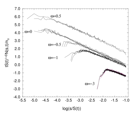
FIG. 12.: Small $x=s/S$ behavior of the scaled mass distributions obtained in numerical simulations for different values of the growth exponent $\omega$.

FIG. 13.: For $\omega=-3$, $S(t)$ grows much faster than $t^{D/(1-\omega)}$ (slope $0.5$) even in the scaling regime ($t>50$) corresponding, a behavior which may be related to logarithmic enhancement of $S$ in mean-field.

V conclusion

In this article, we have extensively studied a generalized Smoluchowski equation corresponding to aggregation processes for which particles (or clusters) grow between collisions, with $\dot{s}=As^{\beta}$, and small particles (monomers) are injected.

A physical motivation for this work is droplets nucleation and we have directly derived generalized Smoluchowski equation and found the collision kernel for two models, respectively describing homogeneous and heterogeneous nucleation.

For a generic kernel, with parameters $\lambda$, $\mu$, we have shown that the gelation criterion was $\max(\lambda,\beta)>1$. We have devoted much time to the study of the equation without injection, for which we have provided two exact solutions. The scaling properties for a generic kernel are seen to be strongly affected by the exogenous growth term, and depend on $\beta$, $\lambda$, and $\mu$. For $\lambda>\beta$, however, the scaling is the same as for the standard equation. For the interesting case $\lambda=\beta$, the behavior of the typical mass $S(t)$ is modified, but the scaling function is unchanged. For $\lambda<\beta$, the scaling function is qualitatively different, and vanishes at a finite $x_{0}>0$.

We have also studied the case of a constant injection rate of monomers. The distribution reaches an asymptotic steady state with a power law tail $N_{\infty}(s)\propto s^{-\tau}$, and we find that $\tau$ depends on $\beta$ and $\lambda$. We have shown that this steady state can be seen as a sol-gel critical state, breaking the mass conservation by collisions, which we think clarifies our physical understanding of these power law asymptotic states.

We have payed special attention to the case of a constant mass injection rate and $\lambda=2\beta-1$, related to homogeneous nucleation. This corresponds to a time-dependent, self-consistent injection rate $I(t)\propto c-M_{\beta}(t)$. We have shown that $I(t)$ vanishes at large time, in agreement with the droplets deposition and coalescence model. For droplets deposition, $M_{\beta}$ is proportional to the surface coverage, and the vanishing of the injection rate corresponds to the saturation of the coverage to $1$. Thus, our self-consistent Smoluchowski’s equation recovers a merely geometrical constraint, which is quite nontrivial.

As far as scaling is concerned, we have found consistent results for $\mu\leq\beta-1$, with nontrivial polydispersity exponents for $\mu=\beta-1$, recovering $\theta=1+\beta$ and $z=1/(1-\beta)$ as for the droplets deposition and coalescence model. However, for $\mu>\beta-1$ kernels, we could not find a consistent scaling, and there might be no scaling solution with a constant mass injection rate. The mean-field kernel for droplets deposition and coalescence has $\mu>\beta-1$, and we argued that taking into account excluded volume pair correlations may be essential to obtain a consistent description by a kinetic equation, including a nontrivial polydispersity exponent if $\mu$ is switched to $\beta-1$. It is quite difficult however to study these correlations either numerically or analytically.

Finally, we have applied these results to droplets growth and coalescence with $d=D$. We have shown that Smoluchowski’s approach accounts for the qualitative difference in the scaling function with the $d<D$ case. We have computed nontrivial polydispersity exponents occurring for $\omega\geq 0$, and described the cross-over from monodispersity to polydispersity occurring for $\omega\to 0^{-}$. We have compared these theoretical results with numerical simulations, with good agreement, despite mean-field limitations which we discussed.

As a conclusion, we would like to point out that one of the main reasons why people have become increasingly interested in breath figures is that it is an example of a geometrically constrained growth process, where diffusion plays a minor role, in contrast with diffusion limited cluster-cluster aggregation [meakin83, kolb83, meakinrev92] or Brownian coalescence of droplets [meakindyn90]. Therefore, one could doubt that neglecting density-density correlations may have no dramatic consequences. Indeed, for homogeneous nucleation, we have seen that pair correlations may be crucial to find a correct scaling function, and we also found an infinite upper critical dimension for heterogeneous $d=D$ nucleation. However, we have shown that Smoluchowski’s equation in an extended form could be successfully used to describe heterogeneous growth, and also gives very interesting insights into homogeneous growth, which was not a priori obvious.

We are very grateful to P.L. Krapivsky for helpful correspondence.

A Scaling theory without injection

In this appendix, we shall give a detailed demonstration of the scaling results given in Sec. III B 2 for generalized Smoluchowski’s equation without injection of monomers. We make the assumption that starting from a monodispersed distribution of droplets, the late time solution of Eq. (31) has the scaling form of Eq. (50). Note that, although it is quite clear from its homogeneity behavior that Smoluchowski’s equation admits scaling solutions, it has never been mathematically proved that these solutions are approached at large times, except in the few cases for which we can obtain the exact solution. However, scaling is commonly observed experimentally and numerically for aggregation models, as well as in numerical solutions of Smoluchowski’s equation [krivitsky95] (when possible), making this assumption very reasonable.

Another important remark is that Smoluchowski’s equation may generally speaking admit different classes of scaling solutions, with different asymptotic behavior, and that one peculiar class will be selected from the initial condition. This must be remembered in the discussion. In our demonstration, we shall always use the fact that $S(t)$ cannot be negligible compared to $s_{0}(t)\sim t^{1/{(1-\beta)}}$, the lower cut-off, from the discussion in Sec. III B 2. We shall also implicitly assume that $Y(t)$, $S(t)$ and all the moments of $N(s,t)$ are asymptotically regular convex or concave functions.

1 Within the nongelling domain

To start with, let us study the case $\lambda<1$ and $\beta<1$, i.e. nongelling systems which are not on the gelling boundary. Our discussion is based on the fact that either $S(t)\gg s_{0}(t)$ or $S(t)\propto s_{0}(t)$. We shall study the implications of both possibilities.

a Case $S\gg s_{0}$

Let us assume that $S(t)\gg s_{0}(t)$, or equivalently that $S^{\beta-1}\ll\dot{S}/{S}$. We see that the growth term (58) is much smaller than (57) in the scaling limit, and the scaling equation is,

$$bxf^{\prime}(x)+af(x)=f(x)\int_{0}^{+\infty}f(x_{1})K(x,x_{1})dx_{1}$$ (A1)

$$-\frac{1}{2}\int_{0}^{x}f(x_{1})f(x-x_{1})K(x_{1},x-x_{1})\,dx_{1}$$ (A2)

where $b=\lim\,\dot{S}S^{-2-\lambda}Y$ and $a=\lim\,\dot{Y}S^{-1-\lambda}$ are positive, and possibly zero or infinite.

For finite $a$ and $b$, this equation is very close from standard Smoluchowski equation Eq. (1) with the same kernel $K$, which corresponds to $a=2b$ and $0<a<+\infty$ and was well studied in the literature [vdg85prl, vdg87scal, nontriv97]. The polydispersity exponent $\tau$, if any, has the upper bound $\tau\leq 1+\lambda<2$ (read Sec. III B 3). As a consequence, from Eq. (54) we have,

$$M_{1}(t)\propto S^{2}/Y$$ (A3)

From Eq. (60), we see that $M_{1}(t)$ is nondecreasing. Thus, either $M_{1}(t)$ tends to a finite limit, or it goes to infinity.

(i) If $M_{1}(t)$ tends to a finite limit, then, necessarily from Eq. (A3), $Y\propto S^{2}$. The scaling of (57) with (59) requires $\dot{S}\propto S^{\lambda}$, hence,

$$S(t)\propto t^{\frac{1}{1-\lambda}}$$ (A4)

To be consistent with our assumption that $S(t)\gg t^{1/(1-\beta)}$, we must have $\lambda>\beta$. Besides, from Eq. (60), a necessary condition for $M_{1}(t)$ to have a large $t$ finite limit is that $M_{\beta}(t)$ must be an integrable function. If $\tau<1+\beta$, $M_{\beta}$ scales as $S^{1+\beta}/Y$, i.e. $M_{\beta}\propto t^{(\beta-1)/(1-\lambda)}$ and is integrable since $\lambda>\beta$.

If $\tau>1+\beta$, we have, from Eq. (55),

$$M_{\beta}\propto S(t)^{\tau-2}s_{0}(t)^{1+\beta-\tau}\ll s_{0}(t)^{\beta-1}\propto t^{-1}$$ (A5)

since $\tau<2$ and $S(t)\gg s_{0}(t)$. Therefore, $M_{\beta}$, being equivalent to a power law $\ll 1/t$, is integrable.

If $\tau=1+\beta$, from Eq. (56),

$$M_{\beta}\propto S(t)^{\beta-1}\ln(S/s_{0})\propto t^{\frac{\beta-1}{1-\lambda}}\ln t$$ (A6)

which is integrable when $\lambda>\beta$.

(ii) Now, let us consider the case when $M_{1}(t)$ diverges at large time. From Eqs. (60), (A3), (55) and (56), we obtain,

$$\dot{M_{1}}\propto\left\{\begin{array}[]{lr}M_{1}S^{\beta-1},&\qquad\mbox{if }\tau<1+\beta\\ M_{1}S^{\tau-2}s_{0}(t)^{1+\beta-\tau},&\qquad\mbox{if }\tau>1+\beta\\ M_{1}S^{\beta-1}\ln(S/s_{0}),&\qquad\mbox{if }\tau=1+\beta\end{array}\right.$$ (A7)

Anyway, in the three cases, $S\gg s_{0}$ implies that $\dot{M_{1}}\ll M_{1}s_{0}^{\beta-1}$, hence,

$$\dot{M_{1}}\ll\frac{M_{1}}{t}$$ (A8)

Therefore $M_{1}(t)\ll t^{\alpha}$ for any $\alpha>0$. From Eq. (A3) and the fact that $\dot{S}/{S}$ is at least of order $1/t$ since $S(t)\gg t^{1/(1-\beta)}$, Eq. (A8) requires that,

$$2\frac{\dot{S}}{S}\sim\frac{\dot{Y}}{Y}$$ (A9)

Thus, the scaling condition between (57) and (59) is simply,

$$\frac{\dot{S}}{S}\propto\frac{S^{1+\lambda}}{Y}\propto M_{1}S^{\lambda-1}$$ (A10)

which implies that $S^{1-\lambda}$ is dominated by a power law. Combined with the fact that $S(t)\gg t^{1/(1-\beta)}$, this requires that

$$\frac{\dot{S}}{S}\propto\frac{1}{t}$$ (A11)

and

$$M_{1}\propto t^{-1}S^{1-\lambda}\gg t^{\frac{\beta-\lambda}{1-\beta}}$$ (A12)

thus, from Eq. (A8), we must have $\lambda\geq\beta$. Now, combining Eqs. (A12) and (A7), we see that,

$$\dot{M_{1}}\propto M_{1}^{-\alpha_{1}}t^{-\alpha_{2}}(\ln(t^{\frac{\lambda-\beta}{1-\beta}}M_{1}))^{\alpha_{3}}$$ (A13)

($\alpha_{3}=1$ if $\tau=1+\beta$, otherwise $\alpha_{3}=0$).

Since $M_{1}\to\infty$, the right hand side of the latter equation must be non integrable, and as $M_{1}$ is much smaller than any positive power of $t$, this implies that $\alpha_{2}\leq 1$.

$$\alpha_{2}=\left\{\begin{array}[]{ll}\frac{1-\beta}{1-\lambda},&\qquad\mbox{if }\lambda\leq\beta\\ \frac{2-\tau}{1-\lambda}+\frac{\tau-1-\beta}{1-\beta},&\qquad\mbox{if }\tau>1+\beta\end{array}\right..$$ (A14)

Since $\tau\leq 1+\lambda$, $\alpha_{2}>1$ if $\lambda>\beta$. Therefore we must have $\lambda\leq\beta$. However we already found that $\lambda\geq\beta$, thus $\lambda$ must be equal to $\beta$.

As a consequence $\tau$ is never bigger than $1+\beta=1+\lambda$. and we can distinguish between $\mu>0$ kernels, for which $\tau=1+\lambda=1+\beta$ and $\mu\leq 0$ kernels for which there is no polydispersity exponent or $\tau<1+\beta$.

Let us start with $\mu\leq 0$ kernels. As $\tau<1+\beta$, and $\lambda=\beta$, Eq. (A13) is reduced to $\dot{M_{1}}\propto 1/t$, which leads to,

$$M_{1}(t)\propto\ln t.$$ (A15)

For a $\mu>0$ kernel, $\tau=1+\lambda=1+\beta$, and Eq. (A13) leads to,

$$\dot{M_{1}}\propto(\ln M_{1})/t,$$ (A16)

and it is easily seen that,

$$M_{1}(t)\propto(\ln t)\ln(\ln t).$$ (A17)

In both cases, we have,

$$S(t) \propto (tM_{1})^{\frac{1}{1-\beta}},$$ (A18)

$$Y(t) \propto S^{2}/M_{1}.$$ (A19)

Thus, the initial assumption that $S(t)\gg s_{0}(t)$ implies that $\lambda\geq\beta$ and that the scaling equation is Eq. (A1) with $a=2b$ (since $2\dot{S}/{S}\sim\dot{Y}/{Y}$) and $0<a<+\infty$, and is the same as for standard Smoluchowski’s equation with the same kernel.

b Case $S\propto s_{0}$

Conversely, let us assume that $S(t)\propto t^{1/(1-\beta)}$. If $\dot{Y}/{Y}\gg\dot{S}/{S}\propto 1/t$, $Y$ increases faster than any power law, the growth term is still negligible at large time, and Eqs. (57) and (59) are of the same order, hence $S^{1+\lambda}/Y\propto\dot{Y}/{Y}$, which is contradictory, for $S^{1+\lambda}/Y$ vanishes faster than any power law while $\dot{Y}/{Y}\gg 1/t$.

Thus, $\dot{Y}/{Y}=O(\dot{S}/{S})$ and both terms in the right hand side of Smoluchowski’s equation are of the same order at large time, as $\dot{S}/{S}\propto S^{\beta-1}$. Besides, both terms must scale as the collision term, otherwise the obtained scaling equation has no physical solution vanishing below a finite argument $x_{0}>0$. Thus, (58) and (59) must be of the same order, which yields:

$$\frac{S^{\beta-1}}{Y}\propto\frac{S^{1+\lambda}}{Y^{2}}.$$ (A20)

and $Y(t)\propto S(t)^{2+\lambda-\beta}$. The fact that the scaling function vanishes at a finite $x_{0}>0$ ensures that, $M_{1}(t)\propto S^{2}/Y$, hence,

$$M_{1}(t)\propto S(t)^{\beta-\lambda}.$$ (A21)

Since $M_{1}(t)$ is non decreasing, we must have $\lambda\leq\beta$. However, if $\lambda=\beta$, Eq. (35) yields

$$\dot{M_{1}}\propto 1/t,$$ (A22)

hence $M_{1}(t)\propto\ln t$, which is in contradiction with Eq. (A21). Therefore one must have $\lambda<\beta$.

The scaling equation has the form,

$$b\left[\theta f(x)+xf^{\prime}(x)\right]-a(x^{\beta}f(x))^{\prime} = f(x)\int_{0}^{+\infty}f(x_{1})K(x,x_{1})dx_{1}$$ (A24)

$$-\frac{1}{2}\int_{0}^{x}f(x_{1})f(x-x_{1})K(x_{1},x-x_{1})\,dx_{1}$$

c Conclusion

Since $S(t)\geq s_{0}(t)$, the collection of the two cases we examined above leads to the conclusion that, if $\lambda<1$ and $\beta<1$, there are three main regimes of scaling, in agreement with the qualitative discussion in Sec III B 2.

If $\beta>\lambda$, $S(t)$ scales as $S_{g}(t)\propto t^{1/(1-\beta)}$, $Y(t)\propto S(t)^{\theta}$, with $\theta=2+\lambda-\beta$, and there is no polydispersity exponent since the scaling function is zero below a finite $x_{0}$.

If $\beta<\lambda$, $S(t)$ scales as $S_{c}(t)\propto t^{1/(1-\lambda)}$, the mass is asymptotically conserved, i.e. $M_{1}(t)$ tends to a constant, and $\theta=2$. There can be a polydispersity exponent, which is the same as for standard Smoluchowski’s equation Eq. (1) with the same kernel.

Eventually, in the marginal case when $\lambda=\beta$, the scaling of $S(t)$ depends on the kernel not only through its homogeneity $\lambda$, but also through its $\mu$ exponent. As in the $\beta<\lambda$ case, the scaling equation is the same as for Smoluchowski’s equation with the same kernel. For $\mu\leq 0$ kernels, the mass in the system $M_{1}(t)\propto\ln t$, while for $\mu>0$ kernels, with $\tau=1+\lambda$, $M_{1}(t)\propto t(\ln t)\ln(\ln t)$. In both cases, $S\propto(tM_{1})^{1/(1-\beta)}$ and $Y\propto S^{2}/M_{1}$.

These scaling results can be compared to the case $K=1$,$\beta=0$ which we solved exactly: we found that the conventional scaling breaks down and that, with the proper scaling form, the scaling function is the same as for the exactly solvable standard Smoluchowski’s equation without the growth term, that $S(t)\propto(t\ln t)$, $M_{1}(t)\propto\ln t$ and $Y\propto t^{2}\ln t$, just as predicted by the scaling theory.

2 $\lambda=1$ and $\beta<1$

For $\lambda=1$ and $\beta<1$, it is possible to follow the same line of reasoning, with a few modifications. In this case, one has to distinguish between $\mu>0$ and $\mu\geq 0$ (this is also true for standard Smoluchowski’s equation with $\lambda=1$ [vdg87scal]), since for $\mu>0$, we find $\tau=2$ and the scaling of $M_{1}$ has an extra $\ln(S/s_{0})$. It is found that $M_{1}$ is asymptotically conserved, that $S(t)\gg s_{0}(t)$, and that the scaling equation is Eq. (A1) with $a=2b<+\infty$. For $\mu>0$, one has $\dot{S}\propto S/(\ln S)$, which leads to,

$$S(t)\propto e^{b\sqrt{t}},$$ (A25)

whereas if $\mu\leq 0$,

$$S(t)\propto e^{bt},$$ (A26)

where $b$ cannot be derived from the scaling theory.

3 $\beta=1$ and $\lambda<1$

In this case $s_{0}(t)\propto e^{t}$, and the discussion is quite different. From Eq. (60), we see that:

$$M_{1}(t)=M_{1}(0)\,e^{t}.$$ (A27)

Since $S(t)\geq s_{0}(t)\propto e^{t}$, we have in the large time limit $\dot{S}/S\geq 1$. Let us assume that $\dot{S}/{S}\gg 1$, i.e. that $S(t)$ is bigger than any exponential function $e^{\alpha t}$, which entails that (57) is much bigger than (58) (which scales as $1/Y$ since $\beta=1$). From Eqs. (54), (55) and (56), it is clear that,

$$S^{2}/Y=O(M_{1}(t))=O(e^{t}).$$ (A28)

Consequently, if (57) scales as (59), then $\dot{S}/{S^{\lambda}}=O(e^{t})$ and $\dot{Y}/{Y^{(1+\lambda)/2}}=O(e^{t/2})$. Since $\lambda<1$, these two relations are in contradiction with the assumption that $S$ is much bigger than any exponential function (which implies the same property for $Y$, through Eq. (A28)). We see that if $\dot{S}/{S}\gg 1$ , (57) is the leading term in the scaling limit, and the scaling function is a pure power law $f(x)=cx^{-\tau}$ with $\tau=\lim(\dot{Y}/Y)(S/\dot{S})$. One must have $\tau>2$ such that the total mass in the system be finite at finite time in the scaling regime. Making use of Eq. (55), we find that $n(t)\propto M_{1}(t)/s_{0}(t)$ would tend to a finite value $n_{\infty}>0$, which is unphysical.

Therefore $\dot{S}/{S}$ is of order $1$. From arguments very similar to those we just used, it is easily seen that $\dot{Y}/{Y}$ cannot be much bigger than $1$. Thus, (57) scales as (58). If $\dot{Y}/Y\to 1$ and $\dot{S}/S\to 1$, the left hand side of Eq. (31) vanishes and we have to take into account the subleading terms in the scaling limit. This occurs for $\lambda=0$ as will be seen below.

If the left hand side does not vanish, the scaling with (59) leads to $S^{1+\lambda}\propto Y$, and the scaling equation is once again Eq. (A1), but now with $b/a=(1-\dot{S}/{S})/(1-\dot{Y}/{Y})$. Consequently, the polydispersity exponent, if any, is less than $1+\lambda$, and Eq. (A3) holds, leading to $S^{2}\propto Y\,e^{t}$. Since $S^{1+\lambda}\propto Y$, we have,

$$S(t) \propto e^{\frac{t}{1-\lambda}}$$ (A29)

$$Y(t) \propto S^{2}\,e^{-t}$$ (A30)

which excludes $\lambda<0$ since $S(t)\geq s_{0}(t)=e^{t}$, and also $\lambda=0$ for which $\dot{S}/S\to 1$ and $\dot{Y}/Y\to 1$. Note that in the $\lambda>0$ case, we find $a=2b$, and once again the scaling equation is the same as for standard Smoluchowski’s equation.

Indeed, for the exactly solvable case $K=1,\,\beta=1$, which corresponds to $\lambda=0$, we found that $S(t)\propto te^{t}$ and $Y(t)\propto S^{2}/e^{t}$, thus $\dot{S}/S\to 1$ and $\dot{Y}/Y\to 1$. Thus, to treat the $\lambda=0$ case, we shall write $S(t)=X(t)M_{1}(t)$, with $\dot{X}/X\ll 1$, and we have $Y\propto S^{2}/M_{1}=XS$. The right hand side of Eq. (31) scales as,

$$-\frac{1}{Y}(2f(x)+xf^{\prime}(x))\frac{\dot{X}}{X},$$ (A31)

while the left hand side scales as

$$\frac{S}{Y^{2}}(..)\propto\frac{X}{Y}(..)$$ (A32)

which leads to $X(t)\propto t$, recovering the exact result for $K=1$. Once again the scaling function is Eq. (A1) with $a=2b<+\infty$. The polydispersity exponent $\tau$ is strictly less than $2$, which justifies a posteriori that $Y\propto S^{2}/M_{1}$ (it is possible to show that assuming $\tau>2$ leads to a contradiction).

However, for $\lambda<0$, we were unable to find a consistent scaling.

4 $\lambda=1$ and $\beta=1$

In this case, we still have $M_{1}(t)\propto e^{t}$ and $s_{0}(t)\sim e^{t}$, but it is easily seen with the same kind of arguments as above, that one must have $\dot{S}/{S}\gg 1$. Thus the exogenous growth term (58) is negligible, and the scaling of (57) and (58) yields, $\dot{S}/S\propto S^{2}/Y$.

For $\mu\leq 0$ kernels, one has $M_{1}\propto S^{2}/Y$ and we obtain $\dot{S}/S\propto e^{t}$, leading to,

$$S(t)\propto e^{be^{t}}.$$ (A33)

For $\mu>0$, we have $\tau=2$ and $M_{1}\propto S^{2}\ln(S/e^{t})/Y$, leading to $\dot{S}/S\propto e^{t}/\ln(S)$, and,

$$S(t)\propto e^{b\sqrt{e^{t}}}.$$ (A34)

In these expressions $b$ is an unknown positive constant.