Charge correlations and optical conductivity in weakly doped antiferromagnets

Abstract

We investigate the dynamical charge-charge correlation function and the optical conductivity in weakly doped antiferromagnets using Mori-Zwanzig projection technique. The system is described by the two-dimensional $t$-$J$ model. The arising matrix elements are evaluated within a cumulant formalism which was recently applied to investigate magnetic properties of weakly doped antiferromagnets. Within the present approach the ground state consists of non-interacting hole quasiparticles. Our spectra agree well with numerical results calculated via exact diagonalization techniques. The method we employ enables us to explain the features present in the correlation functions. We conclude that the charge dynamics at weak doping is governed by transitions between excited states of spin-bag quasiparticles.

The dynamical properties of the normal state of the superconducting cuprates are still not completely understood. A much discussed question about strongly correlated electronic systems in two dimensions is whether they can be described as Fermi liquids or not. In Fermi liquids the low-lying spin and density excitations can be considered as particle-hole excitations of fermionic quasiparticles. In contrast, one-dimensional correlated systems show spin-charge separation, i.e. spin and charge excitations are different elementary excitations, and the ”physical” electron can be interpreted as a composite object.

Theoretical progress in this field is mostly based on numerical techniques, especially on exact diagonalization methods [1, 2, 3] and Lanczos calculations [4]). However, the system sizes presently accessible leave many problems unresolved. Meanwhile, the spin response of doped antiferromagnets has been studied in a number of analytical papers but only few authors have investigated the charge density response function [5, 6].

In this paper we present analytical results based on projection technique calculations for dynamical charge-charge correlation functions in weakly doped 2D antiferromagnets. The system is described by the 2D $t$-$J$ model:

$$H\,=\,-t\sum_{\langle ij\rangle\sigma}(\hat{c}^{\dagger}_{i\sigma}\hat{c}_{j\sigma}+\hat{c}^{\dagger}_{j\sigma}\hat{c}_{i\sigma})+J\sum_{\langle ij\rangle}\ ({\bf S}_{i}{\bf S}_{j}-{{n_{i}n_{j}}\over 4})\,.$$ (1)

The symbol $\langle ij\rangle$ refers to a summation over pairs of nearest neighbors. The two antiferromagnetic sublattices will be denoted by $\uparrow$ and $\downarrow$. The electronic creation operators $\hat{c}_{i\sigma}^{\dagger}$ exclude double occupancies.

We study the Laplace transform of the time- and wave-vector dependent charge-charge correlation function at zero temperature defined by

$$G_{\rho}({\bf k},z)\,=\,\langle\psi_{0}|\,\rho_{\bf k}^{\dagger}{1\over{z-L}}\rho_{\bf k}^{\phantom{\dagger}}\,|\psi_{0}\rangle$$ (2)

Here, $\rho_{\bf k}=\sum_{{\bf q},\sigma}c_{{\bf k+q},\sigma}^{\dagger}c_{{\bf q}\sigma}^{\phantom{\dagger}}=\sum_{i\sigma}{\rm e}^{{\rm i}{\bf k}{\bf R}_{i}}c_{i\sigma}^{\dagger}c_{i\sigma}^{\phantom{\dagger}}$ is the Fourier-transformed charge density operator. $|\psi_{0}\rangle$ denotes the exact ground state of the system, $z=\omega+{\rm i}\eta$ is the complex frequency variable. The Liouville operator $L$ is a superoperator defined by $LA=[H,A]_{-}$ for any operator $A$. At zero temperature the optical conductivity $\sigma(\omega)$ for frequencies $\omega>0$ is related to the charge response function $G_{\rho}({\bf k},\omega)$ as follows:

$${\rm Re}\,\sigma(\omega)\,=\,{{\rm e}^{2}\over cN}\lim_{{\bf k}\rightarrow 0}\frac{\omega\,{\rm Im}\,G_{\rho}({\bf k},\omega)}{{\bf k}^{2}}\,$$ (3)

where $N$ is the total particle number. Eq. (3) follows from the continuity relation $L\rho_{\bf k}={\bf k}\cdot{\bf j}_{\bf k}$ where ${\bf j}_{\bf k}$ is the charge current operator.

In the following, we apply a projection technique [7] approach to determine the charge-density response function. The arising matrix elements are evaluated using a cumulant formalism [8, 9] which has been recently introduced to investigate ground-state properties of correlated electronic systems. We are interested in calculating dynamical correlation functions for a set of operators $B_{\nu}$

$$G_{\nu\mu}(z)\,=\,\langle\psi_{0}|\,\delta B_{\nu}^{\dagger}{1\over{z-L}}\delta B_{\mu}^{\phantom{\dagger}}\,|\psi_{0}\rangle$$ (4)

with $\delta B_{\nu}=B_{\nu}-\langle\psi_{0}|B_{\nu}|\psi_{0}\rangle$. Using cumulants these correlation functions can be rewritten as [9]

$$G_{\nu\mu}(z)\,=\,\langle\phi_{0}|\,\Omega^{\dagger}\,B_{\nu}^{\dagger}\left({1\over{z-L}}B_{\mu}^{\phantom{\dagger}}\right)^{\cdot}\,\Omega\,|\phi_{0}\rangle^{c}$$ (5)

The operator $\Omega$ has similarity to the so-called wave operator (or Moeller operator known from scattering theory). Within cumulants it transforms the ground state $|\phi_{0}\rangle$ of the unperturbed system $H_{0}$ into the exact ground state $|\psi_{0}\rangle$ of $H=H_{0}+H_{1}$. Explicitly it is given by [8]

$$\Omega=1+\lim_{x\to 0}{1\over{x-(L_{0}+H_{1})}}H_{1}\,.$$ (6)

The brackets $\langle\phi_{0}|\,...\,|\phi_{0}\rangle^{c}$ denote cumulant expectation values with $|\phi_{0}\rangle$. The dot $\cdot$ in Eq. (5) indicates that the quantity inside $(...)^{\cdot}$ has to be treated as a single entity in the cumulant formation. $L_{0}$ is the Liouville operator corresponding to $H_{0}$, i.e., $L_{0}A=[H_{0},A]_{-}$. The relation (5) can be applied to either weakly or strongly correlated systems because its use is independent of the operator statistics , i.e., it is valid for fermions, bosons or spins.

Using Mori-Zwanzig projection technique [7] one can derive a set of equations of motion for the dynamical correlation functions $G_{\nu\mu}(z)$. Neglecting the self-energy terms as explained below it reads:

$$\sum_{\nu}\left(z\delta_{\eta\nu}-\omega_{\eta\nu}\right)\,G_{\nu\mu}(z)\,\,=\,\,\chi_{\eta\mu}\,.$$ (7)

$\chi_{\eta\nu}$ and $\omega_{\eta\nu}$ are the static correlation functions and frequency terms, respectively. They are given by the following cumulant expressions:

$$\chi_{\eta\nu}\, = \,\,\langle\phi_{0}|\,\Omega^{\dagger}\,B_{\eta}^{\dagger}B_{\nu}^{\phantom{\dagger}}\,\Omega\,|\phi_{0}\rangle^{c}\,,$$ (8)

$$\omega_{\eta\nu}\, = \,\,\sum_{\lambda}\langle\phi_{0}|\,\Omega^{\dagger}\,B_{\eta}^{\dagger}(LB_{\lambda}^{\phantom{\dagger}})^{\cdot}\,\Omega\,|\phi_{0}\rangle^{c}\,\chi_{\lambda\nu}^{-1}\,,$$ (9)

$\chi_{\nu\mu}^{-1}$ is the inverse matrix of $\chi_{\nu\mu}$. These terms describe all dynamic processes within the subspace of the Liuoville space spanned by the operators $B_{\nu}$.

Next we outline the description of the ground state of the $t$-$J$ model at weak doping within the cumulant formalism, details have been published recently [10]. $\delta$ denotes the hole concentration away from half filling, i.e., the system with $N$ lattice sites possesses $M=\delta N$ dopant holes. The Hamiltonian is decomposed into $H_{0}$ and $H_{1}$ as follows:

$$H_{0}\,=\,H_{Ising}\,,\quad H_{1}\,=\,H_{t}\,+\,H_{\bot}\,.$$ (10)

The ground state $|\phi_{0}\rangle$ of the unperturbed Hamiltonian $H_{0}$ is an antiferromagnetically ordered Néel state with $M$ holes. The holes have fixed momenta ${\bf k}_{m}$ and are located on the sublattice $\sigma_{m}$ ($\sigma_{m}=\uparrow,\downarrow$)

$$|\phi_{0}\rangle\,\, = \,\,\hat{c}_{{\bf k}_{1}\sigma_{1}}\,\ldots\,\hat{c}_{{\bf k}_{M}\sigma_{M}}\,|\phi_{N{\mathaccent 19{e}}el}\rangle\,,$$ (11)

$$\hat{c}_{{\bf k}\uparrow}\,\, = \,\,(N/2)^{-1/2}\sum_{i\in\uparrow}\,{\rm e}^{i\,{\bf k}{\bf R}_{i}}\,\hat{c}_{i\uparrow}\,,\quad\hat{c}_{{\bf k}\downarrow}\,\,=\,\,(N/2)^{-1/2}\sum_{i\in\downarrow}\,{\rm e}^{i\,{\bf k}{\bf R}_{i}}\,\hat{c}_{i\downarrow}\,.$$ (12)

Within the cumulant method we employ an exponential ansatz [11] for the wave operator $\Omega$, i.e., $\Omega={\rm e}^{S}$. The operator $S$ describes the effect of the perturbation $H_{1}$ onto the unperturbed ground state $|\phi_{0}\rangle$. We are basically interested in the charge dynamics of the system. Therefore we assume that background spin fluctuations can be neglected. To treat hole motion processes induced by $H_{t}$ the concept of path operators [12] is used which leads to the picture of spin-bag quasiparticles [13]. Here we define path concatenation operators $A_{n,\rho}(i)$ where $i$ denotes a lattice site, $n$ the path length, and $\rho$ the individual path shape: $A_{n,\rho}(i)$ operating on a hole at site $i$ in the state (12) moves the hole $n$ steps away and creates a path or string of $n$ spin defects attached to the transferred hole. Note that there is a number $m_{n}$ of different path shapes for a given path length n. For $n=1$ there are $m_{1}=4$ different paths, for $n=2$ $m_{2}=12$ and so on. Having defined the excitation operators $A_{n,\rho}(i)$, the wave operator $\Omega$ of the cumulant formalism takes the form

$$\Omega\,=\,{\rm exp}\left(\,\sum_{n=1}^{n_{max}}\sum_{\rho=1}^{m_{n}}\lambda_{n,\rho}A_{n,\rho}\,\right)\,,\quad A_{n,\rho}\,=\,\sum_{i}A_{n,\rho}(i)$$ (13)

with parameters $\lambda_{n,\rho}$ yet unknown. Note the additional definiton $A_{0}(i)={1\over 2}\sum_{\sigma}\hat{c}_{i\sigma}^{\phantom{\dagger}}\hat{c}_{i\sigma}^{\dagger}$ which is the only ”path” with zero length ($\rho=1$). The path operators $A_{n,\rho}$ commute with each other because they only contain spin-flip operators destroying Néel order.

Following ref. [11] one attains a non-linear set of equations for the ground-state energy $E_{0}$ and the coefficients $\lambda_{n,\rho}$:

$$E_{0}\,=\,\langle\phi_{0}|H\Omega|\phi_{0}\rangle^{c}\,,\quad 0\,=\,\langle\phi_{0}|A_{n,\rho}^{\dagger}\,H\,\Omega\,|\phi_{0}\rangle^{c}$$ (14)

with $\Omega$ given by (13). The cumulant expectation values have to be taken with respect to the unperturbed ground state (12). The set of equations (14) together with the additional approximation of independent hole quasiparticles leads to a generalized eigenvalue problem. For details see [10]. The used picture of independent quasiparticles is appropriate for small hole concentrations, i.e., for a dilute gas of holes moving in an antiferromagnetic background.

For the application of Mori-Zwanzig projection technique one has to choose a set of relevant operators $B_{\nu}$. Here we are going to neglect the self-energy terms obtained within projection technique, cf. (7). Therefore we need to use a sufficiently large set of operators $B_{\nu}$ to cover the charge dynamics. One variable to include is the charge density operator $\rho_{\bf k}$ itself. The other variables should provide a coupling between the ground state $\Omega|\phi_{0}\rangle$ and all excited states of $H$. These variables are obtained by applying the perturbation $H_{1}$ to $\rho_{\bf k}$. Assuming that the charge dynamics is mainly carried by spin-bag quasiparticles we can define

$$B_{n,\rho}({\bf k})\,\,=\,\,\sum_{i}e^{{\rm i}{\bf k}{\bf R}_{i}}\,\,A_{n,\rho}(i)\,A_{0}(i)^{\dagger}\,\,=\,\,\sum_{i}e^{{\rm i}{\bf k}{\bf R}_{i}}\,\,B_{n,\rho}(i)\,.$$ (15)

As explained above, $A_{n,\rho}(i)$ is a path operator of length $n$ with the path shape $\rho$ acting on a hole at site $i$. The indices $n,\rho$ replace the general index $\nu$ of the dynamical variables $B_{\nu}$ in Eqs. (4,5). The Fourier-transformed operator $B_{n,\rho}(i)$ couples to a hole (at site $i$) and adds the path $A_{n,\rho}$. So the relevant part of the Liouville space spanned by the operators $B_{n,\rho}$ contains all individual path states connected to the holes.

The first of these operators is the hole density operator itself:

$$B_{0,1}({\bf k})\,=\,{1\over 2}\rho_{\bf k}^{hole}\,=\,{1\over 2}\sum_{i\sigma}{\rm e}^{{\rm i}{\bf k}{\bf R}_{i}}\,\,{\hat{c}}_{i\sigma}^{\phantom{+}}{\hat{c}}_{i\sigma}^{\dagger}$$ (16)

The quantity we are interested in is therefore the diagonal correlation function $G_{\nu\nu}({\bf k},z)$ with $\nu=(0,1)$. Note that particle density and hole density are equivalent quantities.

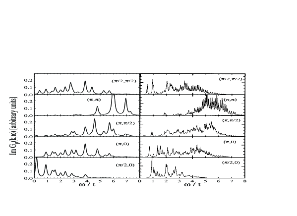
FIG. 1.: Left panel: charge-charge correlation function obtained from the present calculation for $t/J$ = 2.5, very small $\delta$, $n_{max}=5$, and different momentum transfers, plotted with Lorentzians using an artificial linewidth of 0.1 $t$. Right panel: Exact diagonalization data from [1] for comparison, $t/J=2.5$ (see also [5]). The numerical data have been calculated for a 4 x 4 periodic cluster and a hole concentration of $\delta=25\%$.

Our results for the charge-response function ${\rm Im}\,G_{\rho}({\bf k},\omega)$ at $t/J=2.5$ are shown in Fig. 1. The intensity of the spectra is proportional to the hole concentration $\delta$. For small momentum the spectral weight is mainly concentrated in a peak near $\omega=0$ (with an energy scaling with ${\bf v}_{F}\cdot{\bf k}$ for ${\bf k}\rightarrow 0$). With increasing momentum we find a transfer of spectral weight to higher energies. Calculations for other values of $t/J$ show that the broad structures observed in the spectra for large momenta scale with $t$, e.g., the maximum spectral weight in the charge-response function at $(\pi,\pi)$ remains at energies of about $6t$. The right panel of Fig. 1. shows exact diagonalization data for $\delta=25\%$ taken from ref. [1]. We observe a good agreement of the spectra, some differences may be either due to the small number of sites in the numerical calculations (which leads to an energy gap in all spectra and other finite-size effects) or due to the neglection of relaxation processes in the present calculation (such processes would produce finite linewidths).

For the interpretation of the calculated spectra one can consider the one-hole spectrum of the Hamiltonian within our approximation. From the diagonalization of the one-hole problem in the subspace of path operators $A_{n\rho}$ one obtains several bands for the spin-bag quasiparticles. As is well known, the lowest band has a minimum at $(\pm\pi/2,\pm\pi/2)$ and a bandwidth of about $2J$. It corresponds to a quasiparticle with s-like symmetry. The spin-bag states in the higher bands have nodes in the coefficients $\lambda_{n,\rho}$. The low-energy peak in the spectra (visible at momentum transfer $(\pi/2,0)$ ) corresponds to excitations within the lowest quasiparticle band whereas the high-energy part arises from transitions to higher bands.

FIG. 2.: Optical conductivity for small hole concentration and different $t/J$. The spectra have been calculated from the charge-charge correlation function using (3).

Using Eq. (3) one can deduce the optical conductivity from the calculated charge response function. Results for ${\rm Re}\,\sigma(\omega)$ are displayed in Fig. 2. They show again good agreement with the numerical results from ref. [3] for $\delta=12.5\%$. The main peak (at low energy) scales with $J$, it is located at $\approx 1.7J$. It arises from the transition between the first and second quasiparticle band, i.e., from the s-like groundstate to a p-like state. So our calculation supports the discussion given in ref. [3] where only these two states have been considered in a simplified analytical calculation for the main peak. We want to emphasize that taking into account all string states (up to a truncation length) as done in the present work reproduces not only this main peak but also the incoherent continuum found at energies up to $6t$. The low-energy peak corresponding to $\omega\approx$ 0.3 eV for $J=$ 0.15-0.2 eV which was also found in numerical studies of the $t$-$J$ and Hubbard models is supposed to coincide with the mid-infrared peak observed in optical spectra of high-$T_{c}$ superconductors (see e.g. [14]). Within the present calculation we do not obtain a Drude peak $D\,\delta(\omega)$ since Eq. (3) is valid for non-zero frequency only, i.e., it does not include the diamagnetic part of the current. The different scaling behaviour of $G_{\rho}(\bf k,\omega)$ (for large $\bf k$) and $\sigma(\omega)$ with $t/J$ arises from the internal structure of the spin bag forming the quasiparticle. Details will be published elsewhere [15].

The agreement of our data with the exact diagonalization results [1, 3] is remarkable because these numerical calculations are done for rather large hole concentrations (e.g., 25%) where only short-range magnetic order is present in the high-$T_{c}$ materials. In contrast, the present calculations are based on magnetic long-range order. Thus we conclude that whether the quasiparticles move in a long-range ordered background or not does not have an essential influence on the charge response of the system. The dynamics is mainly determined by the local antiferromagnetic order in the vicinity of the hole quasiparticles [16], i.e., the magnetic correlation length has to be of the order of the quasiparticle size.

One should note that a recent slave-boson approach [5] to the charge dynamics in the $t$-$J$ model also reproduces some key features of the charge response function, namely a peak at small energy for small ${\bf k}$ and a broad featureless continuum at energies of several $t$. The theory presented there is based on a Fermi liquid picture and completely neglects antiferromagnetic correlations in the ground state. However, in the high-$T_{c}$ materials short-range correlations are present also at higher hole concentrations. We believe them to be important for the structure of the spectra.

Summarizing, we conclude that the charge dynamics in the weakly doped $t$-$J$ model can be well explained within the picture of independent spin-bag quasiparticles and their excitations. The present calculation may serve as a basis for the investigation of the charge dynamics in more realistic models for the cuprate superconductors, as e.g. the three-band Hubbard model.

REFERENCES

- [1] T. Tohyama, P. Horsch, and S. Maekawa, Phys. Rev. Lett. 74, 980 (1995).
- [2] R. Eder, Y. Ohta, and S. Maekawa, Phys. Rev. Lett. 74, 5124 (1995).
- [3] R. Eder, P. Wrobel, and Y. Ohta, Phys. Rev. B 54, R11034 (1996).
- [4] J. Jaklic and P. Prelovsek, Phys. Rev. B 52, 6903 (1995).
- [5] G. Khaliullin and P. Horsch, Phys. Rev. B 54, R9600 (1996).
- [6] R. Zeyher and M. L. Kulic, Phys. Rev. B 54, 8985 (1996). 37, 3759 (1988).
-
[7]
H. Mori, Progr. Theor. Phys. 34, 423 (1965),
R. Zwanzig, in: Lectures in Theoretical Physics vol. 3. New York: Interscience 1961. - [8] K. W. Becker and P. Fulde, Z. Phys. B 72, 423 (1988).
- [9] K. W. Becker and W. Brenig, Z. Phys. B 79, 195 (1990).
- [10] M. Vojta and K. W. Becker, Phys. Rev. B 54, 15483 (1996).
- [11] T. Schork and P. Fulde, J. Chem. Phys. 97, 9195 (1992).
-
[12]
S. A. Trugman, Phys. Rev. B 37, 1597 (1988),
B. I. Shraiman and E. D. Siggia, Phys. Rev. Lett. 60, 740 (1988). - [13] J. R. Schrieffer, X. G. Wen, and S. C. Zhang, Phys. Rev. Lett 60, 944 (1988).
- [14] E. Dagotto, Rev. Mod. Phys. 66, 763 (1994).
- [15] M. Vojta and K.W. Becker, to be published.
-
[16]
E. Dagotto, A. Nazarenko, and A. Moreo,
Phys. Rev. Lett. 74, 310 (1995),
S. Haas, A. Moreo, and E. Dagotto, Phys. Rev. Lett. 74, 4281 (1995).