THEORY OF THE RANDOM FIELD ISING MODEL

A review is given on some recent developments in the theory of the Ising model in a random field. This model is a good representation of a large number of impure materials. After a short repetition of earlier arguments, which prove the absence of ferromagnetic order in $d\leq 2$ space dimensions for uncorrelated random fields, we consider different random field correlations and in particular the generation of uncorrelated from anti-correlated random fields by thermal fluctuations. In discussing the phase transition, we consider the transition to be characterized by a divergent correlation length and compare the critical exponents obtained from various methods (real space RNG, Monte Carlo calculations, weighted mean field theory etc.). The ferromagnetic transition is believed to be preceded by a spin glass transition which manifests itself by replica symmetry breaking. In the discussion of dynamical properties, we concentrate mainly on the zero temperature depinning transition of a domain wall, which represents a critical point far from equilibrium with new scaling relations and critical exponents.

1 Introduction

The Lenz–Ising model is probably the oldest and most simple non–trivial model for cooperative behavior which shows spontaneous symmetry breaking $\!{}^{{\bf?},{\bf?}}$. It has a vast number of applications ranging from solid state physics to biology. Its Hamiltonian is given by

$${\cal H}=-\sum\limits_{i,j}J_{ij}S_{i}S_{j}-\sum\limits_{i}H_{i}S_{i}$$ (1)

where $S_{i}=\pm 1$. In a more restricted sense, the Ising model is understood to have coupling constants which are translationally invariant, $J_{ij}=J(|{\bf r}_{i}-{\bf r}_{j}|)$, where ${\bf r}_{i},\,{\bf r}_{j}$ denote points of a regular $d$–dimensional lattice. The external field $H_{i}$ is typically homogeneous, $H_{i}\equiv H({\bf r}_{i})=H\,\forall i$, or depends only smoothly on ${\bf r}_{i}$. Even under this restricted conditions the Ising model exhibits a remarkable complexity. In particular, if competing interactions are taken into account, the Ising model may show a large number of commensurate and incommensurate phases of modulated magnetization $\!{}^{{\bf?}}$. In reality, systems are never completely translationally invariant. Compositional disorder, impurities and vacancies, lattice dislocations etc. lead to modifications in the Hamiltonian, which in many cases may be characterized by changes $J(|{\bf r}_{i}-{\bf r}_{j}|)\rightarrow J(|{\bf r}_{i}-{\bf r}_{j}|)+\delta J_{ij}$ and $H\rightarrow H+h_{i}$ in ${\cal H}$. $\delta J_{ij}$ and $h_{i}$ are no longer translationally invariant, but random quantities, characterized by their probability distributions. Typically the values of $\delta J_{ij}$ and $h_{i}$ have a zero average and are uncorrelated for different bonds and sites, respectively. Let us briefly consider the different limiting cases separately.

For $h_{i}\equiv 0$ and $\delta J_{ij}\ll J_{ij}$, we expect, that the influence of the randomness is not very dramatic. Higher order commensurate phases may disappear $\!{}^{{\bf?}}$. In the case of second order transitions the critical exponents can be changed $\!{}^{{\bf?}}$. First order transitions on the other hand may become second order $\!{}^{{\bf?}}$.

If $\delta J_{ij}\gg J_{ij}$ however, ferromagnetic order will in general be destroyed. A low temperature spin glass phase with $\overline{<S_{i}>}=0$ but $\overline{<S_{i}>^{2}}=q_{EA}>0$ may occur $\!{}^{{\bf?}}$. Here $<\ldots>$ denotes the thermodynamic average and the overbar the average over the disorder configurations. The latter replaces the spatial average over the sample.

In this article we will consider the complementary case $\delta J_{ij}\equiv 0$ and $h_{i}\not=0$, i.e. the Ising model in a random field. If not stated otherwise we will assume below

$$\overline{h_{i}}=0\quad,\quad\overline{h_{i}h_{j}}=h^{2}\delta_{ij}\quad\hbox{and}\quad h\ll J.$$ (2)

The exchange constant $J_{ij}=J$ is assumed to be short ranged and non-zero between nearest neigbors $<i,j>$ only. An alternative soft–spin description of the random field Ising model is given by the Ginzburg–Landau–Hamiltonian

$${\cal H}_{\rm GL}=\int{\rm d}^{d}r\,\left\{\frac{1}{2}{\tilde{a}}\phi^{2}+\frac{1}{2}(\nabla\phi)^{2}+\frac{1}{4}u\phi^{4}-h({\bf r})\phi({\bf r})\right\}$$ (3)

with $-\infty<\phi({\bf r})<\infty,{\tilde{a}}=a^{\prime}(T-T_{c}(0)),T_{c}(h=0)=O(J),u>0$ and

$$\overline{h({\bf r})}=0\,,\quad\overline{h({\bf r})h({\bf r}^{\prime})}=h^{2}\delta({\bf r}-{\bf r}^{\prime}).$$ (4)

Since its seminal discussion by Imry and Ma $\!{}^{{\bf?}}$ in 1975, this model is under intensive investigation both experimentally and theoretically. Results obtained before 1991 are summarized to a some extend in earlier reviews $\!{}^{{\bf?},{\bf?},{\bf?},{\bf?}}$. In the present paper we will therefore mainly concentrate on more recent findings and refer to the earlier work only whenever needed to make the paper more self-contained.

As has been discussed earlier, the random field Ising model has a number of interesting realizations in nature. The most studied experimental systems are diluted antiferromagnets in a homogeneous external field where the combination of dilution and external field leads to a random field like effect for the staggered magnetization $\!{}^{{\bf?}}$.

Another example is adsorbed mono-layers on impure substrates, e.g. $Xe$ on a $Cu(110)$ surface. Here the mono-layer has two (or more) ground-states on the substrate. If one of the substrate lattice sites is occupied by a frozen–in impurity, it prevents additional occupation of this site with an ad–atom. Thus it acts locally as a symmetry breaking field $\!{}^{{\bf?}}$.

Further realizations of random field systems are binary liquids in porous media $\!{}^{{\bf?}}$, mixed Jahn–Teller systems $\!{}^{{\bf?}}$, diluted frustrated antiferromagnets $\!{}^{{\bf?}}$, hydrogen in metals $\!{}^{{\bf?}}$ and mixed crystals undergoing structural or ferroelectric transitions $\!{}^{{\bf?}}$. Recently, an application of the random field Ising model for the understanding of cooperativity of protein folding has been discussed by Shakhnovich and coworkers $\!{}^{{\bf?}}$ . Another more recent development is the discussion of the Anderson-Mott transition of disordered interacting electrons as a random field problem $\!{}^{{\bf?}}$.

The rest of the paper is organized as follows: In Section 2 we consider the stability of the ferromagnetically ordered phase, in particular in the presence of field correlations which deviate from Eq. 2. Section 3 is devoted to the discussion of the critical behavior. In Section 4 we discuss some dynamical properties of the model. Finally, Section 5 is reserved for miscellaneous subjects related to the random field problem.

2 Ordered Phases

2.1 The stability of the ferromagnetic phase

The pure Ising model ${\cal H}_{0}=-J\left.\sum\right._{<ij>}S_{i}S_{j}$ is known to have a ferromagnetically ordered phase in all dimensions $d>1$. An additional random field term ${\cal H}_{1}=-\left.\sum\right._{i}h_{i}S_{i}$ will act against this order. When the random field strength $h$ is sufficiently large compared to $J$, the system is disordered at low temperatures, as shown in an exact treatment $\!{}^{{\bf?},{\bf?}}$. The opposite case $h\ll J$ is of more interest. As it was first shown by Imry and Ma $\!{}^{{\bf?}}$, the ferromagnetic ground-state becomes indeed unstable with respect to the formation of ill–oriented domains in all dimensions $d\leq 2$.

Figure 1: domain of reversed spins

If one reverses the spins (Fig. 1) within a domain of size $R$, the energy cost $E_{\rm ex}$ is proportional to the domain wall area $E_{\rm ex}\sim JR^{d-1}$. For simplicity, we set the lattice constant equal to unity. This energy increase has to be compared with the energy gain from the interaction with the random field. Clearly, the average Zeeman energy vanishes for the ferromagnetic state. However, according to the central limit theorem, the mean square random field energy $E^{2}_{\rm RF}$ inside a region of volume $R^{d}$ is of the order $h^{2}R^{d}$. The energy $E_{\rm RF}$ for a given region may be positive or negative with equal probability. It is always possible however to find a region enclosing an arbitrary point $i$ such that $E_{\rm RF}>0$. Reversing the spins in this region yields an energy gain of $-2E_{\rm RF}$. The total energy of the domain of size $R$ is therefore

$$E(R)\approx JR^{d-1}-hR^{d/2}.$$ (5)

For $h\ll J$, $E(R)$ is positive for $d\geq 2$, but negative for $d<2$ if $R$ is large enough. Thus the ferromagnetic state becomes unstable with respect to domain formation for $d<2$. Later, Binder $\!{}^{{\bf?}}$ was able to show, that in $d=2$ dimensions the roughness of the domain surface generated by the random fields leads to an instability of the surface tension for $R\approx R_{c}\sim{\exp{(J/h)}}^{2}$ and hence there is no long range order also in $d=2$ dimensions. Aizenman and Wehr $\!{}^{{\bf?}}$ proved indeed rigorouly, that in $d\leq 2$ dimension the random field produces a unique Gibbs state, i.e. the absence of any phase transition, in agreement with the naive expectation from the Imry-Ma argument. In higher dimensions the surface roughness has no influence on the long range order.

So far we have assumed, that domains are compact and do not include smaller domains of reversed spins. Moreover, entropic effects were neglected. Indeed, it could be shown, that

(i) domains within domains, which would renormalize $h\rightarrow h(R)$, are rare if $d>2$ and can hence be neglected $\!{}^{{\bf?}}$,

(ii) although there is a large number $\tilde{N}(R)\sim\exp{(cR^{d-1})}$ of contours for a domain of size $R$, these enclose essentially the same volume and the same random fields. Here $c$ is an unknown numerical coefficient. Thus, with probability one there is no contour which encloses a random field gain which is larger than the surface energy loss if $d>2$ $\!{}^{{\bf?}}$,

(iii) thermal fluctuations are irrelevant at low temperatures and can hence be neglected $\!{}^{{\bf?}}$.

Thus, one concludes, that the lower critical dimensions for the ferromagnetically ordered phase is $d_{l}=2$.

2.2 Different field correlations

So far we have assumed, that both the interaction between spins and the correlations between the random fields are short range. In this paragraph we will briefly consider the extension of the Imry–Ma argument to long range interaction and correlations, respectively.

Let us first consider the case of infinite–range interaction, ${\cal H}_{0}=-(J/N)\left.\sum\right._{i<j}S_{i}S_{j}$. Here $N$ denotes the total number of spins in the system. The energy increase by flipping a domain is now of the order $JR^{d}$ and hence always larger than the energy gain from the random field. The system is therefore ordered at low temperatures in all dimensions.

Another type of long range interaction comes from dipolar forces. For nearly spherical domains these lead to an additional term $gR^{2d-3}$ in Eq. 5, where we assumed three dimensional dipolar interaction (vanishing as $R^{-3}$) between dipoles arranged in a $d$–dimensional space $\!{}^{{\bf?}}$. $g$ is a measure of the strength of the dipolar interaction. It is easy to show, that this term does not change the lower critical dimension $d_{l}=2$. In general, domains may not be spherical and indeed will tend to take a cigar–like shape with the long axis parallel to the spin direction in order to lower demagnetisation factors, but this will not change $d_{l}$ either. A slightly different treatment is necessary for diluted antiferromagnets in a homogeneous external field, which are a good experimental realization of the random field Ising model, but the conclusion $d_{l}=2$ applies also to this case $\!{}^{{\bf?}}$.

The situation becomes different if we allow long–range correlations of the random fields, i.e.

$$\overline{h_{i}h_{j}}=h^{2}|{\bf r}_{i}-{\bf r}_{j}|^{d^{\prime}-d}\quad\hbox{for $i\neq j$ and $\overline{h_{i}^{2}}=h^{2}$}\,.$$ (6)

For $d^{\prime}>0$ the lower critical dimension changes to $d_{l}=2+d^{\prime}$ $\!{}^{{\bf?}}$. Examples are random fields correlated along lines $(d^{\prime}=1)$ or planes $(d^{\prime}=2)$. A special example is the $d$–dimensional quantum ferroelectric with uncorrelated random fields at $T=0$, which can be described by a $(d+1)=D$–dimensional classical model and $d^{\prime}=1$, since the disorder is correlated in the (imaginary) time direction. Thus $D_{l}=2+1=3$ and hence $d_{l}=D_{l}-1=2$, i.e. quantum effects do not change $d_{l}$ in this case $\!{}^{{\bf?}}$.

An opposite situation exists in systems with anti-correlated fields $\!{}^{{\bf?}}$

$$\overline{h_{i}h_{j}}=\left\{\begin{array}[]{c@{\quad,\quad}l}-c(\mu)h^{2}|{\bf r}_{i}-{\bf r}_{j}|^{-(d+2\mu)}&i\not=j\\ h^{2}&i=j\end{array}\right.$$ (7)

where $c(\mu)$ is a constant determined by the anti-correlation condition $\sum_{j}\overline{h_{i}h_{j}}=0$. If this condition were not satisfied, the properties would be the same as for uncorrelated fields. $c(\mu)$ vanishes as $\mu$ approaches zero. Therefore, the limit $\mu=0$ corresponds to uncorrelated fields.

Let us start with the case $T=0$. In order to obtain $d_{l}$ we have again to calculate

$$E^{2}_{\rm RF}\approx\sum\limits_{|{\bf r}_{i}-{\bf r}_{j}|<R}\overline{h_{i}h_{j}}\sim h^{2}\left(R^{d-2\mu}+R^{d-1}\right)$$ (8)

where the second term on the rhs is a surface contribution. Comparing $E_{\rm RF}$ with the surface energy $JR^{d-1}$ we obtain $d_{l}=2(1-\mu)$ if $\mu<1/2$. For $\mu>1/2$ the random field does not affect the lower critical dimension and hence $d_{l}=1$.

However, as we will show now, these are not the lower critical dimensions at finite temperatures. To illustrate this point we consider random field dimers, which consist of anti-parallel random fields $\pm h$ on two neighboring lattice sites and which are a particular realization of anti-correlated random fields corresponding to large values of $\mu$. Clearly, at $T=0$, dimers (compare Fig. 2) do not change the energy $E(M=\pm 1)$ of the two ferromagnetic ground states with magnetization $M=\pm 1$ and hence $E(M=\pm 1)=E_{0}$.

Figure 2: Different configurations of random field dimers

.

Random field dimers act here similar to (oriented) random bonds, which can lower the surface energy of a domain, as follows from the second term in Eq. 8.

The situation becomes however different if we consider the free energy difference of the states $M\approx\pm 1$ at non–zero temperatures $0<T\ll h\ll J$. For a single isolated dimer (Fig 2.a) we find from the low temperature expansion of the free energy again no symmetry breaking effect

$$F(M\approx\pm 1)=E_{0}-Te^{-2zJ/T}\left(N-2+e^{2h/T}+e^{-2h/T}\right)+O\left(e^{-4zJ/T}\right).$$ (9)

Here $z$ denotes the number of nearest neighbors of a spin. The second term on the rhs of Eq. 9 arises from flipping a single spin only. On the other hand, for two dimers forming a pair as in Fig.  2b,c we get instead

$$F(M\approx\pm 1)=E_{0}-Te^{-2zJ/T}\left(N-3+e^{\mp 4h/T}+2e^{\pm 2h/T}\right)+O\left(e^{-4zJ/T}\right).$$ (10)

Thus

$$F(1)-F(-1)\approx 2Te^{-2zJ/T}\left(\sinh{(4h/T)}-2\sinh{(2h/T)}\right)\equiv 2h_{\rm eff}$$ (11)

where $h_{\rm eff}$ can be considered as the effective random field strength of the dimer pair. Similar symmetry breaking contributions follow in higher order in $\exp{(-2zJ/T)}$ also from spatially separated dimers as in Fig. 2d. and from other realizations of anti-correlated fields $\!{}^{{\bf?}}$. Thus anti-correlated random fields generate uncorrelated random fields, as can alternatively be seen from a perturbative treatment of the Ginzburg-Landau-Hamiltonian $\!{}^{{\bf?}}$.

In $d=2$ dimensions we come therefore to the surprising conclusion, that although a system with anti-correlated fields has a ferromagnetically ordered ground state, ferromagnetic order is destroyed at all non–zero temperatures. The correlation length diverges for $T\rightarrow 0$ as $\exp{(J/h_{\rm eff})^{2}}$ where $h_{\rm eff}$ is given in Eq. 11. We note finally, that anti-correlated random fields may play a role in the description of binary fluids in Vycor $\!{}^{{\bf?}}$.

2.3 Interface properties

In the argument of Imry and Ma $\!{}^{{\bf?}}$ one assumes, that domain walls are smooth such that their surface area is proportional to $R^{d-1}$ if $R$ denotes linear extension of the domain. A closer inspection shows, that this is indeed true in $d>2$ dimensions. For simplicity we consider here a domain wall with a vanishing mean curvature, which can be considered to be a small part of the surface of a large domain. If we denote the interface profile by $z(\underline{x})$ where $\underline{x}$ denotes a $(d-1)$-dimensional vector parallel to the mean interface plane and ${\bf r}=(\underline{x},z)$, the interface Hamiltonian is

$${\cal H}_{\rm I}=\int{\rm d}^{d-1}x\,\left\{\sigma_{0}+\frac{1}{2}\Gamma(\underline{\nabla}\,z)^{2}-2M\int_{0}^{z(\underline{x})}{\rm d}z^{\prime}\,h(\underline{x},z^{\prime})\right\}.$$ (12)

Here $\sigma_{0}$ and $\Gamma$ denote the bare surface tension and the wall stiffness, respectively.

Eq. 12 can be derived in principle from the lattice Hamiltonian of the random field Ising model. $\sigma_{0}$ and $\Gamma$ depend then in general on $J,h$ and $T$ in a complicated manner. At $T=0$, $\sigma_{0}\sim J$ and $\Gamma\sim J(J/h)^{2/(3-d)}$ for $d<3$ and $\Gamma\sim Je^{c(J/h)^{2}}$ for $d=3$  $\!{}^{{\bf?}}$. For $3<d<5$ dimensions and $h<h_{c}$ domain walls are flat because of the influence of the periodic potential of the underlying lattice, and hence cannot be described by Eq. 12. At $h_{c}$ the wall undergoes a roughening transition such that for $h>h_{c}$ Eq. 12 again applies $\!{}^{{\bf?},{\bf?},{\bf?}}$. In the following we will assume, that we are always at $h>h_{c}$ .

The properties of the random field $h(\bf r)$ are still given by Eq. 4. The smoothness of the domain wall can be checked by considering the interface roughness

$$w(L)=\overline{<(z(\underline{x}_{1})-z(\underline{x}_{2}))^{2}>}^{1/2}\,\Big{|}_{|\underline{x}_{1}-\underline{x}_{2}|=L}\sim L^{\zeta}.$$ (13)

If the exponent $\zeta$ is nonzero, but less than one, the interface is termed self-affine.

A simple Imry–Ma argument for the energy of a hump of a linear extension $L$ and height $w$ gives $\!{}^{{\bf?}}$

$$w(L)\approx\left(\frac{Mh}{\Gamma}\right)^{2/3}L^{(5-d)/3}\approx\left(\frac{L}{L_{c}}\right)^{\frac{5-d}{3}}.$$ (14)

The expression on the rhs of Eq. 14 defines the Larkin length $L_{c}$, to which we come back in Section 4.1. This result Eq. 14 has been confirmed in $d=5-\tilde{\epsilon}$ dimensions by a functional renormalization group calculation $\!{}^{{\bf?}}$ and in $d=2$ by a mapping on the Burger’s equation $\!{}^{{\bf?}}$. The roughness exponent $\zeta=(5-d)/3$ is smaller than one in all dimensions $2<d<5$. For $d>5$ dimensions domain walls are always flat (one could also say, that $h_{c}\rightarrow\infty$). Thus in all dimensions $d>2$, the typical gradients of the walls are small $\sim L^{\zeta-1}\sim L^{(2-d)/3}$ and hence walls are smooth on large scales. On the other hand, in $d=2$ dimensions domain walls are rough on all scale, which leads to a vanishing total surface tension on length scales $L\geq R_{c}\sim\exp(c\sigma_{0}\Gamma^{1/3}h^{-4/3})\sim\exp{[c^{\prime}(J/h)^{2}]}$  $\!{}^{{\bf?}}$. $c$ and $c^{\prime}$ are constants of order one.

3 Phase Transition

3.1 Order of the transition

In the last section we convinced ourselves, that the Ising model in a short range correlated random field has an ordered phase in more than two space dimensions. A natural question is then about the order of the transition.

The mean field approximation, which is exact for the infinite–range model, predicts a second order transition for a Gaussian distribution of the random field strength. For a bimodal distribution the transition however becomes first order if $h$ is larger than a critical value $\!{}^{{\bf?}}$. For a model with short range interaction earlier numerical simulations $\!{}^{{\bf?}}$ and high temperature expansions $\!{}^{{\bf?}}$ seem to confirm a first order transition, but now independent of the field distribution.

More recent Monte Carlo simulations for bimodal and Gaussian random field distributions, however, do not show a latent heat $\!{}^{{\bf?}}$ or phase coexistence $\!{}^{{\bf?}}$, but a jump in the magnetization $M$. The latter may be related to a logarithmic dependence of $M$ on the reduced temperature. Also recent high temperature series expansion up to 15 terms shows a continuous transition for both distributions $\!{}^{{\bf?}}$. On the other hand, Swift et al. $\!{}^{{\bf?}}$ find in a recent study from an exact determination of the ground states in higher dimensions ($d=4$) a discontinuous transition for a bimodal field distribution whereas for a Gaussian distribution and in $d=3$ dimensions the transition is continuous.

Although there is so far no proof for a continuous transition in neither case, we will assume in the following that the transition is indeed continuous, which seems to be at least true for a Gaussian random field distribution.

3.2 Scaling laws

Under which conditions are random fields relevant at a critical point? To answer this question we consider the system at the true transition temperature $T_{c}(h)$ in a finite homogeneous field $H$. We divide the system into blocks of linear size $\xi$. Here $\xi$ denotes the correlation length which is related to $H$ by $H\approx J\xi^{-\beta\delta/\nu}$. Here we follow the standard notation for the critical exponents $\alpha,\beta,\gamma,\delta,\nu$ etc. $\!{}^{{\bf?}}$. The random field produces an additional excess field $\delta H\approx ch\xi^{-d/2}$ where $c$ is a constant of order one and arbitrary sign. Approaching the critical point $H\rightarrow 0$ we expect a sharp transition, if for $\xi\rightarrow\infty$, $\delta H(\xi)/H(\xi)\rightarrow 0$, i.e. for

$$\frac{d}{2}\geq\frac{\beta\delta}{\nu}=\frac{2+\gamma-\alpha}{2\nu}.$$ (15)

On the rhs of Eq. 15 we used a $d$–independent scaling law which is assumed to be valid also for random field models. With the mean–field exponents $\beta=\nu=1/2,\,\,\delta=3$ we find, that random field effects are negligible only for $d\geq d_{c}=6$. Thus random fields are relevant for $d\leq 6$  $\!{}^{{\bf?}}$. For $d<4$, where the pure model has already non–classical exponents $\alpha^{(0)}$, $\nu^{(0)}$ etc. we get from eq. Eq. 15, and using the conventional hyper-scaling law $\nu^{(0)}d=2-\alpha^{(0)}$ the relation $\gamma^{(0)}\leq 0$. Since the susceptibility exponent $\gamma^{(0)}$ has to be positive, we have to conclude, that the random field is also a relevant perturbation if we use the critical exponents of the pure model and moreover, that the conventional hyperscaling breaks down in random field systems.

The condition for the applicability of the linear response theory, $\delta H(\xi)\leq H(\xi)$, is violated if

$$\xi\geq\xi_{\rm LG}\approx\left(\frac{J}{h}\right)^{2\nu/(2\beta\delta-\nu d)}.$$ (16)

Eq. 16 represents the Levanyuk–Ginzburg critical region, where random field effects cannot be ignored, since different volumes perceive different effective fields $H+\delta H$. The resulting transition could be

(i) smeared (as one could naively expect) or

(ii) 1st order (as ruled out in the previous paragraph), or

(iii) 2nd order with modified exponents and modified scaling relations (because we would get the unphysical result $\gamma\leq 0$ with conventional hyper-scaling relation).

Let us assume that case (iii) (as simulations suggest) and the modified hyper-scaling relation $\!{}^{{\bf?},{\bf?}}$

$$\nu(d-\theta)=2-\alpha$$ (17)

with some new exponent $\theta$ apply. Then relation Eq. 15 leads to the condition

$$\theta\geq\gamma/\nu=2-\eta$$ (18)

an inequality which has been proven exactly by Schwartz and Soffer for a number of random field systems $\!{}^{{\bf?}}$.

A heuristic argument to make Eq. 17 obvious follows the original idea of Pippard: the free energy of a correlated region $F_{\xi}$ scales as the energy, which is necessary to flip the region. In pure systems this energy is $k_{B}T$ whereas in random field systems it can be estimated as $h\xi^{\theta}$. Our previous Imry–Ma argument would give $\theta\approx d/2$, but we have to take into account, that the random field gets renormalized close to criticality. Thus

$$F_{\xi}\approx J\xi^{d-(2-\alpha)/\nu}\sim k_{B}T+h\xi^{\theta}$$ (19)

from which we can immediately read off Eq. 17. $\theta$ is a third independent critical exponent that describes the irrelevance of temperature as is plausible already from Eq. 19.

The appearance of a third exponent is related to the existence of two different correlation functions which scale independently. In particular, at $T=T_{c}(h)$

$$G({\bf k})=\overline{\left<\tilde{S}_{\bf k}\tilde{S}_{-{\bf k}}\right>}-\overline{\left<\tilde{S}_{\bf k}\right>\left<\tilde{S}_{-{\bf k}}\right>}\sim k^{-2+\eta}$$ (20)

and

$$C_{dis}({\bf k})=\overline{\left<\tilde{S}_{\bf k}\right>\left<\tilde{S}_{-{\bf k}}\right>}\sim k^{-4+\bar{\eta}}$$ (21)

where $\tilde{S}_{\bf k}=\frac{1}{\sqrt{N}}\sum\limits_{i}\exp{(i{\bf k}{\bf r}_{i})}S_{i}$ and $\!{}^{{\bf?},{\bf?}}$

$$\bar{\eta}=2+\eta-\theta\,.$$ (22)

Note, that $C_{dis}({\bf k})$ vanishes for pure systems.

Besides the Schwartz–Soffer inequality there is a number of further inequalities. From $\beta\geq 0$ follows with Eq. 17 and Eq. 22 $\bar{\eta}\geq 4-d$. Further inequalities are $\gamma\geq 0$  $\!{}^{{\bf?}}$ and $d-1\geq\theta$  $\!{}^{{\bf?}}$. The latter inequality follows from the fact, that the domain wall energy scales as $\xi^{-\mu/\nu}$ with $\mu=\nu(d-1-\theta)\geq 0$. Thus, the values of $\beta/\nu$ and $\theta$ are restricted to a pentagon (see Fig. 3). Schwartz and Soffer have further claimed that Eq. 18 is fulfilled as an equality $\!{}^{{\bf?}}$. Finally, there is the Harris-inequality $\!{}^{{\bf?}}$ $\nu\geq 2/d$.

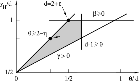
Figure 3: The domain of allowed values of $y_{H}=d-\beta/\nu$ and $y_{J}=\theta$. The arrow denotes the result of the perturbative expansion in $d=6-\epsilon$ dimensions. Most of the results for the exponents found numerically are located in the upper left corner

3.3 Renormalization group

Since $\theta>0$, it is plausible from Eq. 19, that in the critical region thermal fluctuations are less relevant than those of the frozen–in disorder. In a renormalization–group (RNG) treatment this feature is reflected in the existence of a $T=0$ fixed point, which is believed to describe the critical behavior of the random field Ising model.

Although there is so far no satisfying RNG analysis, we present here briefly a rough sketch of it, assuming a continuous transition up to $T=0$. We follow thereby closely the earlier work of Bray and Moore $\!{}^{{\bf?}}$. We start with the observation, that the free energy density $f$ can be written in the form $f=J{\tilde{f}}(T/J,h/J,H/J)$. Let us imagine to carry out the RNG coarse–graining transformation, with length scale factor $b$, corresponding to a reduction in the number of degrees of freedom by a factor $b^{d}$. The transformation generates a flow in the space of the naive scaling fields $T/J,\,\,h/J$, and $H/J$, which eventually terminates in one of the fixed points of the system. The existence of three fixed point will be assumed (Fig. 4), in addition to the trivial, high temperature fixed point:

(i) A totally unstable “thermal” fixed point $C$ at $T=T_{c}$, $H=h=0$ (the random field is a relevant perturbation, see our discussion in 3.2) .

(ii) A fixed point $R$ at $T=H=0$ and $h=h_{R}$ which is unstable in two, but stable in one directions and is therefore a critical point.

(iii) A totally stable fixed point $F$ at $T=h=H=0$, which corresponds to the low temperature phase for $d>d_{l}$.

Figure 4: Schematic renormalization group flow of the random field Ising model

In general the RNG procedure generates also new terms in the Hamiltonian. We will assume, that these terms are irrelevant in the RNG–sense and can therefore be neglected.

In order to calculate the critical behavior we have to linearize the RNG flow close to the fixed point $R$. The eigenvalues and eigenvectors of the linearized RNG–transformation deliver the critical exponents and scaling fields. Phenomenological arguments concerning the RNG flow suggest

$$\frac{T}{J},\quad\tau=\frac{1}{J}(h-h_{R})+c\frac{T}{J}\quad{\rm and}\quad\frac{H}{J}$$ (23)

as the scaling fields. Close to the fixed point $R$  $J$, $\tau$ and $H$ transform under the RNG coarse graining as

$$\begin{array}[]{ccc}J\rightarrow J^{\prime}&=&J\,b\,^{y_{J}}\\ \tau\rightarrow\tau^{\prime}&=&\tau\,b\,^{y_{\tau}}\\ H\rightarrow H^{\prime}&=&H\,b\,^{y_{H}}.\end{array}$$ (24)

From Eq. 23, Eq. 24 and the invariance of the partition function under the RNG transformation we get for the singular part of the free energy density $f=J\cdot{\tilde{f}}$

$${\tilde{f}}\left(\frac{T}{J},\tau,\frac{H}{J}\right)=b^{y_{J}-d}{\tilde{f}}\left(\frac{T}{J}b^{-y_{J}},\tau b^{y_{\tau}},\frac{H}{J}b^{y_{H}-y_{J}}\right)$$ (25)

and similar for the correlation length $\xi$

$$\xi\left(\frac{T}{J},\tau,\frac{H}{J}\right)=b\xi\left(\frac{T}{J}b^{-y_{J}},\tau b^{y_{\tau}},\frac{H}{J}b^{y_{H}-y_{J}}\right).$$ (26)

The critical exponents follow from Eq. 25 and Eq. 26 in the usual way, their relations to eigenvalue exponents $y_{i}$ are summarized in the following list:

$$\begin{array}[]{l@{\qquad}l@{\qquad}l}\beta=\nu(d-y_{H})&\nu=1/y_{\tau}&\theta=y_{J}\\ \gamma=\nu(2y_{H}-y_{J}-d)&\eta=2+d+y_{J}-2y_{H}&\\ \delta=(y_{H}-y_{J})/(d-y_{H})&\bar{\eta}=4+d-2y_{H}&.\end{array}$$ (27)

These scaling relations are in agreement with Eq. 17 and Eq. 22. The existence of a zero–temperature fixed point corresponds to a positive value of $y_{J}\equiv\theta$. Alternatively, $-y_{J}$ can be interpreted as the eigenvalue exponent of the temperature or, by simple scale transformation $\phi=\sqrt{T\phi^{\prime}}$ in Eq. 3, of the coupling constant $u$. With this interpretation of $-y_{J}$, the modified hyper-scaling law Eq. 17 has been first derived by Grinstein $\!{}^{{\bf?}}$. The RNG program scetched above has been performed in real space using Migdal-Kadanoff or related approximations by a number of groups $\!{}^{{\bf?},{\bf?},{\bf?},{\bf?}}$ (see Table 1).

3.4 Dimensional reduction and weighted mean field approximation

A convenient starting point to study the critical behavior is the Ginzburg–Landau Hamiltonian ${\cal H}_{\rm GL}\{\phi\}$. Including a random field term, Young $\!{}^{{\bf?}}$ was able to show that the most singular terms in the perturbation theory for this model follow then from tree diagrams, which can alternatively be obtained from an iterative solution of the saddle point equation

$$\delta{\cal H}_{\rm GL}/\delta\phi=-{\bf\nabla}\phi^{2}+V^{\prime}(\phi)-h({\bf r})=0.$$ (28)

Here $V(\phi)=\frac{1}{2}{\tilde{a}}\phi^{2}+\frac{1}{4}u\phi^{4}$. The contributions from tree diagrams lead to an exact relation between the critical exponents $\lambda_{i}^{({\rm RF})}(d)$ of the random field system in $d$–dimension and those of the pure model in $(d-2)$–dimensions

$$\lambda_{i}^{({\rm RF})}(d)=\lambda_{i}^{({0})}(d-2)$$ (29)

the so called dimensional reduction. This equality has been proven, starting from Eq. 28, also in a non–perturbative way $\!{}^{{\bf?}}$. Comparing Eq. 29 with eq. Eq. 17 yields $\theta=2$ in all dimensions. Since the lower critical dimension of the pure Ising model is $d_{l}^{({0})}=1$ one would conclude $d_{l}^{({\rm RF})}=3$, in disagreement with our findings from the previous Section.

Apparently, perturbation theory is inappropriate to deal with this type of disorder which is characterized by a large number of local minima in the energy landscape. Indeed, since the perturbation theory can be generated from Eq. 28, all saddle point solutions enter expectation values of physical quantities with the weight $\pm 1$, which is clearly the wrong way.

More recently Lancaster et al. $\!{}^{{\bf?}}$ proposed a weighted mean field theory which takes into account all solutions $m_{i}^{\alpha}$ of the mean field equations

$$\partial F/\partial m_{i}=-J{\left.\sum\right._{j}}^{(i)}m_{j}+T\,{\rm arctanh}\,m_{i}-h_{i}=0,\qquad i=1,...,N.$$ (30)

Here ${\left.\sum\right._{j}}^{(i)}$ denotes the sum over the nearest neighbors to the site $i$. $h_{i}$ is taken from a bimodal distribution. Thermodynamic quantities are then calculated as a sum over all mean field solutions $\alpha$ with the Boltzmann weight $\exp{(-F_{\alpha}/T)}/\left.\sum\right._{\alpha}\exp{(-F_{\alpha}/T)}$ where $F_{\alpha}=E_{\alpha}-TS_{\alpha}$ is the mean field free energy and

$$\begin{array}[]{rcl}&&E_{\alpha}=-\frac{1}{2}J\sum\limits_{<ij>}m_{i}^{\alpha}m_{j}^{\alpha}-\sum\limits_{i}h_{i}m_{i}^{\alpha}\\ &&\\ &&S_{\alpha}=-\sum\limits_{i}\frac{1}{2}\left\{(1+m_{i}^{\alpha})\ln{(1+m_{i}^{\alpha})}+(1-m_{i}^{\alpha})\ln{(1-m_{i}^{\alpha})}-2\ln 2\right\}\end{array}.$$ (31)

We note, that Eq. 30 is a lattice version of Eq. 28 with $V(m_{i})=-T_{c}m_{i}+T\,{\rm arctanh}\,m_{i}$ and $T_{c}=2{\rm d}J$. Since Eq. 30 represents the saddle points of $F_{\alpha}$ and thermal fluctuations are expected to be irrelevant for the critical behavior, in principle one should be able to calculate the true critical exponents from this approach (at least at sufficiently low temperatures). Starting from high temperatures $T>T_{c}^{({\rm pure})}$ there is typically only one solution to the mean field equation. Decreasing $T$ below a temperature $T^{\ast}>T_{c}$, the number of solutions starts to grow rapidly. For a $32^{3}$ periodic lattice and an accuracy $|m_{i}^{\alpha}-m_{i}^{\gamma}|\stackrel{{\scriptstyle>}}{{\sim}}10^{-3}$, this number becomes of the order 250, although the number of those with a large weight increases more slowly. The critical exponents obtained in this way are summarized in Table 1. Lancaster et al. $\!{}^{{\bf?}}$ identify $T^{\ast}$ with the temperature $T_{RSB}$, at which replica symmetry breaking occurs (see Section 3.6).

3.5 Two or three independent exponents ?

In contrast to conventional critical points, which are characterized by two independent critical exponents, our schematic renormalization group calculation suggests, that the random field Ising model is characterized by three independent exponents.

In an early publication, Aharony, Imry and Ma $\!{}^{{\bf?}}$ suggested the existence of an exact exponent relation

$$\theta=2-\eta$$ (32)

which implies $2\eta=\bar{\eta}$ and reduces the number of independent exponents again to two. Relation Eq. 32 can indeed be made plausible by estimating the free energy of a correlated droplet $F_{\xi}$ close to the critical point. With $M({\bf r})\approx\chi\,h\xi^{-d/2}\sim h\xi^{2-\eta-d/2}$ for the local magnetization, where $\chi=G({\bf 0})/T$ denotes the susceptibility, and Eq. 19 we get

$$F_{\xi}\sim\int_{{\bf r}\in\xi^{d}}{\rm d}^{d}r\,h({\bf r})M({\bf r})\sim h^{2}\xi^{2-\eta}\sim\xi^{\theta}$$ (33)

which gives Eq. 32. Later Schwartz et al. $\!{}^{{\bf?}}$ have claimed, that there is an exact proof for this relation. However, all these approaches use in one or the other way linear response arguments and have therefore to be considered with caution. Numerical calculations show, that Eq. 32 is indeed fulfilled within the accuracy of the calculation.

Since the numerical determination of exponents in random systems is typically hampered by the existence of considerable error bars, which makes a confirmation of Eq. 32 difficult, Gofman et al. $\!{}^{{\bf?}}$ considered the even stronger relation

$$A=\lim\limits_{T\rightarrow T_{c}}\frac{T^{2}}{h^{2}}\frac{C_{dis}({\bf 0})}{G^{2}({\bf 0})}=1$$ (34)

which should be fulfilled according to $\!{}^{{\bf?}}$.

The exponent scaling gives for $C_{dis}(0)/G^{2}(0)\sim\xi^{2\eta-\bar{\eta}}$, which would diverge (compare Eq. 18 and Eq. 27) unless Eq. 32 is valid. Gofman et al. determine $A$ from a 15 terms high temperature series expansion for $G(0)+C_{dis}(0)$ and $G(0)$ in $d=3,\,4,\,5$ dimensions for different values of the random field strength $h$. In particular, for $d=3$, $A=1\pm 0.003$ which is an impressive confirmation of Eq. 34 and Eq. 32 (but not a proof!). Thus, despite of all efforts to prove Eq. 32 this problem has still to be considered as unsolved.

Table 1: Critical exponents.

Reference	$\theta=y_{J}$	$\nu=1/y_{\tau}$	$\beta=\nu(d-y_{H})$	$2\eta-\bar{\eta}=\theta-2+\eta$
${\rm MFA}^{\,\,}$	$d-4$	1/2	$1/2$	$d-6$
${\rm PT}^{\,\,}$ $d=6-\epsilon$	2	$\nu^{({0})}(d-2)$	$\beta^{({0})}(d-2)$	$\eta^{({0})}(d-2)$
$d\rightarrow 2$	1	0	2	0
weighted MFA $\!{}^{{\bf?}}$	1.51	$1.25\pm 0.11$
${\rm{\bf MC}}^{\,\,}$ (d=3)
Rieger and Young $\!{}^{{\bf?}}$	$1.56\pm 0.1$	$1.6\pm 0.3$	$0.003\pm 0.05$	$0.12\pm 0.12$
Rieger $\!{}^{{\bf?}}$	$1.53\pm 0.1$	$1.1\pm 0.2$	$0.00\pm 0.05$	$-0.03\pm 0.15$
${\rm HTSE}^{\,\,}$ Gofman et al. $\!{}^{{\bf?}}$	$(\gamma=2.1\pm 0.2)$			0
Realspace RNG
Dayan et al. $\!{}^{{\bf?}}$ Newmann et al. $\!{}^{{\bf?}}$ Cao and Machta $\!{}^{{\bf?}}$ Falicov et al. $\!{}^{{\bf?}}$	1.56 $1.00\pm 0.05$ 1.5 $1.4916\pm 0.0003$	$1.39$ $1.49\pm 0.008$ $\nu=2.25$ $\nu=2.25\pm 0.01$	$\approx 0$ $1.66\pm 0.01$ 0.02 $0.0200\pm 0.0005$	0.12 1.24 0.02 $0.001\pm 0.001$

3.6 Replica symmetry breaking (RSB)

The disorder average can conveniently be performed using the replica trick. E.g. the average free energy can be written as

$$\bar{F}=-T\overline{\ln Z}=-T\lim\limits_{n\rightarrow 0}\frac{1}{n}(\overline{Z^{n}}-1)$$ (35)

where $\overline{Z^{n}}=\overline{({\rm Tr}\,\exp{(-{\cal H}/T)})^{n}}={\rm Tr}\,\exp{(-(1/T){\cal H}_{n}\{S_{i}^{\alpha}\})}$ is the conventional partition function of the translationally invariant replica Hamiltonian

$${\cal H}_{n}\{S_{i}^{\alpha}\}=-\sum\limits_{\alpha,\beta}\sum\limits_{i,j}\left(J_{ij}\delta_{\alpha\beta}+\frac{h^{2}}{2T}\delta_{ij}\right)S_{i}^{\alpha}S_{j}^{\beta}.$$ (36)

An alternative formulation uses the Ginzburg–Landau model as the starting point with the corresponding replica Hamiltonian

$${\cal H}_{GL,n}\{\phi^{\alpha}({\bf r})\}=\sum\limits_{\alpha}{\cal H}_{\rm GL}\{\phi^{\alpha}\}-\sum_{\alpha,\beta}\int{\rm d}^{d}r\frac{h^{2}}{2T}\phi^{\alpha}\phi^{\beta}.$$ (37)

Mezard and Young $\!{}^{{\bf?}}$ use an $m$–component generalization of Eq. 37, $\phi^{\alpha}({\bf r})\rightarrow\vec{\phi}^{\alpha}({\bf r})=(\phi_{i}^{\alpha}(r),i=1\ldots m)$, to determine the correlation functions $G^{\alpha\beta}({\bf k})$ and $C_{dis}^{\alpha\beta}({\bf k})$ from Bray’s self–consistent screening approximation (SCSA). Note, that this generalization changes the lower critical dimension from $d_{l}=2$ to $d_{l}=4$, which follows both from perturbation theory and, because of the continuous symmetry of the order parameter, also from the Imry-Ma argument $\!{}^{{\bf?}}$. However, dimensional reduction is expected to break down also in this case $\!{}^{{\bf?}}$.

The SCSA is a truncation of Dyson’s equation which is exact to order $1/m$. Assuming a replica–symmetric solution, Mezard and Young find the dimensional reduction result $\eta(d)=\bar{\eta}(d)=\eta^{(0)}(d-2)=O(1/m)$. This replica symmetric solution is however unstable with respect to RSB. Using the hierarchical RSB scheme of Parisi, they find $\eta=\eta^{(0)}(d-2)$ to order $1/m$, but the value $\bar{\eta}$ is now altered. The difference $2\eta-\bar{\eta}=c/m$ is small for any $m$. The constant $c$ can in principle be determined from the set of self–consistent equations. This calculation has been extended by Mezard and Monasson $\!{}^{{\bf?}}$ and de Dominicis et al. $\!{}^{{\bf?}}$, who determined the temperature $T_{\rm RSB}>T_{c}$, where the replica symmetric solution becomes unstable. In particular, de Dominicis et al. $\!{}^{{\bf?}}$ consider a more general coupling term $\left.\sum\right._{\bf k}\Delta_{\alpha\beta}({\bf k})\phi_{\bf k}^{\alpha}\phi_{-{\bf k}}^{\beta}$ between the replicas in Eq. 37 and determine $T_{\rm RSB}$ from the divergence of the $\Delta$–susceptibility $\partial^{2}\overline{Z^{n}}/\partial\Delta_{\alpha\beta}({\bf p})\partial\Delta_{\gamma\delta}({\bf p}^{\prime})$ (to reach this goal, in practice they use the Legendre–transform of $\overline{Z^{n}}$), which is related to the standard spin–glass susceptibility. It turns out, that the spin–glass transition (in the sense of an Almeida-Thouless line), which is believed to take place at $T_{\rm RSB}$, always precedes the ferromagnetic transition (see Fig. 5). For $d$ close to six dimensions they get in particular

$$|T_{\rm RSB}-T_{c}(h)|\approx J(h/J)^{8/(6-d)}.$$ (38)

This has to be compared with the Levanyuk–Ginzburg criterion, Eq.16, which gives a random field controlled critical region of size

$$|T_{\rm LG}-T_{c}(h)|\approx J(h/J)^{4/(6-d)}\gg|T_{\rm RSB}-T_{c}(h)|.$$ (39)

For $T_{c}<T<T_{\rm LG}$ we expect, that the saddle point equations Eq. 28, Eq. 30, will have several solutions, which signals the failure of perturbation and linear response theory. It is at present unclear, whether RSB (and hence the breakdown of dimensional reduction) occurs in the whole random field critical region, as one would naively expect and as was found in a more recent study by Dotsenko and Mezard $\!{}^{{\bf?}}$, or, as Eq. 38 suggests, is restricted to the much smaller temperature interval around $T_{c}(h)$ ($h\ll J$). We note finally, that the spin-glass order parameter $q_{EA}$ is non-zero at all temperatures. In particular, outside the critical region where linear response theory applies $\overline{<S_{l}>^{2}}=q_{EA}\approx\left.\sum\right._{ij}\chi_{li}\chi_{lj}\overline{h_{i}h_{j}}=h^{2}\left.\sum\right._{i}\chi_{li}^{2}>0$. Here $T\chi_{ij}=<S_{i}S_{j}>-<S_{i}><S_{j}>$ denotes the Fourier transform of $G({\bf k})$.

Although we have here only discussed the paramagnetic phase, one expects a similar behavior if one reaches the ferromagnetic transition line from below.

4 Dynamical Properties

4.1 Zero temperature interface depinning

At finite temperatures the two phases with up and down magnetization can coexist only for vanishing strength of the uniform external field $H=0$. This is not the case at zero temperature, where the disorder (and possibly also lattice effects) lead to a pinning of the wall separating the two domains. In order to get the wall depinned, the external field has to overcome a threshold $H_{c}$. Thus, the coexistence surface consists of two parts, for $0<T<T_{c}(h)$ it is restricted to $H=0$, whereas for $T=0$ it is given by $-H_{c}(h)\leq H\leq H_{c}(h)$ (see Fig. 5).

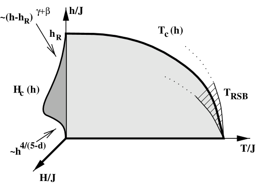
Figure 5: Coexistence surfaces of the random field Ising model

In this section we consider the behavior of the interface in the vicinity of the depinning threshold and determine $H_{c}$. The equation of motion of an over-damped wall is $\!{}^{{\bf?}}$

$$\lambda\frac{\partial z}{\partial t}=-\delta H_{I}/\delta z=\Gamma\underline{\nabla}^{2}\,z+2M(H+h(\underline{x},z)).$$ (40)

This equation is highly non-linear because of the last term on the rhs. $\lambda$ denotes the inverse mobility of the interface. We assume here, that the interface motion is over-damped. We will show later, that an inertial term is indeed irrelevant close to the depinning threshold. It turns however out, that it is important to assume a finite correlation length $a$ for the random field in the $z$–direction (which is the direction of motion of the interface), i.e. we replace Eq. 4 by

$$\overline{h(\underline{x},z)h(\underline{x}^{\prime},z^{\prime})}=h^{2}\delta^{\rm d-1}(\underline{x}-\underline{x}^{\prime})\Delta(z-z^{\prime})$$ (41)

with $\int_{-\infty}^{\infty}\Delta(z)=1$. $a$ is of the order of the lattice spacing, i.e. of order one in our units. $\Delta(z)=-\Delta(-z)$ is a monotonically decreasing function of $z$ for $z>0$ and decays rapidly to zero over a finite distance $a$. The width of the random field correlator perpendicular to $z$ turns out to be irrelevant, we assume therefore, that it is smaller than any other length of the problem.

The physics of the interface close to the depinning transition is characterized by two emerging important length scales, the Larkin length $L_{c}$ and the dynamical correlation length $\xi_{v}$. For weak disorder, $J\gg h$, $L_{c}$ is the length scale on which the typical distortion of the interface is of the order $a$. We have to compare here the curvature force $\Gamma L^{{\rm d}-3}a$ with the random force $\sim Mh\Delta^{1/2}(a)L^{{\rm(d-1)}/2}$ . In the case of weak disorder, which we consider here, $\Gamma a\gg Mh\Delta^{1/2}$, and the random force wins over the curvature force only on length scales

$$L>L_{c}\approx[(\Gamma a/Mh)^{2}/\Delta(a)]^{1/(5-{\rm d})}.$$ (42)

and ${\rm d}<5$. For $L<L_{c}$ (or ${\rm d}>5$), the interface is flat and hence cannot be pinned, since the total pinning force $\sim L^{{\rm(d-1)}/2}$ is always smaller than the driving force $\sim L^{\rm(d-1)}$. On the other hand, the interface is able to explore the inhomogeneous force field on larger length scales $L>L_{c}$. It follows, that the maximum pinning force on a piece of interface of linear dimension $L>L_{c}$ is of the order $(L/L_{c})^{\rm(d-1)}Mh[\Delta(a)L_{c}^{\rm(d-1)}]^{1/2}$, which leads to a threshold field of the order

$$H_{c}\approx\frac{1}{M}\Gamma L^{-2}_{c}a\approx\frac{\Gamma a}{M}\left[\left(\frac{hM}{\Gamma a}\right)^{2}\Delta(a)\right]^{2/(5-{\rm d})}.$$ (43)

For small $h$, $H_{c}\sim h^{4/(5-{\rm d})}$, i.e. $H_{c}\sim h^{2}$ in $d=3$ dimensions. Close to the critical point $h\stackrel{{\scriptstyle<}}{{\sim}}h_{R}$, $H_{c}\approx\Gamma\xi^{-1}/M\sim\tau^{\beta\delta}$. Note however, that $\Gamma$ carries its own $h$-dependence if Eq. 40 is derived from the bulk Hamiltonian (compare Section 2.3). Then for $h\rightarrow 0$, $H_{c}$ becomes exponentially small in $d=3$ dimensions.

To understand the nature of $\xi_{v}$, it is convenient to describe the interface in a co–moving frame $z(\underline{x},t)=h(\underline{x},t)+vt$ where $v=<\dot{z}>$ denotes the mean interface velocity. Hence

$$\lambda\frac{\partial h}{\partial t}=\Gamma\underline{\nabla}^{2}\,h+2MH-\lambda v+2Mh(\underline{x},vt+h).$$ (44)

Let us consider the motion of a domain wall over some typical obstacle formed by a random field cluster, which is assumed to be hit by the wall at $t=0$. For small $t$, the wall will locally be stopped whereas other parts will continue to move forward by a distance $vt$. If the moving wall behaves self–affine under the action of the random field (an assumption which we will prove later), it will form locally a bump of typical height $h\sim t^{\tilde{\zeta}/\tilde{z}}$, where $\tilde{\zeta}$ and $\tilde{z}$ are the non–equilibrium roughness and the dynamical index of the interface, respectively. Since $\tilde{\zeta}<\tilde{z}$, on time scales $t\gg t_{v}\sim v^{-\tilde{z}/(\tilde{z}-\tilde{\zeta})}$ we find $vt\gg h$ and hence the non–linearity in Eq. 44 can be neglected. On the time scale $t_{v}$ the local perturbation by the obstacle spreads out on the interface over a length scale

$$\xi_{v}\sim t_{v}^{1/\tilde{z}}\sim v^{-1/(\tilde{z}-\tilde{\zeta})}$$ (45)

which has apparently the meaning of a dynamical correlation length. Thus, on time and length scales $t\gg t_{v}$ and $L\gg\xi_{v}$, the effective interface equation is the linear Edwards-Wilkinson-equation $\!{}^{{\bf?}}$

$$\lambda_{\rm eff}\frac{\partial z}{\partial t}=\Gamma_{\rm eff}\underline{\nabla}^{2}z+2M(H_{\rm eff}+h_{\rm eff}(\underline{x},vt))$$ (46)

but with renormalized parameters. In particular, we will find $H_{\rm eff}=H-H_{c}$. In the rest of this section we determine the dependence of the effective parameters on $(H-H_{c})$ due to the non–linear effects on scales $L\ll\xi_{v}$. Once these dependencies are known, Eq. 46 can be treated easily, it yields in particular in $d=3$ dimensions a logarithmic roughness of the interface for $L\gg\xi_{v}$.

We start with the derivation of some scaling relations. If the transition from the moving to the pinned state of the interface is continuous, as we will show below, we expect a power law behavior of the velocity

$$v\sim(H-H_{c})^{\tilde{\beta}}$$ (47)

and hence $\xi_{v}\sim(H-H_{c})^{-\tilde{\beta}/(\tilde{z}-\tilde{\zeta})}$. One condition for a continuous transition follows from a Harris–like argument: the fluctuations $\delta H(\xi_{v})$ of the threshold force in the correlated volume $\xi_{v}^{{d-1}+\tilde{\zeta}}$ occupied by the rough interface should be small compared to $(H-H_{c})$  $\!{}^{{\bf?}}$. Thus, $(H-H_{c})\gg\delta H_{c}(\xi_{v})\sim\xi_{v}^{-({d-1}+\tilde{\zeta})/2}\sim(H-H_{c})^{\tilde{\nu}({d-1}+\tilde{\zeta})/2}$ or

$$\tilde{\nu}=\frac{\tilde{\beta}}{\tilde{z}-\tilde{\zeta}}\geq\frac{2}{{d-1}+\tilde{\zeta}}$$ (48)

where we introduced $\tilde{\nu}$ via $\xi_{v}\sim(H-H_{c})^{-\tilde{\nu}}$.

For large velocities the non–linear terms of Eq. 44 can be treated by standard perturbation theory  $\!{}^{{\bf?}}$. For the renormalized inverse mobility we obtain e. g.

$$\lambda_{\rm eff}=\lambda\left(1-c_{1}(\xi_{v}^{(0)}/L_{c})^{5-d}+c_{2}(\xi_{v}^{(0)}/L_{c})^{2(5-d)}-...\right).$$ (49)

Here $L_{c}$ is given by Eq. 42 with $\Delta(a)$ replaced by $|\Delta^{\prime\prime}(0)|a^{2}$ and $\xi_{v}^{(0)}=(\Gamma a/v\lambda)^{1/2}$ is the bare dynamical correlation length. Similar expressions can be obtained for the renormalization of $\Delta^{\prime\prime}(0)$. There is no renormalization of $\Gamma$, however, because of an exact tilt symmetry $\!{}^{{\bf?}}$.

The perturbation theory clearly diverges for $v\rightarrow 0$. It turns out, that a functional renormalization group calculation is required to find the true critical behavior since $\Delta^{\prime\prime}(0)$ develops a singularity under the renormalization group transformation if $b\approx L_{c}$. The resulting functional flow equation for the random–field correlator is

$$\frac{{\rm d}\Delta(z)}{{\rm d}\ln{b}}=(\tilde{\epsilon}-2\tilde{\zeta})\Delta(z)+\tilde{\zeta}z\Delta^{\prime}(z)-c\frac{{\rm d}^{2}}{{\rm d}z^{2}}\left[\frac{1}{2}\Delta^{2}(z)-\Delta(z)\Delta(0)\right]$$ (50)

where $\tilde{\epsilon}=5-d$. The fixed point function has a cusp–like singularity at the origin $\Delta^{\ast}(z)=\Delta(0)+a_{1}|z|+a_{2}z^{2}+\ldots$ where $a_{1}$ and $a_{2}$ are of the order $\tilde{\epsilon}$. It is important to note, that despite of the fact, that we were able to obtained $H_{c}$ in Eq. 43 from a simple scaling argument, the determination of $H_{c}$ from a straightforward calculation requires the existence of a non–zero value of $\Delta^{\prime}(z\rightarrow 0^{+})\sim H_{c}$. The roughness exponent $\tilde{\zeta}$ follows from the fixed point condition to be $\tilde{\zeta}=\tilde{\epsilon}/3$, which is identical with the equilibrium roughness exponent. The correlator of the effective random field $h_{eff}$, appearing in Eq. 46 is $\Delta_{eff}(z)\approx(L_{c}/\xi_{v})^{(\tilde{\epsilon}-2\tilde{\zeta})}\Delta^{\ast}(z(L_{c}/\xi_{v})^{\tilde{\zeta}})$.

The renormalization of the mobility is coupled to the renormalization of $\Delta_{eff}(z)$ and yields $\lambda_{eff}\sim(L_{c}/\xi_{v})^{2\tilde{\epsilon}/9}$. Together with the scaling relations $\!{}^{{\bf?}}$

$$\tilde{\nu}=\frac{1}{2-\tilde{\zeta}}$$ (51)

which is valid to all orders in $\tilde{\epsilon}$  $\!{}^{{\bf?}}$, this gives for the exponents to order $\tilde{\epsilon}=5-d$

$$\tilde{\zeta}\approx\frac{\tilde{\epsilon}}{3}\,,\quad\tilde{z}\approx 2-\frac{2}{9}\tilde{\epsilon}\,,\quad\tilde{\beta}\approx 1-\frac{\tilde{\epsilon}}{9}.$$ (52)

Narayan and Fisher $\!{}^{{\bf?}}$ have claimed, that $\tilde{\zeta}$ is correct to all orders in $\tilde{\epsilon}$, but numerical calculations show deviations from this result in low dimensions $\!{}^{{\bf?}}$. With these replacements, all terms in the Edwards-Wilkinson-equation Eq. 46 scale as $H-H_{c}$. It is easy to see, that at the depinning fixed point an inertial term is irrelevant since it scales as $(H-H_{c})^{\lambda}$ with $\lambda=1+2\frac{z-1}{2-\zeta}>1$.

Thermal fluctuations will smear out the transition such that the velocity is non–zero for all driving forces $HM$. For $H\approx H_{c}$

$$v\approx T^{\tilde{\beta}/\rho}\psi((H-H_{c})/T^{1/\rho})$$ (53)

with $\psi(x)\sim x^{\tilde{\beta}}$ for $x\rightarrow\infty$ and $\psi(x)\sim{\rm const}$ for $x\rightarrow 0$. The value of $\rho$ is at present unknown. For $H\ll H_{c}$, the velocity is exponentially small and results from a creep motion over the barriers formed by the random field

$$v\sim\exp{(-CMh^{2}/HT)}$$ (54)

with $C=O(1)$  $\!{}^{{\bf?}}$.

4.2 Critical dynamics

Villain $\!{}^{{\bf?}}$ and D.S. Fisher $\!{}^{{\bf?}}$ have proposed to consider the spin dynamics close to $T_{c}(h)$ as due to a kind of domain reversal, where now domains within domains should be taken into account through the exponent $\theta$ introduced in Eq. 17 and Eq. 19. The reversal of domain of size $\xi$ (the correlation length) is associated to an energy barrier of order $h\xi^{\theta}$, and the Arrhenius law gives the following expression of the relaxation time

$$t_{\rm rel}\approx\exp({\rm const.}\left|\frac{T_{c}}{T-T_{c}}\right|^{\nu\theta}).$$ (55)

This formula is in contrast with usual power laws and reminiscent of the Vogel–Fulcher law observed in amorphous systems $\!{}^{{\bf?}}$. We note, that conventional perturbation theory gives $t_{\rm rel}\approx|T-T_{c}|^{-\nu z}$ with dynamical critical exponent $z=2+2\eta$  $\!{}^{{\bf?}}$. Because of the exponential increase of the relaxation time, random field systems will rapidly fall out of equlibrium by approaching the transition.

4.3 Metastable domains

According to our finding of the Sec. 2.1, the $3$–dimensional random field Ising model should exhibit ferromagnetic order at low temperatures. Experiments on random field systems are mainly performed with diluted antiferromagnets in external field and show pronounced hysteresis effects  $\!{}^{{\bf?},{\bf?},{\bf?}}$. In particular, no long–range order is found for $3d$ systems cooled from the high–temperature phase in non–zero field $H$. Neutron scattering experiments in three dimensions yield a non-equilibrium correlation length

$$R_{c}(t)\sim H^{-\nu_{H}}\cdot r(t)\quad\mbox{with $\nu_{H}\approx 2.1-2.2$}.$$ (56)

The absence of long–range order has been traced back in these cases to domain wall pinning in metastable states $\!{}^{{\bf?},{\bf?},{\bf?}}$.

A short discussion of the domain relaxation ist found in $\!{}^{{\bf?}}$, which gives the following prediction for the non–equilibrium correlation length $\!{}^{{\bf?}}$

$$R_{c}(t)\approx\frac{\sigma\Gamma}{h^{2}}\left(C+\frac{T}{\Gamma}{\rm ln}(t/t_{0})\right)$$ (57)

where $C$ is a constant of order unity. This logarithmic growth has been seen experimentally $\!{}^{{\bf?}}$. In order to explain the experimental data of diluted antiferromagnets in an external field at low temperatures, it is necessary to take into account also pinning by random bonds $\!{}^{{\bf?}}$.

5 Miscellaneous

With the present review I have tried to summarize some of the more recent activities in the theoretical investigation of the Ising model in a random field. Clearly, because of limitation of space and time not all new and interesting developments found their place in this review.

To mention one, Dahmen, Sethna and co-workers $\!{}^{{\bf?}}$ have studied the zero temperature random field Ising model as a model for noise and avalanches in hysteretic systems. Changing the external field $H(t)$ adiabatically from its initial state where all spins point downwards, at small disorder (i.e. for small $h$) the first spin to flip easily pushes over its neighbors, and the transition happens in one burst (an infinite avalanche). On the other hand, at large enough disorder the coupling between spins becomes negligible, and most spins flip by themselves, no infinite avalanche occurs. Tuning the amount of disorder in the system, i.e. the random field strength $h$, one finds a non-equilibrium critical point ${\tilde{h}}_{c},{\tilde{H}}_{c}$ where infinite avalanches disappear. At this point there is a universal scaling law for the magnetization $m=M-M_{c}({\tilde{h}}_{c})$

$$m\approx|h-{\tilde{h}}_{c}|^{\beta}{\cal M}((H-{\tilde{H}}_{c})/(h-{\tilde{h}}_{c})^{\beta\delta}).$$ (58)

The critical exponents are believed to be those obtained for the equilibrium random field Ising model by dimensional reduction $\!{}^{{\bf?}}$. The relation between the critical field $H_{c}$ of Section 4.1 and ${\tilde{H}}_{c}$ is not clear at present.

Other work not mentioned in this review considers the Ising model in a random field in $d=1$ dimension or on special lattices, on which exact solutions are possible. I also left out the random field Ising model in a transverse field, the $m\rightarrow\infty$ limit of the random field Ising model etc.. We refer here the reader to the earlier review with P. Rujan $\!{}^{{\bf?}}$ or to the “Current Contents”.

The author of this review apologizes to all colleagues whose contribution has been omitted. He is conscious of its deficiencies, but nevertheless he hopes that it may be of some value for a first rough orientation in this field.

References

References

- [1] E. Ising, Z. Physik 31,253 (1925)
- [2] see e.g the contributions of H.N.V. Temperley and I. Syozi in “Phase Transitions and Critical Phenomena” ed. by C. Domb and M. S. Green, Vol.1, 227 (1972)
- [3] W. Selke, in “Phase Transitions and Critical Phenomena” ed. by C. Domb and J. Lebowitz, Vol.15,2 (1992)
- [4] P. Bak et al., J. Phys. C 18, 3911 (1985)
- [5] A. B. Harris, J. Phys. C 7, 1671 (1974)
- [6] K. Hui and A. N. Berker, Phys. Rev. Lett. 62, 2507 (1985), A. N. Berker, Physica A 194, 72 (1993)
- [7] see e.g. K. Binder and A. P. Young, Rev. Mod. Phys. 58, 801 (1986) for a review
- [8] Y. Imry and S.K. Ma, Phys. Rev. Lett. 35, 1399 (1975)
- [9] T. Nattermann and J. Villain, Phase Transition 11, 5 (1988); T. Nattermann and P. Rujan, Int. J. Mod. Phys. 3, 1597 (1989)
- [10] D. P. Belanger, Phase Transition 11, 53 (1988)
- [11] D. P. Belanger and A. P. Young, J. Magn. Mater 100, 272 (1991)
- [12] H. Rieger, “Monte Carlo studies of Ising spin glasses and random field systems” in: “ Annual Reviews of Computational Physics, ed. D. Stauffer”, p.295-342, World Scientific, Singapore 1995
- [13] S. Fishman and A. Aharony, J. Phys. C 12, L729 (1979) see also D. P. Belanger, this volume
- [14] J. Villain, J. Physique Lett (France) 43, 808 (1982)
- [15] P.G. de Gennes, J. Phys. Chem. 88, 6469 (1984), S. B. Dierker and P. Wiltzius, Phys. Rev. Lett. 58, 1865 (1987)
- [16] J. T. Graham et al., Phys. Rev B 35, 2098 (1987)
- [17] J. F. Fernandez, Europhys. Lett. 5, 129 (1988)
- [18] W. Fenzl and J. Peisl, Phys. Rev. Lett. 54, 2064 (1985)
- [19] C. Bostoen and K. H. Michel, Z. Phys. B 71, 369 (1988), see also T. Nattermann Ferroelectrics 104, 171 (1990) for further references
- [20] A. M. Gutin et al., cond–mat/9606136
- [21] T. R. Kirkpatrick and D. Belitz Phys. Rev. Lett. 74, 1178 (1995)
- [22] A. Beretti, J. Stat. Phys. 38, 483 (1985).
- [23] J. Fröhlich, in the 1984 Les Houches summer school, New York, Plenum
- [24] K. Binder, Z. Phys. B 50, 343 (1983).
- [25] M. Aizenman and J. Wehr, Phys. Rev. Lett. 62, 2503 (1989)
- [26] J.Z. Imbrie, Phys. Rev. Lett. 53, 1747 (1984); Comm. Math. Phys. 98, 145 (1985)
- [27] J T. Chalker, J. Phys. C 16, 6615 (1983), D.S. Fisher, J. Fröhlich and T. Spencer, J. Stat. Phys. 34, 863 (1984)
- [28] J. Bricmont and A. Kupiainen, Phys. Rev. Lett. 59, 1829 (1987); Comm. Math. Phys. , (1988)
- [29] T. Nattermann, J. Phys. A 21, L645 (1988)
- [30] T. Nattermann, J. Phys. C 16, 6407 (1983)
- [31] A. Aharony, Y. Gefen and Y. Shapir, J. Phys. C 15, 673 (1982)
- [32] M. Schwartz, J. Villain, Y. Shapir and T. Nattermann, Phys. Rev B 48, 3095 (1993)
- [33] T. Nattermann, Z. Phys. B 54, 247 (1983), Phys. Stat. Sol. (b) 132, 125 (1985),
- [34] D. S. Fisher, Phys. Rev. Lett. 56, 1964 (1986)
- [35] J. P. Bouchaud and A. Georges, Phys. Rev. Lett. 68, 3908 (1992)
- [36] V. Villain, J. Physique Lett (France) 43, L551 (1982), Grinstein and S. K. Ma Phys. Rev. Lett. 49, 685 (1982)
- [37] Y. C. Zhang, J. Phys. A 19, L941 (1986), T. Nattermann, Europhys. Lett. 4, 1241 (1987)
- [38] A. Aharony, Phys. Rev B 18, 3318 (1978)
- [39] A. P. Young and M. Nauenberg, Phys. Rev. Lett. 54, 2429 (1985)
- [40] A. F. Khurana et al., Phys. Rev. Lett. 54, 357 (1985), Phys. Rev. Lett. 55, 856 (1986)
- [41] H. Rieger and P. Young, J. Phys. A 26, 5279 (1993)
- [42] Gofman et al. Phys. Rev. Lett. 71, 1569 (1993), Phys. Rev B 53, 6362 (1996)
- [43] M. R. Swift et al. , preprint (1996)
- [44] H. E. Stanley, “Introduction to Phase Transitions and Critical Phenomena”, Clarendon Press, Oxford 1971
- [45] G. Grinstein, Phys. Rev. Lett. 37, 944 (1976)
- [46] J. Villain, J. Physique 46, 1843 (1985)
- [47] D. S. Fisher, Phys. Rev. Lett. 56, 416 (1986)
- [48] M. Schwartz and A. Soffer, Phys. Rev. Lett. 55, 2499 (1985)
- [49] M. Schwartz and A. Soffer, Phys. Rev. 33, 2069 (1986); M. Schwartz et al., Physica A 178, 6 (1991)
- [50] A. B. Harris, J. Phys. C 7, 1671 (1974), J. T. Chayes et al. Phys. Rev. Lett. 57, 2999 (1986)
- [51] A. J. Bray and M. A. Moore J. Phys. C 18, L927 (1985)
- [52] I. Dayan, M. Schwartz and A.P. Young, J. Phys. A 26, 3093 (1993)
- [53] M. E. J. Newman et al., Phys. Rev B 48, 16533 (1993)
- [54] M. S. Cao and J. Machta, Phys. Rev B 48, 3177 (1993)
- [55] A. Falicov, A. N. Berker and S. R. McKay, Phys. Rev B 51, 8266 (1995)
- [56] A. P. Young, J. Phys. C 10, L 257 (1977)
- [57] G. Parisi and N. Sourlas, Phys. Rev. Lett. 43, 744 (1979)
- [58] D. Lancaster, E. Mariani and G. Parisi, J. Phys. A 28, 3359–73 (1995)
- [59] A. Aharony, Y. Imry and S.–K. Ma, Phys. Rev. Lett. 37, 1364 (1976)
- [60] H. Rieger, Phys. Rev B 52, 5659 (1995)
- [61] M. Mezard and A. P. Young, Europhys. Lett. 18, 653 (1992)
- [62] D. S. Fisher, Phys. Rev B 31, 7233 (1985)
- [63] M. Mezard and R. Monasson, Phys. Rev B 50, 7199 (1994)
- [64] C. De Dominicis, H. Orland and T. Temesvari, J. de Physique I 5, 987–1001 (1996)
- [65] V. Dotsenko and M. Mezard, preprint cond-mat/9611017 (1996)
- [66] M. V. Feigel’man, Sov. Phys. JETP 58, 1076 (1983)
- [67] T. Nattermann, S. Stepanow, L. H. Tang and H. Leschhorn J. de Physique II 2, 1483 (1992)
- [68] S. F. Edwards and D. R. Wilkinson, Proc. R. Soc. London, Ser. A 381, 17 (1982)
- [69] O. Narayan and D. S. Fisher, Phys. Rev B 48, 7030 (1993)
- [70] H. Leschhorn et al., Annalen der Physik, in press (1997)
- [71] T. Nattermann, Phys. Rev. Lett. 64, 2454 (1990)
- [72] J. Joffrin, in “Ill-Condensed Matter” (North-Holland, 1979)
- [73] D. Boyanowsky and J. L. Cardy, Phys. Rev. B 27, 5557 (1983)
- [74] R. Bruinsma and G. Aeppli, Phys. Rev. Lett. 52, 1543 (1983)
- [75]
- [76] Q. Feng at al. Phys. Rev B 51, 15188 (1995)
- [77] T. Nattermann and J. Vilfan, Phys. Rev. Lett. 61, 223 (1988)
- [78] J. P. Sethna et al. Phys. Rev. Lett. 70, 3347 (1993), K. Dahmen and J. P. Sethna Phys. Rev. Lett. 71, 3222 (1993),