[

Nonlocality of Kohn-Sham exchange-correlation fields in dielectrics

Abstract

The theory of the macroscopic field appearing in the Kohn-Sham exchange-correlation potential for dielectric materials, as introduced by Gonze, Ghosez and Godby, is reexamined. It is shown that this Kohn-Sham field cannot be determined from a knowledge of the local state of the material (local crystal potential, electric field, and polarization) alone. Instead, it has an intrinsically nonlocal dependence on the global electrostatic configuration. For example, it vanishes in simple transverse configurations of a polarized dielectric, but not in longitudinal ones.

]

Ever since it became clear that electric polarization is indeed a well-defined bulk quantity in an insulating crystal [1, 2, 3, 4], the status of this electric polarization in the Kohn-Sham (KS) density-functional theory (DFT) [5, 6] has become a topic of considerable interest [2, 7, 8, 9, 10, 11, 12]. (Throughout this Letter, I refer to the exact version of DFT in which the true KS exchange-correlation (XC) functional is presumed known.) In Ref. [2] it was argued that the polarization of a crystalline insulator should be given exactly by DFT, on the basis that charge densities are given exactly, and that any errors in polarization would show up as errors in charge densities at surfaces or interfaces. Gonze, Ghosez and Godby (GGG) [7, 8] then pointed out that in order for the DFT polarization to be correct, the DFT XC potential would need to have a linear spatial variation (i.e, an “XC electric field” $\cal E_{\rm xc}$ would have to be present). They formulated a new version of DFT appropriate for crystalline insulators, in which the density $n({\bf r})$ and the electronic polarization ${\bf P}$ are shown to be uniquely related to the periodic part of the potential $\widetilde{V}({\bf r})$ and the electric field $\cal E$. This extended Hohenberg-Kohn (HK) [5] principle then allows the XC energy to be expressed as a functional of $n({\bf r})$ and ${\bf P}$, instead of just $n(\bf r)$ alone. Recently, Martin and Ortiz [12] have reformulated and extended this analysis. While agreeing with many of the conclusions of GGG, they nevertheless appear to express some doubts about the GGG interpretation of the XC field, preferring instead to focus on the HK and KS descriptions for the change in polarization connected to a change in field.

In this Letter, I present an analysis that clarifies the role of the XC field in the exact KS theory. I start by deducing the behavior of the XC potential for several simple configurations of a finite sample of spontaneously polarized dielectric material in vacuum. These examples illustrate misleading aspects of certain arguments given by the previous Refs. [2, 8, 12]. Briefly, it is now understood [7, 8, 12] that the local periodic charge density in some small region of the sample can be generated by any of a continuous family of KS potentials labeled by the choice of effective field $\cal E_{\rm eff}=\cal E+E_{\rm xc}$ or, equivalently, by the choice of electric polarization ${\bf P}_{\rm eff}$, in the same small region of the corresponding fictitious KS system. Based on Refs. [2] and [8], one might assume that the correct choice would be the one that makes the polarization correct, $\bf P_{\rm eff}=\bf P$; while in a naive approach one would make the choice $\cal E_{\rm eff}=E$, at least for the case ${\cal E}=0$. Here, I show that neither of the above choices is generally correct. Instead, the correct choice is inherently nonlocal, and depends upon the electrostatic configuration of the entire system. For example, for configurations in which $\bf P(r)$ is essentially longitudinal, the correct choice is ${\bf P}_{\rm eff}=\bf P$; but if essentially transverse, then ${\cal E}_{\rm xc}=0$; and for more complicated geometries, neither simple choice is correct. This ultra-nonlocality of the XC potential appears to be an inherent complicating feature of the exact DFT theory.

I begin by establishing some notation and reviewing some basic results of Refs. [7, 8, 12]. Consider a periodic insulating crystal with fixed lattice vectors specifying the unit cell, and an external electron potential consisting of a periodic and a linear part, $V({\bf r})=\widetilde{V}({\bf r})-e{\cal E}\cdot\bf r$. A tilde, as on $\widetilde{V}$, will be used to indicate a quantity having the periodicity of the unit cell, and $\cal E$ is a uniform electric field. As long as $\cal E$ is not too large, one can with very good precision identify a physical (although, strictly, metastable) state of the system, having periodic density, that is connected to the ${\cal E}=0$ ground state by slow adiabatic switching of $\cal E$ [12, 13, 14]. Letting $\widetilde{n}$ be this periodic density, we can then search for the non-interacting KS system for which the effective potential has the same linear part (same field $\cal E$) but periodic part $\widetilde{V}_{\rm eff}^{\rm KS}$. These relations are those of the conventional KS theory applied naively to the periodic system, and can be summarized as

$$\{\widetilde{V},{\cal E}\}\;\matrix{\phantom{x}\cr\longleftrightarrow\cr{\rm I}\cr}\{\widetilde{n},{\cal E}\}\;\matrix{\phantom{x}\cr\longleftrightarrow\cr{\rm NI}\cr}\{\widetilde{V}_{\rm eff}^{\rm KS},{\cal E}\}$$ (1)

(here ‘I’ and ‘NI’ indicate ‘interacting’ and ‘noninteracting’ respectively). Alternatively, one can identify the electronic polarization ${\bf P}$ of the true interacting system and search for the non-interacting system that correctly reproduces both $\widetilde{n}$ and $\bf P$; that is,

$$\{\widetilde{V},{\cal E}\}\;\matrix{\phantom{x}\cr\longleftrightarrow\cr{\rm I}\cr}\{\widetilde{n},{\bf P}\}\;\matrix{\phantom{x}\cr\longleftrightarrow\cr{\rm NI}\cr}\{\widetilde{V}_{\rm eff}^{\rm GGG},{\cal E}_{\rm eff}\}\;\;.$$ (2)

This is the approach of GGG [7, 8]. Unless dictated by symmetry, as for a centrosymmetric crystal in zero field, there is no reason to expect $\cal E_{\rm eff}=E$, any more than we expect some particular Fourier component of $\widetilde{V}_{\rm eff}$ to match that of $\widetilde{V}$. Thus, the “exchange-correlation field” defined as ${\cal E_{\rm xc}=E_{\rm eff}-E}$ is generally non-zero. (It is understood that ${\cal E}_{\rm xc}$ is not a true electric field, since it acts only on the electrons.) In either case, Eq. (1) or (2), it has to be supposed that the non-interacting system is also an insulator [15], and that the field $\cal E$ or $\cal E_{\rm eff}$ acting on this non-interacting insulator is again small enough so that a metastable state is well defined [14].

FIG. 1.: Sample geometries of a spontaneously polarized material. Details are given in text. (a) Cubic sample with spontaneous polarization along $+\hat{x}$, partially reduced by depolarization fields arising from surface charges. (b) Slab geometry in which surface charges ${\bf P}_{\rm tot}\cdot\hat{n}$ are precisely cancelled by appropriately chosen external planar charges $\mp\sigma_{0}$. (c) Geometry composed of four domains in such a way that $\nabla\cdot{\bf P}=0$.

Either procedure, Eq. (1) or (2), is perfectly sensible in the abstract, but we now have to investigate whether and how it might apply to the case of a more realistic non-uniform configuration of a dielectric material. Consider, for example, the three geometries sketched in Fig. 1; we consider first the electrostatic configuration of the physical (interacting) system for each case. Figure 1(a) shows a cubic sample of a spontaneously polarized material. For definiteness, let us take this material to be BaTiO₃ in the cubic perovskite structure with the atomic coordinates frozen as follows: the unit cell is ideal cubic, the Ba nuclei lie at the cube corners, the O nuclei lie on the cube face centers, and the Ti nuclei are displaced by a constant distance $\delta_{\rm Ti}=0.05\,$Å along $\hat{x}$ from the cube centers. This material retains a gap of several eV and has a spontaneous (zero-field) polarization ${\bf P}_{\rm tot}^{(0)}={\bf P}_{\rm ion}+{\bf P}^{(0)}$ with both components ${\bf P}_{\rm ion}$ (nuclear plus core) and ${\bf P}^{(0)}$ (valence electronic) lying along $+\hat{x}$ [16]. The geometry of Fig. 1(a) is such that the surface discontinuities in $\bf P_{\rm tot}(r)$ give rise to macroscopic surface charges on the left and right faces [17], generating an electric field that partially depolarizes the sample. Thus, the electronic polarization at the point A in Fig. 1(a) will be somewhat reduced from $P^{(0)}$. In the configuration of Fig. 1(b), this is avoided by placing infinitely thin sheets of additional external charge $\mp\sigma_{0}=\pm P_{\rm tot}^{(0)}$ on the left and right faces respectively, precisely canceling the depolarization field [18]. Thus, the macroscopic electric field vanishes at point B, and the electronic polarization at this point is just ${\bf P}=P^{(0)}\hat{x}$. Finally, Fig. 1(c) shows a different configuration in which the internal fields also vanish. This time the sample is comprised of four domains in which the displacements of the Ti nuclei are along $\hat{e}({\bf r})$ with $\hat{e}=+\hat{x}$, $-\hat{y}$, $-\hat{x}$, and $+\hat{y}$ in the top, right, bottom, and left domains, respectively. Clearly the solution is ${\cal E}({\bf r})=0$ since then ${\bf P(r)}=P^{(0)}\hat{e}(\bf r)$ and thus $\nabla\cdot{\bf P}_{\rm tot}=\nabla\cdot{(\bf P}_{\rm ion}+{\bf P})=0$, which is consistent with ${\cal E}=0$. Thus, the local conditions at point B of Fig. 1(b) and point C of Fig. 1(c) are identical: ${\cal E}=0$ and ${\bf P}=P^{(0)}\hat{x}$.

Of course it must be assumed that the samples in Fig. 1 are sufficiently large that macroscopic fields can be defined. So, when we speak of “point A,” we really refer to a region, large compared to atomic dimensions but small compared to sample dimensions, in which a periodic $\widetilde{V}$ and field $\cal E$ can be identified. But note, also, that for a macroscopic sample having the configuration of Fig. 1(a), the electrostatic potential difference between the left and right faces may greatly exceed the band gap, so that in principle the ground state would become metallic. However, in the context of dielectric theory one is again much more interested in the metastable [14] insulating state obtained by starting from a configuration without macroscopic electric fields, such as that of Fig. 1(b), and then adiabatically restoring the fields. Throughout this Letter it will always be assumed that both the physical and the fictitious KS systems are in such metastable states [19].

Let us now deduce what must be the behavior of $V_{\rm xc}(\bf r)$ for each of the configurations of Fig. 1. The dot labeled ‘A’ in Fig. 2 represents the values of the physical electric field $\cal E$ and polarization $P$ of the interacting system of Fig. 1(a) at point A. These determine the density $\widetilde{n}$ at point A, which must be reproduced by the fictitious KS system at point A. The dashed curve indicates the locus of values $({\cal E}_{\rm eff},P_{\rm eff})$ of the KS system that are consistent with each other and with this given $\widetilde{n}$. The choice of Eq. (1) corresponds to point A^′ (insisting that $\cal E_{\rm eff}=E$), while that of Eq. (2) corresponds to point A^′′ (insisting that $P_{\rm eff}=P$). Any point on the dashed curve generates the correct periodic density at A, and so is a candidate for the state of the KS system at A.

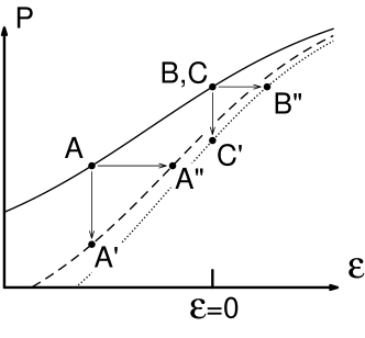
FIG. 2.: A, B, and C indicate the local state of the physical (interacting) system at corresponding points of Fig. 1; solid line is the dielectric relation for the physical material. A^′ and C^′ indicate states of the Kohn-Sham system having the correct density and field, Eq. (1); A^′′ and B^′′ indicate KS states having the correct density and polarization, Eq. (2). Dashed and dotted curves indicate the KS dielectric relations defined under the constraint that the periodic density match that of the physical system at A, or B and C, respectively.

Now comes the crucial point of the argument. In order to decide which point on this curve should be selected, it is necessary to inspect the configuration of the system as a whole. This is illustrated by the geometries of Fig. 1(b) and (c), for each of which the correct choice is easily deduced. As remarked above, in both cases the physical system is locally the same (point labeled ‘B,C’). For the geometry of Fig. 1(b), the translational symmetry[18] along $\hat{y}$ and $\hat{z}$ insures that both $\bf P$ and ${\bf P}_{\rm eff}$ lie along $\hat{x}$. But in either the physical (interacting) or the KS systems, the value of $\bf P$ is necessarily related [2] to the presence of a macroscopic electronic surface charge ${\bf P}\cdot\hat{n}$; and since this electronic charge must be given correctly in the KS theory, it is safe to conclude that ${\bf P}_{\rm eff}=\bf P$. Thus, for every point in the interior of Fig. 1(b), the state of the KS system is given by B^′′ in Fig. 2. On the other hand, in Fig. 1(c) both the physical and KS electric fields must vanish everywhere. Heuristically, this is suggested by the invariance of $V_{\rm eff}(\bf r)$ under fourfold rotation. More precisely, we can check that a consistent solution is obtained when, for every point in the interior of Fig. 1(c), the state of the KS system is given by C^′ in Fig. 2. In this case the polarization is given incorrectly by the KS theory at every interior point. Nevertheless, since $\nabla\cdot{\bf P}_{\rm eff}=0$ everywhere, such an error is still consistent with the KS system having exactly the correct $n({\bf r})$.

The example of Fig. 1(b) and (c) demonstrates that a knowledge of the local state of the physical interacting system (i.e., a knowledge of the material, and of $\cal E$ or equivalently of $\bf P$) is inherently insufficient to determine the corresponding local state of the KS system. Thus, a field ${\cal E}_{\rm xc}$ exists at point B, but not at point C, in spite of the fact that the local states of the physical systems at B and C are identical.

In general, the correct correspondence to the KS system must be determined by an analysis of the electrostatic configuration as a whole, and need not reduce to either simple choice (${\cal E}_{\rm eff}=\cal E$ or ${\bf P}_{\rm eff}=\bf P$). For example, for point A of Fig. 1(a), the correct choice of KS system might correspond to any of the points on the dashed curve of Fig. 2. To identify the correct point, an analysis of the following type would need to be carried through. Assuming that the physical $\cal E(\bf r)$ and $\bf P(r)$ are known: (i) At each point in space, obtain $\widetilde{n}$ from Eq. (1) or (2), and also obtain the dielectric relation ${\bf P}_{\rm eff}={\cal P}_{\tilde{n}}(\cal E_{\rm eff})$ for a non-interacting system constrained to have fixed $\widetilde{n}$ as $\cal E_{\rm eff}$ is varied (e.g., the dashed or dotted curve in Fig. 2). (ii) Taking first ${\cal E}_{\rm xc}=0$ (i.e., ${\cal E}_{\rm eff}=\cal E$) everywhere, compute the macroscopic charge density error $\delta n({\bf r})=\nabla\cdot[\bf P_{\rm eff}(r)-P(r)]$. (iii) Find a macroscopic field $\cal E_{\rm xc}(\bf r)$ such that, when acting on the system of nonlinear dielectric materials specified by dielectric responses ${\cal P}_{\tilde{n}}$, it induces precisely a cancelling charge density $-\delta n(\bf r)$.

The above is rarely a simple procedure in practice, but it illustrates the conditions under which a field $\cal E_{\rm xc}$ is needed. In Fig. 1(a) and (b), one finds $\delta n\neq 0$, so the XC field must be present; while for Fig. 1(c), $\delta n=0$ and so ${\cal E}_{\rm xc}=0$. In fact, it is evident that for a purely longitudinal configuration such as Fig. 1(b), Eq. (2) applies and the KS field $\cal E_{\rm eff}$ fails to match $\cal E$; while for a purely transverse configuration as in Fig. 1(c), Eq. (1) applies and instead the KS polarization $\bf P_{\rm eff}$ fails to match $\bf P$. It is easy to see that infrared-active longitudinal and transverse phonons in a polar insulator behave in a way analogous to Figs. 1(b) and (c), respectively.

A few comments may be in order. (i) According to the theory of Refs. [1, 2, 3, 4], the polarization $\bf P$ is actually only well-defined modulo $e{\bf R}/\Omega$, where $\bf R$ is a lattice vector and $\Omega$ is the cell volume. For the puposes of the arguments given here, we assume that the polarization differences [e.g., between domains in Fig. 1(c)] are sufficiently small that there is no difficulty in choosing the correct branch of $\bf P$. (ii) When constructing the KS potential for the configurations of Fig. 1, attention would also have to be given to the microscopic details of the choice of $V_{\rm xc}(\bf r)$ at surfaces and interfaces. However, local modifications to $V_{\rm xc}(\bf r)$ at a surface or interface will not affect the macroscopic electronic charge appearing there [2], so that the arguments about macroscopic fields will not be affected. (iii) In all of the arguments given here, the lattice coordinates have remained clamped. A realistic theory of dielectric materials would of course have to take into account the lattice relaxation effects.

In summary, it has been shown that the exact KS potential has an ultra-nonlocal dependence upon the electronic charge density, and this dependence does not take such a form that it can be automatically simplified by reference to the local electronic polarization. In some respects, the present conclusions are disappointing. One potentially appealing motivation for introducing [7, 8] the expanded HK correspondence $\{\widetilde{V},{\cal E}\}\leftrightarrow\{\widetilde{n},{\bf P}\}$, expressed explicitly in Ref. [12], is a hope that the generalized XC functional of density and polarization might be more localized than the conventional functional of density alone. The present conclusions unfortunately do not support this view. In fact, they reinforce previous indications that the true KS functional $V_{\rm xc}[n]$ is, in general, an extraordinarily non-local and irregular functional of the density [11]. As for the peculiar properties of $V_{\rm xc}[n]$ demonstrated here, there seems to be little hope of capturing these in practical approximations, even semilocal ones such as the weighted- or average-density approximations [20]. And indeed, it is not obvious that it would be desirable to do so. Of course, the approximate local and generalized-gradient functionals currently in use do not have these peculiarities.

This work was supported by NSF Grant DMR-96-13648. I wish to thank R.M. Martin for a conversation that stimulated the present work.

REFERENCES

- [1] R.D. King-Smith and D. Vanderbilt, Phys. Rev. B 47, 1651 (1993).
- [2] D. Vanderbilt and R.D. King-Smith, Phys. Rev. B 48, 4442 (1993).
- [3] R. Resta, Rev. Mod. Phys. 66, 899 (1994).
- [4] G. Ortiz and R.M. Martin, Phys. Rev. B 49, 14202 (1994).
- [5] W. Kohn and L.J. Sham, Phys. Rev. 140, A1133 (1965).
- [6] P. Hohenberg and W. Kohn, Phys. Rev. 136, B864 (1964).
- [7] X. Gonze, Ph. Ghosez and R.W. Godby, Phys. Rev. Lett. 74, 4035 (1995).
- [8] X. Gonze, Ph. Ghosez and R.W. Godby, Phys. Rev. Lett. 78, 294 (1997).
- [9] W.G. Aulbur, L. Jönsson, and J.W. Wilkins, Phys. Rev. B 54, 8540 (1996).
- [10] R. Resta, Phys. Rev. Lett. 77, 2265 (1996).
- [11] I.I. Mazin and R.E. Cohen, Ferroelectrics 194, 263 (1997).
- [12] R.M. Martin and G. Ortiz, Phys. Rev. B, in press.
- [13] G. Nenciu, Rev. Mod. Phys. 63, 91 (1991).
- [14] We shall say that a system in an electric field is metastable if the characteristic time for tunneling of electrons from valence to conduction states exceeds some long time (e.g., 103 yr).
- [15] As is well known, there are exceptions such as Ge, for which the KS system is metallic [see, e.g., R.W. Godby and R.J. Needs, Phys. Rev. Lett. 62, 1169 (1989)]. Such systems have to be excluded from the considerations given here.
- [16] R.D. King-Smith and D. Vanderbilt, Phys. Rev. B 49, 5828 (1994); W. Zhong, R.D. King-Smith, and D. Vanderbilt, Phys. Rev. Lett. 72, 3618 (1994).
- [17] It is also assumed here that the surfaces are insulating, so that the surface charge is related to the subsurface polarization in the obvious way. See also Ref. [2].
- [18] Fig. 1(b) is intended to suggest that the system extends indefinitely in the and directions. To be more conservative, we can let the system have large but finite dimensions in these directions.
- [19] Strictly speaking, it is also necessary to assume that the surfaces of the sample remain insulating.
- [20] O. Gunnarsson, M. Jonson, and B.I. Lundqvist, Phys. Rev. B 20, 3136 (1979).