Structure and apparent topography of TiO₂(110) surfaces

Abstract

We present self-consistent ab-initio total-energy and electronic-structure calculations on stoichiometric and non-stoichiometric TiO₂(110) surfaces. Scanning tunneling microscopy (STM) topographs are simulated by calculating the local electronic density of states over an energy window appropriate for the experimental positive-bias conditions. We find that under these conditions the STM tends to image the undercoordinated Ti atoms, in spite of the physical protrusion of the O atoms, giving an apparent reversal of topographic contrast on the stoichiometric 1$\times$1 or missing-row 2$\times$1 surface. We also show that both the interpretation of STM images and the direct comparison of surface energies favor an added-row structure over the missing-row structure for the oxygen-deficient 2$\times$1 surface.

]

I Introduction

Rutile TiO₂ has become something of a model system for the understanding of transition-metal oxide surfaces. In part this is because of the usefulness of TiO₂ as a support for transition-metal catalysts, and as a catalyst for photodissociation of water. But it also results from the fact that the TiO₂ (110) surface is relatively easy to prepare and characterize, and, for the stoichiometric surface at least, has a relatively simple surface structure. Considerable experimental information on this surface has been amassed using a variety of high-vacuum, surface-sensitive experimental techniques, including low-energy electron diffraction (LEED), electron energy loss spectroscopy (EELS), x-ray photoelectron spectroscopy (XPS), ultraviolet photoelectron spectroscopy (UPS), and inverse photoemission spectroscopy (IPE). [1] Among these surface-sensitive studies, scanning tunneling microscopy (STM) is the most natural and promising method to study atomic-scale structure on the surfaces. However, since STM is only sensitive to the local electronic density of states above the surface, it was not clear whether the bright rows observed on stoichiometric TiO₂(110) should correspond to physically raised (e.g., bridging oxygen) or depressed (e.g., undercoordinated Ti) surface features. In our previous work, in collaboration with Diebold et al.,[2] we concluded that the STM is imaging the undercoordinated Ti atoms. The apparent corrugation in the image is reversed from the physical one, and the imaging on the surface is dominated by electronic effects.

However, the interpretation of structures observed on oxygen-deficient TiO₂(110) surfaces remains somewhat inconclusive. Oxygen deficiency is easily induced on the surface by means of ion bombardment or controlled thermal annealing and quenching. For a neutral surface, this will leave electrons lying in states of Ti $d$ character at the bottom of the conduction band, making the surface metallic. These defect structures strongly affect the chemical and electronic properties of the oxide surfaces. Much experimental work has been directed towards imaging and characterizing these defects in recent years, [3, 4, 5, 6, 7, 8] but there are still many observed features that remain unexplained. For example, several authors report a 2$\times$1 reconstructed phase on the surface.[3, 4, 5, 6] A model having alternate bridging oxygen rows removed has been considered to explain these features.[3, 4, 7] However, such a model appears to be inconsistent with the observed registry of the bright rows on neighboring 1$\times$1 and 2$\times$1 domains, in view of the conclusion that one is imaging undercoordinated Ti atoms.[2, 3] Fisher et al. have proposed that not only the bridging oxygen rows, but also the Ti atoms underneath, are removed.[5] However, this model does not appear to be very well motivated, and in any case it has the same registry problem as for the missing-row model. Finally, Onishi et al. have proposed a model in which extra rows of oxygen-deficient Ti₂O₃ units are added on top of the surface, centered above the exposed Ti rows.[6] Evidently, some mass exchange with surface steps would be needed for this structure to arise during surface treatments leading to oxygen deficiency. However, this may well occur at elevated temperatures or with subsequent annealing, and the model has the advantage of being free of the registry problem.[2] Moreover, the model is also supported by recent experimental work.[9]

Theoretical work investigating these surface defect structures has so far been limited.[2, 10, 11, 12, 13, 14] We [2] carried out calculations on the 2$\times$1 oxygen-deficient surface by first-principles pseudopotential methods. However, we are unaware of corresponding calculations on the other models mentioned above. Thus, in the present work we extend our previous studies to include the added-row model of Onishi et al.[6] We not only find that this model is in good agreement with the STM observations, but also that it has a lower surface energy than the missing-row structure. Our work thus supports the identification of the added-row model to explain the observed 2$\times$1 reconstruction on the oxygen-deficient Ti(110) surface.

The plan of the paper is as follows. Section II gives a brief summary of the technique used to perform the calculations. In Secs. III and IV we summarize our work on the stoichiometric 1$\times$1 and oxygen-deficient missing-row 2$\times$1 (110) surfaces, respectively. In Sec. V we present the STM simulations of the added-row model proposed by Onishiet al.,[6] and discuss the interpretation of the STM images in view of our results on this and other competing models. We also present the calculated surface energies of different models in Sec. VI, and identify the energetically favored model. Finally, in Sec. VII we conclude by indicating what light we think our work has shed on the understanding of the surface structure of this material.

II Methods

Our theoretical analysis is based on first-principles plane-wave pseudopotential calculations carried out within the local-density approximation (LDA) following the methods of Ref. [14]. The pseudopotentials for Ti and O are those used in Ref. [14], and were generated using an ultrasoft pseudopotential scheme.[15] Periodic supercells containing 18 and 30 atoms were used to study the stoichiometric 1${\times}$1 surface, while 34-atom cells were used for the non-stoichiometric 2${\times}$1 surface and the added-row model. For all cases, special $k$-point sets were chosen to correspond to a 16-point set in the full Brillouin zone of the 1$\times$1 surface. Self-consistent total-energy and force calculations were used to relax the atomic coordinates until the forces were less that 0.1 eV/Å and then a band-structure run was carried out to obtain the valence and conduction-band electronic wave functions. These were used to analyze the local density of states (LDOS) in the vacuum region above the surface.

The information in the LDOS was then used to simulate STM images. Since virtually all useful atomic-resolution STM images on this surface are obtained under positive bias conditions, [2, 3, 4, 6] in which electrons are tunneling into unoccupied conduction-band states, we focus on the LDOS in the region of the lower conduction band. In rough correspondence with the experimental conditions, we integrated the LDOS over an energy window from 0 to 2 eV above the conduction-band minimum (CBM) to find a “near-CBM charge density.” (In practice, we simply summed the charge densities of unoccupied states falling in this energy range. For oxygen-deficient surfaces, where some electrons occupy conduction-band-like states, those occupied states were thus excluded from the sum.) For comparison, we also considered an energy window extending downwards by 1 eV from the valence band maximum (VBM) and thus obtained a “near-VBM charge density.”

As a technical point, it should be noted that our computed charge densities do not include the core augmentation contribution that appears as the second term in the expression

$$n({\bf r})=\sum_{i}\left[|\phi_{i}({\bf r})|^{2}+\sum_{nm,I}Q^{I}_{nm}({\bf r})\langle\phi_{i}|\beta^{I}_{n}\rangle\langle\beta^{I}_{m}|\phi_{i}\rangle\right]$$ (1)

for the electron density within the ultrasoft pseudopotential scheme.[15] For the STM simulations, only the first term describing the normal contributions of plane-wave components was included. The augmentation charge has been omitted in order to avoid unwanted spurious oscillations (“aliasing effects”) in the vacuum region resulting from the Fourier transform of a rapidly-varying core charge. The augmentation charge is strictly localized in the core regions (the core radii for Ti and O are about 1–2 a.u.) and so its omission does not in any way affect the LDOS in the vacuum region of interest for STM.

III The stoichiometric TiO₂ (110) surface

FIG. 1.: Ball-and-stick representations of the relaxed structures of the (110) surfaces investigated in this work. View is roughly along [001]. (a) Stoichiometric 1${\times}$1 surface. (b) Oxygen-deficient 2${\times}$1 missing-row model. (c) Oxygen-deficient 2${\times}$1 added-row model.

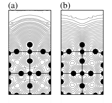
FIG. 2.: (a) Contour plots of [001]-averaged charge densities for the relaxed stoichiometric 1${\times}$1 surface. (a) Near-VBM charge densities obtained by integrating the LDOS over a 1-eV energy window near the valence band maximum. (b) Near-CBM charge densities obtained by integrating over a 2-eV energy window near the conduction band minimum. Contour levels correspond to a geometric progression of charge density, with a factor of 0.56 separating neighboring contours.

The relaxed structure of the stoichiometric TiO₂ (110) surface is shown in Fig. 1(a). The surface has rows of fivefold- and sixfold-coordinated Ti atoms along the bulk [001] direction. These are parallel to rows of twofold-coordinated oxygen atoms (bridging oxygen atoms) which are about 1.25Å above the surface. In our first-principles calculations, three-layer (18-atom) and five-layer (30-atom) periodic supercells were used, with the atomic positions relaxed to equilibrium. Both sizes of slab give very similar results for the LDOS in the vacuum region.

Contour plots of the $[001]$-averaged LDOS integrated over the VBM and CBM energy windows (see above) are shown in Fig. 2(a) and (b), respectively. Under constant-current tunneling conditions, the STM tip is roughly expected to follow one of the equal-density contours several angstroms above the surface. The contours of the near-VBM charge density shown in Fig. 2(a) follow the geometric corrugation closely, as would be expected from the dominance of the O $2p$ states around the VBM. However, the experimental conditions correspond to probing the unoccupied conduction-band states. Fig. 2(b) clearly shows that the contours of constant unoccupied near-CBM charge density extend higher above the 5-fold coordinated Ti atoms, in spite of the physical protrusion of the bridging oxygen atoms. This demonstrates that the STM is imaging the surface Ti atoms on the stoichiometric surface, i.e., that electronic-structure effects cause the apparent corrugation to be reversed from naive expectations. This is explained by the fact that the low-lying conduction-band states have a strong Ti $3d$ character,[14] leading to an enhancement of LDOS around the 5-fold coordinated Ti atoms. The apparent corrugation at a distance of 4-5 Å  above the surface is about 0.5-0.6 Å, in reasonable agreement with the experimentally observed results.

The two-dimensional variation of the near-CBM charge density is plotted for this surface in Fig. 3. The plane of the plot is 1.5 Å  above the bridging O atoms. This representation allows a more direct comparison with the actual STM images. The narrow bright stripes in the STM images should thus correspond with the elongated ridges visible in Fig. 3. The latter are located above the surface Ti rows.

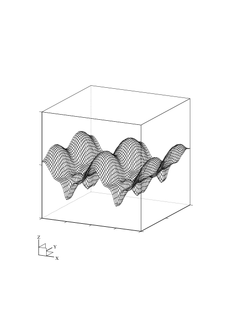
FIG. 3.: Near-CBM charge-density profile plotted in a surface (110) plane for four unit cells of the the stoichiometric 1$\times$1 surface. Here $x$ and $y$ label [$\bar{1}$10] and [001] respectively. The plane of the plot is located 1.5 Å  above the bridging oxygen atoms, the quantity plotted is actually averaged over 0.5 Å  along the [110] ($z$) direction, and the height of the plot is proportional to the logarithm of charge density.

IV The 2${\times}$1 missing-row model

The 2${\times}$1 missing-row structure is arrived at by removing alternate rows of bridging oxygen atoms. A fully relaxed model of this surface is shown in Fig. 1(b). The slab thickness and other theoretical details are the same as for the stoichiometric case.

The near-VBM charge density (not shown) again closely resembles the geometric corrugation of the surface, since once again the dominant contribution comes from the O $2p$ states. On the other hand, the near-CBM charge density, shown in Fig. 4, has a broad high-density feature above the missing bridging O atoms, and shows a depletion around the remaining O atoms. The corrugation of the constant-density contours is about 1Å. Again one finds that the apparent corrugation is the reverse of the geometric one, and that the calculation is consistent with the interpretation that the tunneling is enhanced by the strong Ti $3d$ character of the low-lying conduction-band states.[14] In fact, the tunneling is evidently especially strong into the 4-fold coordinated Ti atoms at the sites of the missing bridging O atoms. Clearly, the present results suggest that if the missing-row model were the correct one for the 2$\times$1 reconstructed phase, then the broad bright lines visible in STM images of this phase would correspond to the missing O rows – which, according to the results of the previous section, ought to coincide with the positions of the dark rows of the stoichiometric 1$\times$1 surface. However, this is not what is observed. Experimentally, the registry of the bright features of the 2$\times$1 structure coincides with that of the bright rows of the 1$\times$1 structure.[3, 8] Thus, our theory is not consistent with the missing-row model, and it is important to consider other models to explain the observed effects.

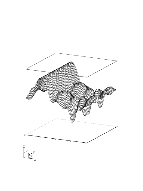
FIG. 4.: Near-CBM charge-density profile plotted in a surface (110) plane for two unit cells of the oxygen-deficient 2${\times}$1 missing-row structure. Details are as in Fig. 3; the vertical scale is identical to facilitate comparison.

V The 2$\times$1 added-row model

The relaxed structure of the added-row model[6] is shown in Fig. 1(c). Starting from the stoichiometric 1$\times$1 surface, this structure can be viewed as having been formed by the addition of extra rows of Ti₂O₃ units on top of alternate rows of five-fold coordinated Ti atoms. In this case, a two-layer, 34-atom periodic supercell was used in the calculation. The limited slab thickness is dictated by limitations of computational time and memory. In our calculation, we fixed the coordinates of the oxygen atoms in between the surface layers to their bulk values, in order to avoid a buckling of the slab that was otherwise induced by the strong surface relaxations. Other theoretical details are the same as for the previous cases.

Once again, the near-VBM charge density (not shown) follows the geometric corrugation of the surface fairly closely. The near-CBM charge density, shown in Fig. 5, exhibits a sharp increase around the position of the added Ti₂O₃ units, and the corrugation is about 1.5-2.0Å. The size of this corrugation is about the same as that of the defects reported by Novak et al.[3] This large corrugation is to be expected; apart from the physical protrusion of the added atoms above the surface, the added Ti₂O₃ units are themselves slightly non-stoichiometric.

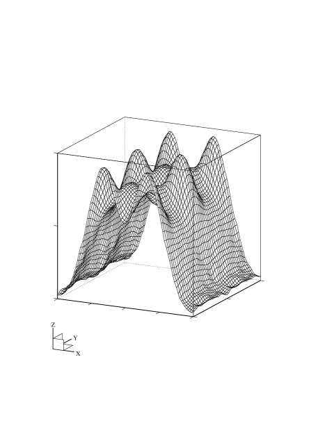
FIG. 5.: Near-CBM charge-density profile plotted in a surface (110) plane for two unit cells of the oxygen-deficient 2${\times}$1 added-row structure. Details are as in Fig. 3; the vertical scale is identical to facilitate comparison.

Moreover, unlike the missing-row model, the added-row model exhibits the expected registry between the features of the 2$\times$1 and 1$\times$1 phases. Consider a single isolated row of Ti₂O₃ units (sitting above five-fold coordinated Ti atoms as in the 2$\times$1 structure) on an otherwise stoichiometric 1$\times$1 surface. In the near-CBM charge density (and thus in the STM image) we would then expect a large peak at the position of the added row. Moreover, the five-fold coordinated Ti atoms on both sides of the added row will also contribute some peaks of corrugation of about 0.5Å. This corresponds closely with what is seen in the STM image as reported by Novak et al. [3]. In particular, all the peaks in the image are in registry with the five-fold coordinated Ti atoms. Therefore, this added-row model seems to be quite satisfactory for explaining the observed 2$\times$1 reconstruction, as well as the isolated bright lines, observed on the (110) surfaces.

As we shall see in the next section, the calculated surface energies also support the identification of the added-row model as the correct one for the 2$\times$1 surface. Since it is therefore likely to be of increasing theoretical and experimental interest, we have provided our relaxed coordinates for this model in Table I.

VI Energies of non-stoichiometric surfaces

We have also found the difference in surface energy between the oxygen-deficient 2${\times}$1 missing-row and added-row models. Fortunately, the two periodic supercells that we have used in the total-energy calculations for these models contain precisely the same numbers of Ti and O atoms, allowing a direct comparison of the energies. The added-row model is found to be 25.5 meV/Ų, or 0.97 eV per 2${\times}$1 surface cell, lower in energy than the missing-row surface. Therefore, besides solving the registry problem of the STM images, the added-row model is also energetically more favorable than the missing-row surface.

TABLE I.: Relaxed coordinates for the 2$\times$1 added-row structure. Only symmetry-distinct atoms in the added row and in the original top layer are listed; $x$, $y$, and $z$ are [$\bar{1}$10], [001] and [110] directions respectively. Units are 12.21a.u., i.e., the long dimension of the 1$\times$1 surface cell.

	$x$	$y$	$z$
Ti	$0.0$	$\,\,0.0$	$\,\,0.0$
	$0.276$	$\,\,0.0$	$\,\,0.395$
	$0.512$	$-0.227$	$\,\,0.009$
	$1.00$	$\,\,0.0$	$-0.022$
O	$0.0$	$\,\,0.0$	$\,\,0.319$
	$0.200$	$-0.227$	$\,\,0.029$
	$0.311$	$-0.227$	$\,\,0.547$
	$0.494$	$\,\,0.0$	$\,\,0.211$
	$0.809$	$-0.227$	$\,\,0.029$

Following Sec. V of Ref. [14], we also consider the possible phase separation of either the 2${\times}$1 missing-row or the added-row structure individually into equal areas of two kinds of 1$\times$1 domain, one with all the bridging oxygen atoms present [Fig. 1(a)] and the other with all bridging oxygen atoms missing. The energy difference for phase separation is calculated by comparing with the average of the surface energies for the stoichiometric 1$\times$1 and defective 1$\times$1 surfaces. Our slabs for these 1$\times$1 surfaces contain 18 and 16 atoms respectively, so that the total is again 34 atoms, and the numbers of Ti and O atoms are again identical with both of the 2${\times}$1 slabs. Therefore, the relative energies are again independent of any detailed knowledge of the Ti and O chemical potentials. We find that the 2$\times$1 missing-row and added-row surfaces are both stable with respect to phase separation, by approximately 6 and 32 meV/Ų, respectively.

VII Summary

We have studied a number of supercells to model both stoichiometric and non-stoichiometric (110) surfaces. From the results on the stoichiometric surface, we conclude that the narrow bright stripes observed in STM topographs correspond to the rows of five-fold coordinated Ti atoms. Due to the nature of the STM imaging technique, the STM is thus actually imaging the low-lying conduction band states with strong Ti $3d$ character. For the case of the oxygen-deficient 2${\times}$1 missing-row surface, on the other hand, we predict a strong accumulation of charge around the sites of the missing bridging oxygen atoms. This should appear as broad bright lines in the STM. However, while such lines are indeed observed for the experimental 2${\times}$1 phase, the registry of these lines with respect to the bright rows of the 1${\times}$1 domains is in conflict with the theory. The other reconstructed 2${\times}$1 model considered here is the added-row structure, for which we carried out similar calculations. We find that that the predicted STM image for this model now has the correct registry, giving rise to a broad peak in the near-CBM charge density above the added-row sites. We also find that the added-row model has a lower surface energy than the missing-row model. Therefore, we conclude that the added-row model appears to be a satisfactory model for describing the oxygen-deficient 2${\times}$1 TiO₂ surface reconstruction.

Further work is needed to resolve the interpretation of other features observed in STM images for oxygen-deficient TiO₂ (110) surfaces. For example, as pointed out by Diebold et al.,[2] point defects that are most likely single oxygen vacancies are observed on slightly reduced surfaces. Total-energy calculations for a supercell containing an isolated missing bridging oxygen atom would be very useful for confirming this identification. However, we have not pursued such a calculation because of the rather severe computational demands that were found to be necessary to obtain the needed accuracy.

- [1] V. E. Henrich and P. A. Cox, The Surface Science of Metal Oxides (Cambridge University Press, 1994).
- [2] U. Diebold, J. F. Anderson, K. O. Ng and D. Vanderbilt, Phys. Rev. Lett. 77, 1322 (1996).
- [3] D. Novak, E. Garfunkel, T. Gustafsson, Phys. Rev. B 50, 5000 (1994).
- [4] P. W. Murray, N. G. Condon and G. Thornton, Phys. Rev. B 51 (1995) 10989.
- [5] S. Fischer, A. W. Munz, K.-D. Schierbaum and W. Göpel, Surf. Sci. 337 (1995) 17.
- [6] H. Onishi and Y. Iwasawa, Surf. Sci. 313 (1994) L783; H. Onishi, K. Fukui and Y. Iwasawa, Bull. Chem. Soc. Jpn. 68 (1995) 2447; H. Onishi and Y. Iwasawa, Chem. Phys. Lett. 226 (1994) 111; H. Onishi and Y. Iwasawa, Phys. Rev. Lett. 76 (1996) 791.
- [7] A. Szabo and T. Engel, Surf. Sci. 329 (1995) 241; M. Sander and T. Engel, Surf. Sci. Lett. 302 (1994) L263.
- [8] P. J. Møller and M. C. Wu, Surf. Sci. 224 (1989) 265.
- [9] Q. Guo, I. Cocks, and E. M. Williams, Phys. Rev. Lett. 77 , 3851 (1996).
- [10] P. J. D. Lindan, N. M. Harrison, J. A. White and M. J. Gillan, Phys. Rev. B (in press)
- [11] O. Gülseren, R. James and D. W. Bullett, Surf. Sci. 377-379, 150 (1997)
- [12] M. Tsukada, H. Adachi and C. Satoko, Prog. Surf. Sci. 14, 113 (1983).
- [13] S. Munnix and M. Schmeits, Phys. Rev. B 31, 3369 (1985).
- [14] M. Ramamoorthy, R. D. King-Smith and D. Vanderbilt, Phys. Rev. B 49, 7709 (1994).
- [15] D. Vanderbilt, Phys. Rev. B 41, 7892 (1990).