Asymptotics of the trap-dominated Gunn effect in p-type Ge

Abstract

We present an asymptotic analysis of the Gunn effect in a drift-diffusion model—including electric-field-dependent generation-recombination processes—for long samples of strongly compensated p-type Ge at low temperature and under dc voltage bias. During each Gunn oscillation, there are different stages corresponding to the generation, motion and annihilation of solitary waves. Each stage may be described by one evolution equation for only one degree of freedom (the current density), except for the generation of each new wave. The wave generation is a faster process that may be described by solving a semiinfinite canonical problem. As a result of our study we have found that (depending on the boundary condition) one or several solitary waves may be shed during each period of the oscillation. Examples of numerical simulations validating our analysis are included.

I Introduction

In recent years a great variety of oscillatory behaviors have been observed in semiconductors displaying nonlinear electrical conduction. A particularly interesting system to study spatiotemporal phenomena in the laboratory is ultrapure extrinsic cooled bulk p-type Ge under voltage bias conditions, [6, 7]. Observed phenomena include time-periodic oscillations of the current on a purely resistive external circuit under dc voltage bias due to the periodic creation of a solitary wave at the injecting contact, its motion inside the semiconductor and its annihilation at the receiving contact [7]. Essentially this is the same as the usual Gunn effect in n-GaAs [8], except that the solitary wave in p-Ge moves much more slowly than the carriers (the case in the usual Gunn effect) due to the generation-recombination dynamics of ionized traps which dominate the transport properties. Other experimental observations include intermittency near the onset of the oscillatory instability [9, 10], and spatiotemporal chaos under dc$+$ac voltage bias [11]. These phenomena have been studied theoretically by means of a drift-diffusion model which includes impurity trapping of mobile holes and impact ionization of neutral acceptors [12, 13]. In dimensionless form, the model equations are [14]:

$$\frac{\partial A}{\partial t}=\frac{\Gamma}{\beta}\,(\alpha-1-A)+P\left[(\alpha-1)K(E)\right.$$ (1)

$$\left.\mbox{}-R(E)-[K(E)+R(E)]\,A\right],$$ (2)

$$\beta\frac{\partial E}{\partial t}=J-V(E)P+\delta\frac{\partial P}{\partial x},$$ (3)

$$\frac{\partial E}{\partial x}=P-A,$$ (4)

$${1\over L}\,\int_{0}^{L}E(x,t)\ dx=\phi.$$ (5)

The unknowns in these equations are the electric field $E(x,t)$, the hole concentration $P(x,t)$, the concentration of the ionized acceptors $A(x,t)$ and the total current density $J(t)$. $\phi$ is the constant dc bias. To solve this system of equations, we need two boundary conditions (representing the effect of the contacts at $x=0$ and $x=L$) and two initial conditions. In Section II we shall prove that we have a well-posed problem with positive solutions for all time for the following Dirichlet boundary conditions:

$$P(0,t)=P_{0},\quad\quad P(L,t)=P_{1}.$$ (6)

(the $P_{i}$’s are positive numbers). These conditions have been considered before in [15]. A discussion of imperfect boundary conditions for the Gunn effect introducing the concept of contact characteristic was first published by H. Kroemer [16]. Ohmic boundary conditions in which the field at the contact is proportional to the current density may give rise to negative current densities and numerical instabilities as time elapses. Eq. (2) is a rate equation for the ionized acceptors including the processes of photogeneration, impact ionization and recombination (coefficients $\Gamma$, $K(E)$ and $R(E)$, respectively). Eq. (3) is a form of Ampère’s law saying that the displacement current is equal to the total current density minus the drift-diffusion current due to the free holes. (4) is the Poisson equation and Eq. (5) is the voltage bias condition. The transport coefficients $V(E)$, $K(E)$ and $R(E)$ depend nonlinearly on the electric field as shown in Fig. 1 [13]. The qualitative nature of much of the predicted behavior—e.g., the instability of the stationary electric-field profile and the stability of propagating high-field domains—depends only on the presence of a negative slope of the homogeneous stationary current density $j(E)$ (defined below) over an interval of positive fields, [14, 17] and not on the exact form of the underlying coefficients. Other authors have stated different forms of the coefficient curves for various reasons.[18, 19, 20] Recently, Monte Carlo simulation has been used to provide a more rigorous determination of the coefficients for a related p-type system,[21] however such simulations do not yet exist for the closely compensated Ge samples under consideration in this paper. The homogeneous stationary current density $j(E)$ is given by the formula

$$j(E)=\left(\frac{\alpha K(E)}{K(E)+R(E)}-1\right)\,V(E),$$ (7)

[14, 22, 23]. If the compensation ratio $\alpha$ (the ratio of the acceptor concentration to the donor concentration) is only slightly larger than 1 (see [24] for the details), $j(E)$ is N-shaped for large enough positive fields. Then there is an interval $(E_{M},E_{m})$ between the abcissas of the maximum [$j(E_{M})=j_{M}$] and the minimum [$j(E_{m})=j_{m}>0$] of $j(E)$ for which $dj/dE<0$ and $j(E)>0$. See Fig. 1.

The dimensionless parameters $\beta$, $\delta$, and $\Gamma/\beta$ are very small for the p-Ge and can be set to zero in the leading order approximation [14]. Then $P=J/V(E)$ from (3), and (2) and (4) become:

$$\frac{\partial A}{\partial t} = {J\,[K(E)+R(E)]\over V(E)^{2}}\,[j(E)-V(E)\,A],$$ (8)

$$\frac{\partial E}{\partial x} = {J\over V(E)}-A.$$ (9)

Using Eq. (9), we may eliminate $A$ in favor of $E$ and then insert the result into (8). We obtain the following reduced equation [25, 14, 26]:

$$\frac{\partial^{2}{E}}{\partial{x}\partial{t}}+J\,\frac{K(E)+R(E)}{V(E)^{2}}\,\left(\frac{V^{\prime}(E)}{K(E)+R(E)}\,\frac{\partial E}{\partial t}\right.$$ (10)

$$\left.+V(E)\,\frac{\partial E}{\partial x}+j(E)-J\right)=\frac{1}{V(E)}\,\frac{dJ}{dt},$$ (11)

The reduced model equations (11) and (5) for $E(x,t)$ and $J(t)$ are supplemented with the boundary condition at the injecting contact $J(t)=P_{0}\,V[E(0,t)]$. According to this equation, the electric field at the contact is a nonlinear function of the current. In [26] it was shown that the resulting stable current oscillations are qualitatively like the solutions of the same reduced problem with the linear relation:

$$E(0,t)=\rho J(t),$$ (12)

(Ohm’s law; $\rho>0$ is the dimensionless contact resistivity) and an initial condition $E(x,0)$. Although much work has been done on the reduced model problem (11), (5) and (12) [see [23] and references therein; equivalently we may analyze (8), (9), (5) and (12)], important basic questions concerning the asymptotic description of their stable solutions are still open. In this paper we present an asymptotic description of the Gunn effect in p-Ge and compare the results with numerical simulations.

The paper is organized as follows. Section II contains a proof of the global existence of positive solutions to the full drift-diffusion model with particular boundary conditions and a brief review of the known results for the reduced model equations. In Sec. III, we introduce our asymptotic scaling, derive the outer and inner solutions, and put the pieces together thereby describing one period of the solution through the succession of its different stages. The delicate problem of shedding new waves through an instability of the boundary layer near the injecting contact is discussed in Section IV. Sec. V contains our conclusions and some open problems. Appendix A contains technical details on the shedding problem.

II Model system and global existence and uniqueness of solutions

We shall next show that, under rather mild assumptions on coefficients and data, the system (2)-(7) has a unique global solution when supplemented with initial conditions

$$A(x,0)\,=\,A_{0}(x),\qquad P(x,0)\,=\,\overline{P}(x).$$ (13)

Specifically, we will require functions $A_{0}$, $\overline{P}$, $P_{0}$ and $P_{1}$ ($P_{0}$ and $P_{1}$ may be known functions of time, not just constants) to be bounded, whereas functions $K(E)$, $R(E)$ and $V(E)$ will be assumed to be $C^{1}$. Furthermore, we shall impose the following growth condition on $K(E)$:

$$\left|K(E)\right|\,\leq\,C\left(\left|E\right|^{\gamma}\,+\,1\right)\quad\mbox{ for some }\gamma>0$$ (14)

(which is perfectly reasonable in view of the physics behind the model; see [23, 24]).

Without loss of generality, we may assume $P_{0}=P_{1}=0$ in (7), and $\Gamma=0$ in (2). As a matter of fact, the term thus dropped in (2) is a linear one and therefore harmless from the point of view of global existence. For the sake of notational simplicity, we shall also write:

$$f(A,E)=(\alpha-1)K(E)-R(E)-[K(E)+R(E)]\,A.$$ (15)

Differentiating (3) with respect to the space coordinate $x$ and using (4), we find the equation of charge continuity:

$$\beta\,P_{t}\,=\,\delta P_{xx}\,-\left(V(E)\,P\right)_{x}\,+\,\beta\,A_{t},$$ (16)

which is equivalent to

$$\beta\,P_{t}\,=\,\delta P_{xx}\,-\left(V(E)\,P\right)_{x}\,+\,\beta\,f(A,E)\,P,$$ (17)

once (2) is substituted into (16). Let us discuss first local existence of solutions. To this end, we observe that on setting $\psi=-\int_{0}^{x}E(\xi,t)d\xi$ (the electric potential), equations (4) and (7) read:

$$-\psi_{xx}\,=\,P\,-\,A;\qquad\psi(0,t)\,=\,0,\quad\psi(L,t)\,=\,-\phi\,L$$

By classical results for Poisson’s equation, we then deduce that:

Lemma 1. If $P$ and $A$ are bounded, then $\left|E_{x}\right|\,=\,\left|\psi_{xx}\right|\,\leq\,C$ for any $t\,>\,0$, where $C$ depends only on the bounds for $P$ and $A$.

On the other hand, integrating in (4) gives:

$$E\,=\,\int_{0}^{x}\,\left[P(\xi,t)\,-\,A(\xi,t)\right]\,d\xi\,+\,C_{1},$$

where $C_{1}\,=\,C_{1}(\phi,P,A)$. Hence, equation (17) may be rewritten in the form:

$$\beta\,P_{t}\,=\,\delta P_{xx}\,-\left(V(E)\,P\right)_{x}\,+\,\beta\,f(A,E(P,A))\,P$$ (18)

$$\qquad\equiv\,\delta P_{xx}\,+\,{\cal M}(P,P_{x},E,E_{x},A),$$ (19)

where the operator ${\cal M}$ is locally Lipschitz in its arguments. To proceed further, we remark that an integration in time of (2) yields

$$A(x,t)=A(x,0)+\int_{0}^{t}f[A(x,s),E(P,A)]\,P(x,s)ds$$ (20)

In view of (18) and (20), local existence follows now by means of a contractive fixed point argument for the following operator:

$$T\left(\begin{array}[]{c}P\\ \\ A\end{array}\right)=\left(\begin{array}[]{l}\frac{\delta}{\beta}S(t)\overline{P}+\frac{1}{\beta}\int_{0}^{t}S(t-s){\cal M}(P,P_{x},E,E_{x},A)ds\\ \\ A(x,0)\,+\,\int_{0}^{t}f(A(x,s),E(P,A))\end{array}\right)$$ (21)

where $S(t)$ denotes the heat semigroup in $[0,L]$ with homogeneous Dirichlet conditions. The operator $T$ is to be considered as acting on the space of functions $(P,A)$ such that $P\in L^{\infty}(0,t^{*};H^{1}(0,L))$ and $A\in L^{\infty}(0,t^{*};L^{\infty}(0,L))$, where $t^{*}$ is a sufficiently small positive number. On using the standard estimate

$$\|S(t)\,P\|_{H^{1}(0,L)}\,\leq\,C\,t^{-1/2}\,\|P\|_{L^{2}(0,L)}$$

for some $C>0$ (see for instance [27]), we readily derive the contractivity of the operator $T$ for $0<t^{*}\ll 1$. This gives at once local existence and uniqueness. We next set out to describe our global existence argument. To that end, we shall first prove that the following result holds for (16):

Lemma 2. Assume that $A(x,t)$ and $\overline{P}(x)$ are bounded. Then for any $\alpha_{1}>1$ there exists $C=C(\alpha_{1})>0$ such that

$$\left(\int_{0}^{t}\,\int_{0}^{L}\,\left|P(x,t)\right|^{\alpha_{1}}\,dx\,dt\right)^{1/\alpha_{1}}$$ (22)

$$\leq\,C\,\left(\|A\|_{\infty}\,(t+1)\,+\,\|\overline{P}\|_{\infty}\right),$$ (23)

for any $t>0$ for which a solution of our problem exists.

We remark in passing that we are denoting by $\|A\|_{\infty}$ a bound on the supremum of $A$. To prove Lemma 2, we argue as follows. Set

$$u\,=\,\int_{0}^{t}\,P(x,s)\,ds$$ (24)

Then $u$ satisfies

$$\beta\,{\partial u\over\partial t} = \delta\,{\partial^{2}u\over\partial x^{2}}+\beta\,A(x,t)$$ (25)

$$- \frac{\partial}{\partial x}\left(\,\int_{0}^{t}\,V(E(x,s))\,P(x,s)\,ds\,\right).$$ (26)

If the last terms on the right of (21) were absent, standard parabolic theory would yield at once

$$\left(\,\int\int_{Q}\,|u_{t}|^{\alpha_{1}}\,dx\,dt\right)^{1/\alpha_{1}}\,\leq\,C\,\left(\|A\|_{\infty}\,+\,\|\overline{P}\|_{\infty}\right)$$ (27)

$$\quad\mbox{for any }\alpha_{1}>1,$$ (28)

where $Q=(0,L)\times(0,t^{*})$ and $C=C(L,t^{*})>0$. That would yield (23) except for the linear dependence on $t^{*}$ stated there. To prove Lemma 2 in the general case, we shall assume for simplicity that $\overline{P}\equiv 0$, and note that a solution of (26) with homogeneous initial and side conditions may be represented in the form

$$P(x,t)=\int_{0}^{t}S(t-s)\,\left\{A_{t}-\frac{1}{\beta}\,\left(V(E)P\right)_{x}\right\}\,ds$$

$$\qquad\equiv\,P_{1}(x,t)\,+\,P_{2}(x,t)$$

Recalling (27), we see that any bound for $\|~{}A~{}\|_{\infty}$ would yield at once a bound for $\|~{}P_{1}(x,t)~{}\|_{\infty}$. On the other hand, if $\|~{}P~{}\|_{L^{\alpha_{1}}}$ is bounded, then $(VP)_{x}\,\in W^{-1,\alpha_{1}}$ for $\alpha_{1}\gg 1$, whence $|\int_{0}^{t}S(t-s)(VP)_{x}\,ds|\leq C\,t^{\nu}\,\|~{}VP~{}\|_{\infty}$ for some positive $C$ and $\nu$. A fixed point Theorem as that sketched to obtain local existence will then give (23) for $0<t<\delta_{1}\ll 1$. On iterating in time the previous argument, (23) now follows for the general case thus proving Lemma 2.

We next observe that, by Lemma 1 and (23)

$$\left(\int_{T}^{T+1}\,\left(\,\sup_{(0,L)}|E(x,t)|^{\alpha_{1}}\right)\,dt\right)^{1/\alpha_{1}}\,\leq\,C\,\left(1\,+\,T\right).$$ (29)

where $C=C(\|A\|_{\infty},\|A\|_{\infty})$.

Taking into account the growth condition (12) it then turns out that $|f(A,E)|\,\leq\,C(|E|^{\gamma}+1)$ for some $C=C(\|~{}A~{}\|_{\infty})>0$. By (29), we now see that

$$\left(\int_{T}^{T+1}\,\int_{0}^{L}\,|f(A,E)|^{\beta_{1}}\,dx\,dt\right)^{1/\beta_{1}}\,\leq\,C\,\left(1\,+\,T\right)\,,$$ (30)

where $\beta_{1}\gg 1$ and $C=C(\beta_{1})>0$.

Putting together (30) and (23), we see that $\sigma=\sigma(\alpha_{1},\beta_{1})>1$ exists such that

$$\left(\int_{T}^{T+1}\,\int_{0}^{L}\,|f(A,E)\,P|^{\sigma}\,dx\,dt\right)^{1/\sigma}\,\leq\,C\,\left(1\,+\,T\right)^{\theta}.$$ (31)

where $\theta=\theta(\sigma)>1$. In view of (2), $A_{t}$ also satisfies (29), and this in turn implies that

$$|P(x,t)|\,\leq\,C\left(1\,+\,t\right)^{\theta_{1}}\qquad\mbox{for some }\theta_{1}>0,$$ (32)

whereas

$$|A(x,t)|\,\leq\,C\left(1\,+\,t\right)^{\theta_{2}}\qquad\mbox{for some }\theta_{2}>0,$$ (33)

both bounds being valid as long as $P$ and $A$ exist. This gives at once global existence.

III Asymptotic analysis

It is convenient to redefine the time and space scales in such a way that the semiconductor length becomes 1:

$$\epsilon={1\over L}\,,\quad y={x\over L}\,,\quad s={t\over L}\,.$$ (34)

Then Eqs. (5)-(12) become

$$J-j(E)=\epsilon\left(\frac{1}{K(E)+R(E)}\,\left[V^{\prime}(E)\,\frac{\partial E}{\partial s}\right.\right.$$ (35)

$$\left.\left.-V(E)\,\frac{d\ln J}{ds}\right]+V(E)\,\frac{\partial E}{\partial y}\right)$$ (36)

$$+\epsilon^{2}\,\frac{V(E)^{2}}{J\,[K(E)+R(E)]}\,\frac{\partial^{2}{E}}{\partial{y}\partial{s}}\,,$$ (37)

$$\int_{0}^{1}E(y,s)\,dy=\phi,$$ (38)

$$E(0,s)=\rho J(s),$$ (39)

in terms of the ‘slow’ variables $s=\epsilon t$ and $y=\epsilon x$. We shall describe the time-periodic solution of these equations in the limit $\epsilon\to 0$ ($L\to\infty$) by leading order matched asymptotic expansions.

A Outer solutions

Clearly the leading order of the outer expansion of the solutions to Eqs. (37) - (38) yields

$$J-j(E)=0.$$ (40)

Then the outer electric field is a piecewise constant function whose profile is a succession of zeros of $J-j(E)$, $E_{k}(J)$ ($k=1,2,3$) separated by discontinuities. These discontinuities are traveling wavefronts whose velocities can be found by studying the inner solutions. Typically pairs of these wavefronts bounding a region where the electric field is $E_{3}(J)$ constitute solitary waves, which are the basis of our study. See below.

B Inner solutions

Near $y=0$ or near the moving discontinuities in the outer field profile, there are regions of fast variations of the electric field. In them $J=J(s)$, $E\sim F(x,t;s)$, where $x=y/\epsilon$ and $t=s/\epsilon$ according to Eq. (34).

1 Injecting layer

The field in the injecting layer (defined as the boundary layer near $y=0$) obeys the equations:

$$\frac{V(F)^{2}}{J(s)\,[K(F)+R(F)]}\,\left(\frac{\partial^{2}{F}}{\partial{x}\partial{t}}+\frac{J\,V^{\prime}(F)}{V(F)^{2}}\,\frac{\partial F}{\partial t}\right)$$ (41)

$$+V(F)\,\frac{\partial F}{\partial x}=J(s)-j(F)$$ (42)

$$+\epsilon\frac{V(F)}{K(F)+R(F)}\,\frac{d\ln J}{ds},$$ (43)

$$F(0,t;s)=\rho\,J(s).$$ (44)

Except in very short time intervals where a new wave is being formed, $F=F(x;s)$ is a quasistationary monotonically decreasing profile joining $F=\rho J(s)$ and $F=E_{1}[J(s)]$, which solves the equation:

$$V(F)\,\frac{\partial F}{\partial x}=J(s)-j(F).$$ (45)

2 Traveling wavefronts

Near a discontinuity of the outer electric field profile, located at e.g. $y=Y(s)$, the electric field is a traveling wavefront solution of (43), $F=F(\chi;s)$, with $\chi=[y-Y(s)]/\epsilon$ and $dY/ds=c$:

$$c\,\frac{\partial^{2}{F}}{\partial\chi^{2}}+J(s)\,\frac{K(F)+R(F)}{V(F)^{2}}\ \left(\left[\frac{c\,V^{\prime}(F)}{K(F)+R(F)}\right.\right.$$ (46)

$$\left.\left.-V(F)\right]\,\frac{\partial F}{\partial\chi}+J(s)-j(F)\right)=0\,.$$ (47)

These wavefronts should join the two different stable zeros of $j(E)-J$, $E_{1}(J)$ and $E_{3}(J)$. To find them we have to (i) fix $J(s)=J$, (ii) vary $c(J)$ until we find a solution of (47) which is equal to $E_{1}(J)$ [resp. $E_{3}(J)$] when $\chi=-\infty$ and to $E_{3}(J)$ [resp. $E_{1}(J)$] when $\chi=+\infty$. Thus there are two types of wavefronts, each with a given wavespeed $c$ , which is a unique function of $J(s)$:

• A heteroclinic solution of the phase plane corresponding to (47) joining the saddles $(E_{1}(J),0)$ and $(E_{3}(J),0)$ with $\partial F/\partial\chi>0$. For each $J\in(j_{m},j_{M})$ there is one such solution with wavespeed $c_{+}(J)$.

• A heteroclinic solution of the phase plane corresponding to (47) joining the saddles $(E_{3}(J),0)$ and $(E_{1}(J),0)$ with $\partial F/\partial\chi<0$. For each $J\in(j_{m},j_{M})$ there is one such solution with wavespeed $c_{-}(J)$.

The functions $c_{+}(J)$ and $c_{-}(J)$ are depicted in Fig. 2. Notice that they cross at a value $J=J^{\ast}$ which was already defined in [25] as the value of the current for which a homoclinic orbit joining $(E_{1},0)$ to itself ‘collides’ with the other saddle $(E_{3},0)$.

C Putting the pieces together

We shall start at a time when there is only one solitary wave in the sample, far from its ends. We shall assume that $E_{M}<\phi<E_{m}$ in Fig. 1 and that $E_{M}/j_{M}<\rho<E_{m}/j_{m}$. Then a Gunn effect mediated by solitary waves occurs [26]. The initial outer field profile is

$$E(y,0)=E_{1}(J)+[E_{3}(J)-E_{1}(J)]\,[\theta(Y_{2}-y)$$ (48)

$$-\theta(Y_{1}-y)]+O(\epsilon),$$ (49)

$$Y_{2}-Y_{1}=\frac{\phi-E_{1}(J)}{E_{3}(J)-E_{1}(J)}\,.$$ (50)

Here $Y_{1}$ and $Y_{2}$, $Y_{1}<Y_{2}$ are the positions of the fronts connecting $E_{1}(J)$ and $E_{3}(J)$. Fixing the values of $\phi$ and $J(0)$, (50) fixes $Y_{2}(0)-Y_{1}(0)$. $\theta(x)$ is the unit step function: $\theta(x)=1$ if $x>0$, $\theta(x)=0$ if $x<0$. The outer field profile for $s>0$ is given by (49) with $J=J(s)$, and $Y_{i}=Y_{i}(s)$ ($i=1,2$). The location of the wavefronts is given by the equations:

$${dY_{1}\over ds}=c_{+}(J),\quad{dY_{2}\over ds}=c_{-}(J),$$ (51)

whereas their separation is related to the bias $\phi$ through (50). We can find an equation for $J$ by differentiating (50) and then inserting (51) in the result. We obtain:

$${dJ\over ds}=\frac{(E_{3}-E_{1})^{2}}{{\phi-E_{1}\over j^{\prime}_{3}}+{E_{3}-\phi\over j^{\prime}_{1}}}\,(c_{+}-c_{-})\,$$ (52)

where $j^{\prime}_{i}\equiv j^{\prime}[E_{i}(J)]$. This is a simple closed equation for $J$ that demonstrates that $J$ tends to $J^{\ast}$ (for which $c_{+}=c_{-}$) exponentially fast. After a certain time, the wavefront $Y_{2}$ reaches 1 and we have a new stage governed by (49) with $Y_{2}=1$ and $Y_{1}$ given by (50). The equation for $J$ becomes

$${dJ\over ds}=\frac{(E_{3}-E_{1})^{2}}{{\phi-E_{1}\over j^{\prime}_{3}}+{E_{3}-\phi\over j^{\prime}_{1}}}\,c_{+}>0\,$$ (53)

and $J$ increases until it surpasses the value $J_{c}$ such that $E_{2}(J)=\rho J$ at some time $s=s_{1}$. After this time the boundary layer near $y=0$ is no longer quasistationary. In fact, about this time a new stage begins during which the boundary layer becomes unstable (see Section IV) and it starts shedding a new solitary wave on the fast time scale $\tau=(s-s_{1})/\epsilon$. Meanwhile the current density reaches its maximum and it decreases until $J=J_{c}$ again later on. During this stage the new solitary wave is generated and it starts departing from $y=0$, a process which will be described in the next Section. Let us call $\tau_{2}>0$ the fast time at which the solitary wave is fully formed, so that the field inside it is $E_{3}(J)$, and outside it is $E_{1}(J)$. The wavefronts enclosing the high field region are centered at $y=Y_{3}$ and $y=Y_{4}$, $Y_{3}<Y_{4}$. We then have another slow stage, during which the outer electric field profile is:

$$\phi=E_{1}(J)+[E_{3}(J)-E_{1}(J)]\,(1-Y_{1}+Y_{4}-Y_{3})$$ (54)

$$+O(\epsilon),$$ (55)

(assuming that $\phi$ is so large that the old wave $Y_{1}(s)<1$). Differentiating (55) with respect to $s$ and using that $Y_{1}$ and $Y_{3}$ move with speed $c_{+}(J)$ while $Y_{2}$ moves with speed $c_{-}(J)$, we obtain:

$${dJ\over ds}=\frac{(E_{3}-E_{1})^{2}}{{\phi-E_{1}\over j^{\prime}_{3}}+{E_{3}-\phi\over j^{\prime}_{1}}}\,(2c_{+}-c_{-})\,.$$ (56)

We have now two possibilities: either (i) $(2c_{+}-c_{-})<0$ and then $J$ further decreases until the zero $J^{{\dagger}}$ of $[2c_{+}(J)-c_{-}(J)]$ is reached (again for biases so large that the old wave at $Y_{1}(s)<1$); see Fig. 3, or (ii) $(2c_{+}-c_{-})>0$ and new wave(s) are shed; see Fig. 4. We consider only the stable case (i) which occurs for $J_{c}>J^{{\dagger}}$ large enough (or equivalently, for small enough contact resistivity $\rho$). In this case $J(s)$ decreases exponentially fast towards $J^{{\dagger}}$, thereby forming a plateau when the bias $\phi$ is large enough. After the old wave reaches $y=1$, we get again Equations (49) – (52) with $Y_{3}$ and $Y_{4}$ playing the roles of the previous wavefronts $Y_{1}$ and $Y_{2}$, respectively. We thus recover the initial situation and a full period of the Gunn oscillation is completed.

IV Shedding new waves from the injecting layer

After the current density surpasses the value $J_{c}$ at $s=s_{1}$, a new stage begins during which a new wave is shed from the injecting layer. To understand how the quasistationary injecting layer solution becomes unstable and a new wave is shed, it is convenient to keep two terms in our asymptotic outer expansion of the solution: the second order term in the outer expansion enters at the same order as the leading order term of the injecting layer in the bias condition. It can be seen that the stability of the injecting layer is governed by equations similar to those of the stationary solutions [17, 28], except that the old wave located at $y=Y(s_{1})$ needs to be taken into account in the outer quasistationary profile. Then a similar instability criterion holds, and the injecting layer becomes unstable when $F\sim E_{2}(J_{c})$ on an interval of width $O(\epsilon\ln\epsilon)$ next to $y=0$.

The appropriate time scale for the shedding stage is $\tau=(s-s_{1})/\epsilon$, so that position of the old wavefront is $Y_{1}\sim Y_{1}(s_{1})+\epsilon c_{+}\tau$ during this stage. Inserting the Ansatze

$$E=E^{(0)}(y,\tau)+\epsilon E^{(1)}(y,\tau)+O(\epsilon^{2}),$$ (57)

$$A=A^{(0)}(y,\tau)+\epsilon A^{(1)}(y,\tau)+O(\epsilon^{2}),$$ (58)

$$J=J_{c}+\epsilon J^{(1)}(\tau)+O(\epsilon^{2}),$$ (59)

in Eqs. (8) and (9), we find that the leading order term $E^{(0)}(y,\tau)$ is given by (49) with $Y_{1}\sim Y_{1}(s_{1})+\epsilon c_{+}\tau$ and $Y_{2}=1$, and $J=J_{c}$. After some algebra, the equations for $E^{(1)}$ and $A^{(1)}$ turn out to be

$$E^{(1)}=\frac{V_{i}}{J_{c}V^{\prime}_{i}}\,(J^{(1)}-V_{i}A^{(1)}),$$ (60)

$$\frac{\partial A^{(1)}}{\partial\tau}+\frac{K_{i}+R_{i}}{V^{\prime}_{i}}j^{\prime}_{i}\,A^{(1)}$$ (61)

$$=\frac{K_{i}+R_{i}}{V_{i}^{2}V^{\prime}_{i}}\,(j^{\prime}_{i}V_{i}-J_{c}V^{\prime}_{i})\,J^{(1)}.$$ (62)

In these equations the functions of the outer electric field profile are piecewise constant, for example, $V=V(E_{1})\equiv V_{1}$ if $0<y<Y_{1}(s_{1})$ and $V=V(E_{3})\equiv V_{3}$ if $Y_{1}(s_{1})<y<1$. The subscripts $i$ are either 1 or 3 according to the value of $y$. The solutions that do not increase exponentially as $\tau\to-\infty$ (and thus they may match the previous stage) are

$$E_{i}^{(1)}=\frac{V_{i}}{J_{c}V^{\prime}_{i}}\,J^{(1)}(\tau)-\frac{\mu_{i}\,(j^{\prime}_{i}V_{i}-J_{c}V^{\prime}_{i})}{J_{c}V^{\prime}_{i}j^{\prime}_{i}}$$ (63)

$$\times\int_{-\infty}^{\tau}e^{-\mu_{i}\,(\tau-t)}\,J^{(1)}(t)\,dt.$$ (64)

Here

$$\mu_{i}={(K_{i}+R_{i})j^{\prime}_{i}\over V^{\prime}_{i}}\,,\quad i=1,3,$$ (65)

$i=1$ if $0<y<Y_{1}(s_{1})$ and $i=3$ if $Y_{1}(s_{1})<y<1$). The expression for $A^{(1)}$ immediately follows from (60) and (64).

The equations at the injecting layer are (8) and (9) with $J=J_{c}+\epsilon\,\rho\,J^{(1)}(\tau)+O(\epsilon^{2})$, while the boundary condition is $F(0,\tau)=E_{2}(J_{c})+\epsilon\,\rho\,J^{(1)}(\tau)+O(\epsilon^{2})$. To determine $J^{(1)}(\tau)$ we shall substitute the outer field profile (59) in the bias condition (5). The result is

$$\phi=E_{1}(J_{c})+[E_{3}(J_{c})-E_{1}(J_{c})]\,[1-Y_{1}(s_{1})]$$ (66)

$$+\epsilon\,\left\{E^{(1)}_{1}+[E^{(1)}_{3}-E^{(1)}_{1}]\,[1-Y_{1}(s_{1})]-[E_{3}(J_{c})\right.$$ (67)

$$\left.-E_{1}(J_{c})]c_{+}\tau+\int_{0}^{\infty}[F(x,\tau)-E_{1}(J_{c})]\,dx\right.$$ (68)

$$\left.+\int_{-\infty}^{0}[F(\chi)-E_{1}(J_{c})]\,d\chi\right.$$ (69)

$$\left.+\int_{0}^{\infty}[F(\chi)-E_{3}(J_{c})]\,d\chi\right\}+O(\epsilon^{2}).$$ (70)

Let us define now

$$h(\tau)=[E_{3}(J_{c})-E_{1}(J_{c})]\,c_{+}\tau-\int_{0}^{\infty}[F(x,\tau)$$ (71)

$$-E_{1}(J_{c})]\,dx-\int_{-\infty}^{0}[F(\chi)-E_{1}(J_{c})]\,d\chi$$ (72)

$$-\int_{0}^{\infty}[F(\chi)-E_{3}(J_{c})]\,d\chi,$$ (73)

which is essentially the area lost by the motion of the old wavefront $Y_{1}$ during the time $\tau$ minus the excess area under the injecting layer. If we include in the leading order of the outer electric field the two terms of (70) that represent the excess area in the transition layer at $Y_{1}$, and insert (64) in the result, we obtain

$$\left[{V_{1}Y_{1}(s_{1})\over J_{c}V^{\prime}_{1}}+{V_{3}[1-Y_{1}(s_{1})]\over J_{c}V^{\prime}_{3}}\right]J^{(1)}(\tau)-\frac{\mu_{1}Y_{1}(s_{1})}{J_{c}V^{\prime}_{1}j^{\prime}_{1}}\,(j^{\prime}_{1}V_{1}$$ (74)

$$-J_{c}V^{\prime}_{1})\,\int_{-\infty}^{\tau}e^{-\mu_{1}(\tau-t)}\,J^{(1)}(t)\,dt-\frac{\mu_{3}\,[1-Y_{1}(s_{1})]}{J_{c}V^{\prime}_{3}j^{\prime}_{3}}$$ (75)

$$\times(j^{\prime}_{3}V_{3}-J_{c}V^{\prime}_{3})\,\int_{-\infty}^{\tau}e^{-\mu_{3}\,(\tau-t)}\,J^{(1)}(t)\,dt=h(\tau).$$ (76)

After some elementary manipulations, we can transform this integral equation for $J^{(1)}$ in a linear second order ordinary differential equation which can be readily solved under the condition that the solution should not increase as $\tau\to-\infty$. We obtain:

$$J^{(1)}(\tau)=\frac{h(\tau)}{a_{1}}+\int_{0}^{\infty}G(\sigma)\,\frac{h(\tau-\sigma)}{a_{1}}\,d\sigma\,,$$ (77)

$$G(\sigma)=\frac{(\lambda_{1}+\mu_{1})(\lambda_{1}+\mu_{3})e^{\lambda_{1}\sigma}-(\lambda_{2}+\mu_{1})(\lambda_{2}+\mu_{3})e^{\lambda_{2}\sigma}}{\lambda_{1}-\lambda_{2}}\,.$$ (78)

Here $\lambda_{1}$ and $\lambda_{2}$ are the (negative) roots of the quadratic polynomial:

$$a_{1}\lambda^{2}+a_{2}\lambda+a_{3},$$ (79)

whose coefficients are

$$a_{1}={V_{1}Y_{1}(s_{1})\over J_{c}V^{\prime}_{1}}+{V_{3}[1-Y_{1}(s_{1})]\over J_{c}V^{\prime}_{3}}\,,$$ (80)

$$a_{2}=\mu_{1}\,\left({Y_{1}(s_{1})\over j^{\prime}_{1}}+{V_{3}[1-Y_{1}(s_{1})]\over J_{c}V^{\prime}_{3}}\right)$$ (81)

$$+\mu_{3}\,\left({V_{1}Y_{1}(s_{1})\over J_{c}V^{\prime}_{1}}+{1-Y_{1}(s_{1})\over j^{\prime}_{3}}\right)\,,$$ (82)

$$a_{3}=\mu_{1}\mu_{3}\,\left(\frac{Y_{1}(s_{1})}{j^{\prime}_{1}}+\frac{1-Y_{1}(s_{1})}{j^{\prime}_{3}}\right)\,.$$ (83)

We can write (77) in another form that suggests a more transparent interpretation:

$$J^{(1)}(\tau)=J^{\prime}(s_{1})\,(\tau-\tau_{0})-I(\tau)-\int_{0}^{\infty}G(\sigma)I(\tau-\sigma)d\sigma$$ (84)

$$\equiv J^{\prime}(s_{1})\,(\tau-\tau_{0})-\tilde{I}(\tau),$$ (85)

where $J^{\prime}(s_{1})$ is given by (53) at $J=J_{c}$, $G(\sigma)$ is the kernel (78), and

$$I(\tau)=a_{1}^{-1}\,\int_{0}^{\infty}[F(x,\tau)-E_{1}(J_{c})]\,dx,$$ (86)

$$\tau_{0}=\frac{1}{(E_{3}-E_{1})c_{+}}\,\left\{\int_{-\infty}^{0}[F(\chi)-E_{1}(J_{c})]\,d\chi\right.$$ (87)

$$\left.+\int_{0}^{\infty}[F(\chi)-E_{3}(J_{c})]\,d\chi+\frac{J^{\prime}(s_{1})}{(E_{3}-E_{1})c_{+}}\right.$$ (88)

$$\left.\times\left[\frac{[1-Y_{1}(s_{1})](j^{\prime}_{3}V_{3}-J_{c}V^{\prime}_{3})}{J_{c}\mu_{3}V^{\prime}_{3}j^{\prime}_{3}}\right.\right.$$ (89)

$$\left.\left.+\frac{Y_{1}(s_{1})(j^{\prime}_{1}V_{1}-J_{c}V^{\prime}_{1})}{J_{c}\mu_{1}V^{\prime}_{1}j^{\prime}_{1}}\right]\right\}\,.$$ (90)

The terms on the right side of (85) clearly display the balance between the area lost by the motion of the old wavefront at $Y_{1}(s)$ and the excess area under the injecting layer.

Let us recapitulate. We need to solve the following equation for the field in the injecting layer:

$$\frac{\partial^{2}{F}}{\partial{x}\partial\tau}+\frac{[J_{c}+\epsilon J^{(1)}(\tau)]\,[K(F)+R(F)]}{V(E)^{2}}$$ (91)

$$\times\left(\frac{V^{\prime}(F)}{K(F)+R(F)}\,\frac{\partial F}{\partial t}+V(F)\,\frac{\partial F}{\partial x}\right.$$ (92)

$$\left.+j(F)-J_{c}-\epsilon J^{(1)}(\tau)\right)=\epsilon\,\frac{1}{V(F)}\,\frac{dJ^{(1)}}{d\tau}\,,$$ (93)

or equivalently, the system

$$\frac{\partial A}{\partial\tau}={[J_{c}+\epsilon J^{(1)}(\tau)]\,[K(E)+R(E)]\over V(E)^{2}}$$ (94)

$$\times[j(E)-V(E)\,A],$$ (95)

$$\frac{\partial E}{\partial x}={J_{c}+\epsilon J^{(1)}(\tau)\over V(E)}-A,$$ (96)

for $A$ and $E=F(x,\tau)$, with the following boundary condition

$$F(0,\tau)=\rho\,[J_{c}+\epsilon J^{(1)}(\tau)].$$ (97)

Here $J^{(1)}(\tau)$ is given by (77) as a functional of the function $h(\tau)$ or by (85) as a functional of the excess area under the injecting layer, $I(\tau)$. Besides solving this problem, $F(x,\tau)$ needs to satisfy the matching condition:

$$F(x,\tau)-F_{0}(x;J(s))\ll\epsilon,$$ (98)

as $s\to s_{1}-,\,\tau\to-\infty$ on an appropriate overlap domain. Here $F_{0}(x;J(s))$ is the quasistationary boundary layer solution of (45) and (44) for $s<s_{1}$, $J(s_{1})=J_{c}$, with $J(s)$ given by (53). We have kept the $O(\epsilon)$ term in (97) because it becomes of order 1 after the new wavefront(s) are formed. Eqs. (93) - (98) constitute a meaningful problem which can be solved numerically or further studied by analytic means. Notice that the forcing term at the boundary, proportional to $J^{(1)}(\tau)$ is a functional of $h(\tau)$: the area lost as the old wavefront moves toward $y=1$ minus the area gained because of the field growth in the injecting layer. The present discussion could be used to make precise the observations of Higuera and Bonilla for the creation of a new wave in the usual model of the Gunn effect (see Section 5 of [29]). Anticipating the creation of new wavefronts near $y=0$, we decide to define their position on the slow space scale by $Y_{i}=\epsilon X_{i}$ ($i=3,4$), $X_{3}<X_{4}$, such that

$$F(X_{3}(\tau),\tau)=e_{0}:={E_{2}(J_{c})+E_{3}(J_{c})\over 2}\,,$$ (99)

$$F(X_{4}(\tau),\tau)=E_{0}:={E_{1}(J_{c})+E_{2}(J_{c})\over 2}\,.$$ (100)

The results of our simulation are shown in Fig. 5. When $F(x,\tau)$ is sufficiently close to $E_{3}[J(\tau)]$ on some space interval, we consider that the fast shedding stage has ended. Then the positions of the new wavefronts $Y_{3}$ and $Y_{4}$ and the value of the current density may be used as initial conditions for the following slow stage with three wavefronts as described in the previous Section.

A A local limiting case when $\ln L\gg 1$

There is an asymptotic limit in which Eqs. (93) - (98) can be recast as a simple, local, universal problem. On the $\tau$ time scale and whenever $J^{(1)}(\tau)<0$, the quasistationary boundary layer solution of (45) and (44) for $s<s_{1}$, $J(s_{1})=J_{c}$, with $J(s)$ given by (53) satisfies (see Appendix A of [28]):

$$F_{0}(x;J(s))\sim E_{2}-c_{L}\,\exp\left\{-\frac{j^{\prime}_{2}\,(x-X)}{V_{2}}\right\}$$ (101)

[as $(x-X)\rightarrow-\infty$], with

$$c_{L}=(E_{2}-E_{0})\exp\left\{\int_{E_{0}}^{E_{2}}\left[\frac{1}{E-E_{2}}\right.\right.$$ (102)

$$\left.\left.-\frac{j^{\prime}_{2}\,V(E)}{V_{2}\,[j(E)-J]}\right]\,dE\right\},$$ (103)

and

$$F_{0}(x;J(s))\sim E_{1}+c_{R}\,\exp\left\{-\frac{j^{\prime}_{1}\,(x-X)}{V_{1}}\right\}$$ (104)

[as $(x-X)\rightarrow+\infty$], with

$$c_{R}=(E_{0}-E_{1})\exp\left\{-\int_{E_{1}}^{E_{0}}\left[\frac{1}{E-E_{1}}\right.\right.$$ (105)

$$\left.\left.-\frac{j^{\prime}_{1}\,V(E)}{V_{1}\,[j(E)-J]}\right]\,dE\right\}.$$ (106)

Here we have defined $X_{4}=X(s)$ such that $F_{0}(X(s);J(s))=E_{0}$ given by (100). By using the boundary condition at $x=0$, (85) and the matching condition (98), together with (101), we obtain

$$\epsilon\,\rho\,\left[J^{\prime}(s_{1})\,(\tau-\tau_{0})-\tilde{I}(\tau)\right]\sim-c_{L}\,e^{\frac{j^{\prime}_{2}X}{V_{2}}},$$ (107)

which yields the instantaneous “position”, $X(s)$, of the transition layer linking $E_{2}$ and $E_{1}$ as $s\to-s_{1}$. Of course during the shedding stage the position of the transition layer is no longer given by (107). To find it, we need a better approximation to the field at the injecting contact than the quasistationary one. We shall proceed as follows:

• We define (as before) $X(\tau)$ as the position for which the field in the injecting layer is $(E_{1}+E_{2})/2$.

• We find an approximate solution to Eqs. (93) - (98) in the limit $\Delta x\to-\infty$ where $x=X(\tau)+\Delta x$ and $1\ll|\Delta x|\ll X(\tau)$. This approximation breaks down if $dX/d\tau=O(1)$, which occurs for $\tau=O(\ln\epsilon)$. This growth of $dX/d\tau$ indicates that the end of the injecting layer starts advancing and shedding of a new pulse starts.

• For those times, we can find a reduced shedding problem with a local boundary condition. Its solution describes the formation of a wavefront joining $E_{3}(J_{c})$ and $E_{1}(J_{c})$ (which will eventually become the foremost wavefront of the newly shed pulse, $Y_{4}(s)$, described in Section III). After a long time, the back of the pulse is a stationary layer joining $E_{2}(J_{c})$ and $E_{3}(J_{c})$.

• The formation of the back of the new pulse will be described by an equation similar to the previous reduced shedding problem with different local boundary and matching conditions.

1 Approximate form of the electric field near the injecting contact: forefront shedding

Far from $x=X(\tau)$ and close to $x=0$, we can linearize Eq. (93) or equivalently, Eqs. (95) and (96) about $A=J_{c}/V(E_{2}(J_{c}))$ and $E=E_{2}(J_{c})$. The result is

$$\frac{\partial^{2}\hat{E}}{\partial x\partial\tau}+{J_{c}\,[K_{2}+R_{2}]\over V_{2}}\,\frac{\partial\hat{E}}{\partial x}+{J_{c}V^{\prime}_{2}\over V_{2}^{2}}\,\frac{\partial\hat{E}}{\partial\tau}$$ (108)

$$+{J_{c}\,j^{\prime}_{2}\,[K_{2}+R_{2}]\over V_{2}^{2}}\,\hat{E}=\epsilon\left({1\over V_{2}}\,{dJ^{(1)}\over d\tau}\right.$$ (109)

$$\left.+{J_{c}(K_{2}+R_{2})\over V_{2}^{2}}\,J^{(1)}\right)\,,$$ (110)

$$\hat{E}(0,\tau)=\epsilon\rho J^{(1)}(\tau).$$ (111)

We have ignored terms of the second order in $\epsilon$ and the linearized field. The solution of Eqs. (110)-(111) which satisfies

$$\hat{E}(x,\tau)\sim\epsilon\left[\left(\rho-{1\over j^{\prime}_{2}}\right)e^{-{j^{\prime}_{2}x\over V_{2}}}+{1\over j^{\prime}_{2}}\right]\,J^{(1)}(\tau)$$ (112)

(as $\tau\to-\infty$) is derived in Appendix A. Its asymptotic behavior as $x\to+\infty$ corresponds to the transition region where $x\approx X(\tau)\gg 1$:

$$\hat{E}\sim\epsilon\,\left(\rho-{1\over j^{\prime}_{2}}\right)\,e^{-\frac{j^{\prime}_{2}x}{V_{2}}}\,\left\{J^{\prime}(s_{1})\,[\tau-\tau_{0}-\theta\,x]\right.$$ (113)

$$\left.-\tilde{I}(\tau-\theta x)\right\}\,,$$ (114)

$$\theta={J_{c}V^{\prime}_{2}-j^{\prime}_{2}V_{2}\over J_{c}V_{2}(K_{2}+R_{2})}>0,$$ (115)

To discuss the limit of validity of (114), we consider the region where $\hat{E}=O(1)$. For instance we may set

$$\epsilon\,\left(\rho-{1\over j^{\prime}_{2}}\right)\,e^{-\frac{j^{\prime}_{2}X}{V_{2}}}\,[J^{\prime}(s_{1})\,(\tau-\theta X)-\tilde{I}(\tau-\theta X)]$$ (116)

$$\sim-{E_{2}-E_{1}\over 2},$$ (117)

according to the definition of $X(\tau)$ as the position for which the electric field takes on the value $(E_{1}+E_{2})/2$. When $\tau<0$ and $|\tau|\gg x$ and using the fact that $|\ln\epsilon|\gg 1$, we just neglect the second term on the left side in (117) to obtain

$$X(\tau)\sim{V_{2}\over|j^{\prime}_{2}|}\,\ln\left(\frac{(E_{2}-E_{1})j^{\prime}_{2}}{2(1-\rho j^{\prime}_{2})J^{\prime}(s_{1})\epsilon\tau}\right)\,.$$ (118)

This approximation (the adiabatic approximation) holds if $dX/d\tau\ll 1$. Our approximation continues to hold even when $\tau$ increases to zero in such a way that $|\tau|\ll X$. Actually the adiabatic approximation breaks down when the left side of (117) changes sign. Once this happens, we can no longer discard the term proportional to $\tilde{I}(\tau-\theta x)$ in (117). We have

$$\tilde{I}(\tau-\theta x)\sim K\,J^{\prime}(s_{1})\,X(\tau-\theta X(\tau)),$$ (119)

$$K=\frac{E_{2}-E_{1}}{(E_{3}-E_{1})c_{+}}\,.$$ (120)

$K$ is approximately constant. Then the breakdown condition is

$$\tau-\theta X(\tau)\sim{\tilde{I}(\tau-\theta x)\over J^{\prime}(s_{1})}\sim K\,X(\tau-\theta X(\tau)),$$ (121)

whence

$$\tau\sim(\theta+K)\,X(\tau)\sim{(\theta+K)V_{2}\over|j^{\prime}_{2}|}$$ (122)

$$\times\ln\left(\frac{(E_{2}-E_{1})(j^{\prime}_{2})^{2}}{2(1-\rho j^{\prime}_{2})V_{2}\theta J^{\prime}(s_{1})\epsilon}\right)$$ (123)

We now set new length and time scales as follows:

$$x={V_{2}\over|j^{\prime}_{2}|}\,\ln\left(\frac{(E_{2}-E_{1})(j^{\prime}_{2})^{2}}{2(1-\rho j^{\prime}_{2})V_{2}\theta J^{\prime}(s_{1})\epsilon}\right)+\eta,$$ (124)

$$\tau={(\theta+K)V_{2}\over|j^{\prime}_{2}|}\,\ln\left(\frac{(E_{2}-E_{1})(j^{\prime}_{2})^{2}}{2(1-\rho j^{\prime}_{2})V_{2}\theta J^{\prime}(s_{1})\epsilon}\right)+\sigma.$$ (125)

While this change of coordinates leaves invariant (8) and (9), inserting condition (117) in (115), we find

$$E(\eta,\sigma)\sim E_{2}(J_{c})+{[E_{2}(J_{c})-E_{1}(J_{c})]\,|j^{\prime}_{2}|\over 2V_{2}\theta}$$ (126)

$$\times(\sigma-\theta\eta)\,e^{{|j^{\prime}_{2}|\eta\over V_{2}}}\,,\quad\mbox{as}\quad\eta\to-\infty,$$ (127)

We are thus led to the following reduced shedding problem. Solve for $-\infty<\eta<\infty$, and $-\infty<\sigma<\infty$:

$$\frac{\partial A}{\partial\sigma} = {J_{c}\,[K(E)+R(E)]\over V(E)^{2}}\,[j(E)-V(E)\,A],$$ (128)

$$\frac{\partial E}{\partial\eta} = {J_{c}\over V(E)}-A,$$ (129)

subject to the boundary condition (127) and to the matching condition (98) (once the changes of coordinates (124)-(125) are inserted in it).

The boundary condition (127) is local and it represents a small wave whose amplitude increases exponentially as it moves to the right with velocity $1/\theta$. Notice that the same interpretation can be made of the solution of the amplitude equation describing the onset of the Gunn-type oscillations in the supercritical case [17]. Unlike the bifurcation case, the solution of the problem (127)-(129) describes how the amplitude of the electric field wavefront grows until it reaches $E=E_{3}(J_{c})$, which happens at a time we will denote by $\tau^{*}(\epsilon)$. Then the injecting layer presents the following structure: a forefront which is an advancing transition layer joining $E_{3}(J_{c})$ and $E_{1}(J_{c})$ and located at $X(\tau)$, a region of width $(\ln\epsilon)$ on which $E=E_{3}(J_{c})$, and a quasistationary back front which is a transition layer joining $E_{2}(J_{c})$ and $E_{3}(J_{c})$.

2 Approximate form of the electric field near the injecting contact: backfront shedding

Clearly what happens next, for $\tau>\tau^{*}$, is described by other equations. Here we shall only consider the stable case, $J_{c}>J^{\dagger}$, in which only one wave is shed. In particular the expression for $I(\tau)$ is different and $J^{(1)}(\tau)$ starts decreasing so as to keep the bias condition. There is another local problem which governs the transformation of the quasistationary backfront joining $E_{2}(J_{c})$ and $E_{3}(J_{c})$ into a moving wavefront joining $E_{1}(J_{c})$ and $E_{3}(J_{c})$. Since the necessary analysis is similar to that for the forefront, we will describe only its more salient features, omitting many details.

Let us denote by $X_{4}(\tau)$ the instantaneous position of the forefront from now on, and let $\tilde{X}(\epsilon)\equiv X_{4}(\tau^{*})$. Let us make a new change of coordinates which is simply a shift of (124)-(125):

$$x=\tilde{X}(\epsilon)+\eta,$$ (130)

$$\tau=\tau^{*}(\epsilon)+\sigma.$$ (131)

The excess area in the injecting boundary layer is no longer proportional to $(E_{2}-E_{1})\,X_{4}$. We have instead that for $\tau>\tau^{*}$, this area is equal to the sum of: (i) the excess area at the time $\tau^{*}$, (ii) the excess area due to the motion of the forefront between the times $\tau^{*}$ and $\tau$, minus the loss of area due to the motion of the backfront located at $X_{3}(\sigma)$:

$$a_{1}\,I(\sigma)\equiv\int_{0}^{\infty}[F(x,\sigma)-E_{1}(J_{c})]\,dx=(E_{2}-E_{1})\tilde{X}$$ (132)

$$+(E_{3}-E_{1})\,c_{-}\,\sigma-(E_{3}-E_{2})\,[\tilde{X}-X_{3}(\sigma)]$$ (133)

$X_{3}(\sigma)$ is defined as the position for which the electric field takes on the value $(E_{3}+E_{2})/2$. Then

$$\epsilon\,\left(\rho-{1\over j^{\prime}_{2}}\right)\,e^{-\frac{j^{\prime}_{2}X_{3}}{V_{2}}}\,[J^{\prime}(s_{1})\,(\tau-\theta X_{3})$$ (134)

$$-\tilde{I}(\tau^{*}+\sigma-\theta X_{3})]\sim{E_{3}-E_{2}\over 2},$$ (135)

and therefore we can make an approximation similar to (118),

$$X_{3}(\sigma)\sim{V_{2}\over|j^{\prime}_{2}|}\,\ln\left(\frac{\Gamma}{\epsilon\sigma}\right)\sim\tilde{X}-{V_{2}\over|j^{\prime}_{2}|}\,\ln\sigma\,,$$ (136)

for times $\sigma<\theta\tilde{X}$. $\Gamma>0$ is a constant which we shall leave unspecified. After times $\sigma=\theta\tilde{X}$, the approximation given by (119) breaks down and $\tilde{I}$ in (135) should be replaced by (133). The adiabatic approximation breaks down when the left side of (135) changes sign, which yields new times $\sigma^{*}$ and positions $\tilde{X}_{3}$, after which the backfront is shed. To analyze the shedding problem we define new variables $\sigma$ and $\eta$ by using (130) and (131) with $\sigma^{*}$ and $\tilde{X}_{3}$ instead of $\tau^{*}$ and $\tilde{X}$. The result is that the shedding of the backfront is governed by Eqs. (128) - (129) with the following boundary condition instead of (127):

$$E(\eta,\sigma)\sim E_{2}(J_{c})-{E_{3}-E_{2}\over 2\tau^{\prime}}\,(\sigma-\theta\eta)\,e^{{|j^{\prime}_{2}|\eta\over V_{2}}}$$ (137)

(as $\eta\to-\infty$; $\tau^{\prime}$ is a positive constant), and the new matching condition with the coresponding stationary state.

V Conclusions

We have shown that a unipolar drift-diffusion model of charge transport in ultrapure p-Ge has solutions existing globally in time. We have performed a new asymptotic analysis of a reduced version of this model which describes the trap-dominated slow Gunn effect on a long sample. The building blocks of this analysis are the heteroclinic orbits used to construct the typical solitary waves mediating Gunn-like oscillations. During most of the oscillation, the motion of the heteroclinic orbits and the change of the electric field inside and outside the solitary waves (enclosed by heteroclinic orbits) follow adiabatically the evolution of the total current density. When a solitary wave reaches the receiving contact, the current increases until the injecting contact layer becomes unstable and sheds new wave(s). The wave shedding stage of the oscillation is described by a semi-infinite problem which needs to be solved and matched to the rest of the oscillation. As an outcome, we have found a criterion that shows that single or multiple wave shedding is possible during each oscillation, depending on the resistivity of the injecting contact. While single shedding is the usual (stable) Gunn effect, multiple wave shedding breaks the spatial coherence of the sample. This new instability mechanism may eventually explain the complicated behavior observed in experiments performed in long semiconductor samples [10, 9, 11]. We have confirmed these results by direct numerical simulation of the reduced model, in particular the new predictions of multiple shedding of solitary waves in the unstable case. A simpler asymptotic description is possible in the limit $\ln L\to\infty$: we need to solve two spatially infinite problems, one for the shedding of the forefront of the new solitary wave, the other for its backfront. Although this limit is unrealistic and extremely hard to compare with numerical simulations ($L$ should be so large that the needed computing time is excessive), we have analyzed it in some detail in view of the insight offered in the shedding problem.

We expect that a similar analysis of the Gunn effect can be performed in other models, although the details of the shedding problem will in general be different [30].

VI ACKNOWLEDGMENTS

It is a pleasure to acknowledge beneficial conversations with S. Venakides. We acknowledge financial support from the the Spanish DGICYT through grants PB92-0248, PB93-0438 and PB94-0375, the NATO Travel Grant Program through grant CRG-900284, and the EC Human Capital and Mobility Programme under contract ERBCHRXCT930413.

A Solution of the problem (73)-(75)

In the sequel we shall study the form and asymptotic properties of the solutions of (110)-(112). Eq. (110) may be written as

$${\cal{L}}\hat{E}\equiv\frac{\partial^{2}\hat{E}}{\partial x\partial\tau}+D\,\frac{\partial\hat{E}}{\partial x}+B\,\frac{\partial\hat{E}}{\partial\tau}-C\hat{E}$$ (A1)

$$={\epsilon\over V_{2}}\,\left({dJ^{(1)}\over d\tau}+D\,J^{(1)}\right)\,,$$ (A2)

$$B={J_{c}V^{\prime}_{2}\over V_{2}^{2}}\,,\quad\quad C=-{J_{c}\,j^{\prime}_{2}\,[K_{2}+R_{2}]\over V_{2}^{2}}=-B\mu_{2},$$ (A3)

$$D={J_{c}(K_{2}+R_{2})\over V_{2}}={B\mu_{2}V_{2}\over j^{\prime}_{2}}\,.$$ (A4)

We now write $\hat{E}(x,\tau)$ as a sum of the solutions of simpler problems:

$$\hat{E}(x,\tau)=\epsilon\sum_{i=1}^{4}{\cal{E}}_{i}(x,\tau),$$ (A5)

$${\cal{L}}{\cal{E}}_{1}=0,\quad\quad{\cal{E}}_{1}(0,\tau)=\rho J^{\prime}(s_{1})(\tau-\tau_{0}),$$ (A6)

$${\cal{L}}{\cal{E}}_{2}={J^{\prime}(s_{1})[1+D(\tau-\tau_{0})]\over V_{2}}\,,\quad\quad{\cal{E}}_{2}(0,\tau)=0,$$ (A7)

$${\cal{L}}{\cal{E}}_{3}=0,\quad\quad{\cal{E}}_{3}(0,\tau)=-\rho\tilde{I}(\tau),$$ (A8)

$${\cal{L}}{\cal{E}}_{4}=-{1\over V_{2}}\,\left({d\tilde{I}\over d\tau}+D\tilde{I}\right)\equiv g(\tau)\,,\quad\quad{\cal{E}}_{4}(0,\tau)=0.$$ (A9)

The solutions of (A6) and (A7) are immediate:

$${\cal{E}}_{1}=\rho\,J^{\prime}(s_{1})\,(\tau-\tau_{0}-\theta\,x)\,e^{\frac{Cx}{D}},$$ (A10)

$${\cal{E}}_{2}={DJ^{\prime}(s_{1})\over CV_{2}}\,[(\tau-\tau_{0}-\theta\,x)\,e^{\frac{Cx}{D}}-(\tau-\tau_{0})],$$ (A11)

where $\theta$ is given by (115). To calculate ${\cal{E}}_{3}$, we observe that, on taking Fourier transform in (A8), we obtain

$${\cal{E}}_{3}(x,\tau)=-\rho\int_{-\infty}^{\tau}K(x,\tau-s)\,\tilde{I}(s)\,ds,$$ (A12)

where

$$K(x,\tau)={1\over 2\pi}\,\int_{-\infty}^{\infty}\tilde{K}(x,\omega)\,e^{i\omega\tau}\,d\omega,$$ (A13)

$$\tilde{K}(x,\omega)=e^{-Bx}+e^{-Bx}\left[\exp\left(\frac{(DB+C)x}{D+i\omega}\right)-1\right]\,.$$ (A14)

Hence

$$K(x,\tau)=e^{-Bx}\left\{\delta(\tau)+{1\over 2\pi}\,\int_{-\infty}^{\infty}\left[e^{\frac{(DB+C)x}{D+i\omega}}\right.\right.$$ (A15)

$$\left.\left.-1\right]\,e^{i\omega\tau}\,d\omega\right\}\equiv I_{1}(x,\tau)+I_{2}(x,\tau),$$ (A16)

The term $I_{2}(x,\tau)$ in (A16) can be evaluated by standard complex variable methods. To this end, we notice that the residue of the function exp$i(\zeta\tau-M/\zeta)$ at $\zeta=0$ is

$${1\over i}\,\sum_{l=0}^{\infty}{M^{l+1}\tau^{l}\over l!(l+1)!}\,.$$

Then Cauchy’s theorem yields

$$I_{2}(x,\tau)=e^{-Bx-D\tau}\,(DB+C)\,x$$ (A17)

$$\times\Psi[(DB+C)x\tau]\,\eta(\tau),$$ (A18)

where $\eta(\tau)=1$ for $\tau>0$ and $\eta(\tau)=0$ otherwise. The function $\Psi$ is defined as follows

$$\Psi(z)=\sum_{l=0}^{\infty}{z^{l}\over l!(l+1)!}\equiv{I_{1}(2\sqrt{z})\over\sqrt{z}}\,,$$ (A19)

where $I_{1}(z)$ is the standard modified Bessel function of the first kind with index 1. From (A12)-(A19), we obtain

$${\cal{E}}_{3}(x,\tau)=-\rho\,e^{-Bx}\,\left\{\tilde{I}(\tau)+(DB+C)\,x\right.$$ (A20)

$$\left.\times\,\int_{-\infty}^{\tau}e^{-D(\tau-s)}\Psi[(DB+C)\,x\,(\tau-s)]\,\tilde{I}(s)\,ds\right\}.$$ (A21)

We now turn our attention to ${\cal{E}}_{4}$. We claim that

$${\cal{E}}_{4}(x,\tau)=F(\tau)-\int_{-\infty}^{\tau}K(x,\tau-s)\,F(s)\,ds,$$ (A22)

where $F(\tau)$ is any arbitrary solution of the equation

$$B\,{dF\over d\tau}-CF=g(\tau),$$ (A23)

with $g(\tau)$ as in (A9). At this juncture the reader may wonder whether (i) ${\cal{E}}_{4}$ thus defined is actually independent of the choice of $F$, and (ii) ${\cal{E}}_{4}$ is such that ${\cal{E}}_{4}(x,\tau)$ depends only on those values of $g(s)$ for which $s\leq\tau$. It turns out that the answer to these questions is yes. However, not to interrupt the main flow of the arguments here, we shall postpone the discussion of this point till the last part of this Appendix. We continue by describing in some detail the asymptotics of ${\cal{E}}_{3}(x,\tau)$ and ${\cal{E}}_{4}(x,\tau)$ as $x\to\infty$. This is all we need to get the asymptotic form of $\hat{E}$ in view of the explicit form of ${\cal{E}}_{1}$ and ${\cal{E}}_{2}$ given by (A6) and (A7), respectively.

Let us begin by ${\cal{E}}_{3}$. Since by (115) and (A4) $\theta=(B+C/D)/D$, we need to study the behavior of the second term in the right side of (A21):

$$R(x,\tau)=-\rho D^{2}\theta xe^{-Bx}\,\int_{-\infty}^{\tau}e^{-D(\tau-s)}$$ (A24)

$$\times\Psi[D^{2}\theta x(\tau-s)]\,\tilde{I}(s)\,ds,$$ (A25)

as $x\to\infty$. Without loss of generality, we may assume that $x(\tau-s)\gg 1$ and make use of the approximation $I_{1}(z)\sim(2\pi z)^{-1/2}e^{z}$, as $z\to\infty$. Then

$$R(x,\tau)\sim-{\rho\theta xe^{-Bx}\over 2\sqrt{\pi}}\,\int_{-\infty}^{\tau}e^{-D(\tau-s)}\,\frac{e^{2D\sqrt{\theta x(\tau-s)}}}{[D^{2}\theta x(\tau-s)]^{{3\over 4}}}$$ (A26)

$$\times\tilde{I}(s)\,ds-{\rho\over 2}\,\sqrt{{\theta x\over\pi D^{3}}}\,e^{-Bx}\int_{0}^{\infty}\tilde{I}(\tau-\theta x\xi)\,\xi^{-{3\over 4}}$$ (A27)

$$\times e^{D\theta x(2\sqrt{\xi}-\xi)}\,d\xi.$$ (A28)

In view of its definition (85) and (86), it is natural to assume that $\tilde{I}(\tau)$ has algebraic behavior as $\tau\to\infty$. Then the main contribution to $R(x,\tau)$ will correspond to $\xi\sim 1$, and we may approximate the integral by Laplace’s method, thereby obtaining

$${\cal{E}}_{3}(x,\tau)\sim R(x,\tau)\sim-\rho\,e^{{Cx\over D}}\,\tilde{I}(\tau-\theta x)$$ (A29)

(as $x\gg 1$), after substituting the result in (A21). Let us consider now ${\cal{E}}_{4}(x,\tau)$ given by (A22). By selecting the function $F$ having a zero at $\tau$, $F(\tau)=0$, we observe that

$${\cal{E}}_{4}(x,\tau)=-\int_{-\infty}^{\tau}K(x,\tau-s)\,F(s)\,ds$$ (A30)

$$\sim-{D\over CV_{2}}\,e^{{Cx\over D}}\,\tilde{I}(\tau-\theta x),\quad\mbox{as}\quad x\gg 1.$$ (A31)

Putting together (A10), (A11), (A29) and (A31), we finally get

$$\hat{E}(x,\tau)\sim\epsilon\,\left(\rho+{D\over C}\right)\,e^{\frac{Cx}{D}}\,\left[J^{\prime}(s_{1})\,(\tau-\tau_{0}-\theta\,x)\right.$$ (A32)

$$\left.-\tilde{I}(\tau-\theta x)\right]\,,$$ (A33)

as $x\gg 1$. It is easy to check that this equation is the same as (114) by using the definitions (A4).

We conclude this Appendix by stressing that ${\cal{E}}_{4}(x,\tau)$ given by (A22) is indeed well defined. This will be consequence of the following Liouville-type result, which is of some independent interest: Let $u(x,\tau)$ be a solution of

$$\frac{\partial^{2}u}{\partial x\partial\tau}+D\,{\partial u\over\partial x}+B\,\frac{\partial u}{\partial\tau}-Cu=0,$$ (A34)

where $D$, $B$ and $C$ are positive constants, and assume that $u$ is such that

$$u(0,\tau)=0,$$ (A35)

$$|u(\cdot,\tau)|\leq\nu(x)\,e^{\sigma\,|\tau|},\quad\mbox{as}\quad\tau\to\infty\quad\mbox{with}\quad\sigma<D.$$ (A36)

Then $u(x,\tau)\equiv 0$. To check this, we set $\tau=-s$ in (A34) and take the Laplace transform of this equation, thereby obtaining

$$(D-z)\,{\partial U\over\partial x}-(Bz+C)\,U=-{\partial u(x,0)\over\partial x}$$ (A37)

$$-Bu(x,0),$$ (A38)

for $U(x,z)$, the Laplace transform of $u(x,\tau)$. Assuming that (A36) holds, $U$ will be analytic in Im$z>0$, and integration of (A38) yields

$$U(x,z)={1\over D-z}\,\int_{0}^{x}\exp\left[{Bz+C\over D-z}\,(x-\xi)\right]$$ (A39)

$$\times\left(-{\partial u(\xi,0)\over\partial x}-Bu(\xi,0)\right)\,d\xi.$$ (A40)

Then $U(x,z)\to 0$ as $|z|\to\infty$, and therefore $U(x,z)\equiv 0$, whence the result. To derive the desired result for ${\cal{E}}_{4}(x,\tau)$, we merely observe that

$$\int_{-\infty}^{\tau}K(x,\tau-s)\,e^{{C\over B}s}\,ds=e^{{C\over B}\tau}.$$ (A41)

Indeed the function on the left-hand side above is a solution of (A34), and so is $e^{{C\over B}\tau}$. Since the difference between these two solutions is at most algebraic as $\tau\to-\infty$, (A36) holds and the result follows.

Using the fact that two different solutions of (A23) differ by a term $k_{1}\,e^{C\tau/B}$ (for some real constant $k_{1}$), it follows from (A22) and (A41) that ${\cal{E}}_{4}$ is independent of the particular choice of $F$. On the other hand, if we select $F$ (for a given $\tau=\bar{\tau}$) as follows

$$F(s;\bar{\tau})=\int_{s}^{\bar{\tau}}e^{{C\over B}(\bar{\tau}-\xi)}\,g(\xi)\,d\xi,$$ (A42)

then it turns out that for $s<\bar{\tau}$, $F$ only depends on the values of $f(\xi)$ with $\xi<\bar{\tau}$. By (A22) the second claim on ${\cal{E}}_{4}(x,\tau)$ is thus proved.

FIG. 1.: (a) Drift velocity, (b) impact ionization coefficient, (c) recombination coefficient, and (d) homogeneous stationary current density $j(E)$ for $\alpha=1.21$, illustrating the NDR in our model.

FIG. 2.: Velocities $c_{+}$ and $c_{-}$ of the heteroclinic wavefronts as functions of the current density. Notice that the lines intersect at $J=J^{*}\approx 0.076515$. We have also marked the current $J^{{\dagger}}\approx 0.07840$ at which $2c_{+}=c_{-}$. $J_{c}^{(1)}$ and $J_{c}^{(2)}$ are the critical currents $J_{c}$ for the resistivities of Figures 3 and 4, respectively. The inset shows the location of $J^{{\dagger}}$, $J_{c}^{(1)}$ and $J_{c}^{(2)}$ on the bulk current density curve $j(E)$.

FIG. 3.: Numerical solution of the reduced model during one period of the oscillation in the stable case $2c_{+}(J_{c})<c_{-}(J_{c})$ for which only one new wave per period is shed. Parameter values are $L=3000$, $\rho=7.49736$, $\phi=0.749565$.

FIG. 4.: Numerical solution of the reduced model during one period of the oscillation in the unstable case $2c_{+}(J_{c})>c_{-}(J_{c})$, corresponding to $\rho=10$ and the rest of parameters as in Figure 3. With these values of the parameters, two new waves are shed during each period.

FIG. 5.: Comparison between the results of direct numerical simulation and the leading-order asymptotic approximation of the solution for the same values of the parameters as in Figure 3.

FIG. 1.:

FIG. 2.:

FIG. 3.:

FIG. 4.:

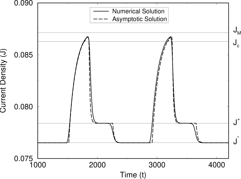
FIG. 5.:

REFERENCES

- [1] E-address bonilla@ing.uc3m.es. Fax: 34-1-6249445. Author to whom all correspondence should be addressed.
- [2] E-address pedroj@math.uc3m.es.
- [3] E-address herrero@sunma4.mat.ucm.es.
- [4] E-address kindelan@dulcinea.uc3m.es.
- [5] E-address velazque@sunma4.mat.ucm.es.
- [6] S. W. Teitsworth, R. M. Westervelt, and E. E. Haller, Phys. Rev. Lett. 51, 825 (1983).
- [7] A. M. Kahn, D. J. Mar, and R. M. Westervelt, Phys. Rev. B 43, 9740 (1991).
- [8] J. B. Gunn, IBM J. Res. Dev. 8, 141 (1964).
- [9] A. M. Kahn, D. J. Mar, and R. M. Westervelt, Phys. Rev. B 46, 7469 (1992).
- [10] A. M. Kahn, D. J. Mar, and R. M. Westervelt, Phys. Rev. B 45, 8342 (1992).
- [11] A. M. Kahn, D. J. Mar, and R. M. Westervelt, Phys. Rev. Lett. 46, 369 (1992).
- [12] S. W. Teitsworth and R. M. Westervelt, Phys. Rev. Lett. 53, 2587 (1984).
- [13] R. M. Westervelt and S. W. Teitsworth, J. Appl. Phys. 57, 5457 (1985).
- [14] L. L. Bonilla, Phys. Rev. B 45, 11642 (1992).
- [15] N. M. Haegel and A. M. White, Infrared Phys. 29, 915 (1989).
- [16] H. Kroemer, IEEE Trans. ED-15, 819 (1968).
- [17] L. L. Bonilla, I. R. Cantalapiedra, M. J. Bergmann, and S. W. Teitsworth, Semicond. Sci. Technol. 9, 599 (1994).
- [18] V. V. Mitin, Appl. Phys. A 39, 123 (1986).
- [19] E. Schöll, Solid-State Electron. 31, 539 (1988).
- [20] E. Schöll, Appl. Phys. A 48, 95 (1989).
- [21] T. Kuhn et al., Phys. Rev. B 48, 1478 (1993).
- [22] I. R. Cantalapiedra, L. L. Bonilla, M. J. Bergmann, and S. W. Teitsworth, Phys. Rev. B 48, 12278 (1993).
- [23] M. J. Bergmann, S. W. Teitsworth, L. L. Bonilla and I. R. Cantalapiedra, Phys. Rev. B 53, 1327 (1996).
- [24] S. W. Teitsworth, M. J. Bergmann, and L. L. Bonilla, in Nonlinear Dynamics and Pattern Formation in Semiconductors and Devices, Vol. 79 of Springer Proceedings in Physics, edited by F.-J. Niedernostheide (Springer-Verlag, Berlin-Heidelberg, 1995), pp. 46–69.
- [25] L. L. Bonilla and S. W. Teitsworth, Physica D 50, 545 (1991).
- [26] L. L. Bonilla, Physica D 55, 182 (1992).
- [27] D. Henry, Geometric theory of semilinear equations, Vol. 840 of Lecture Notes in Mathematics (Springer-Verlag, Berlin-Heidelberg, 1981).
- [28] L. L. Bonilla, F. J. Higuera, and S. Venakides, SIAM J. Appl. Math. 54, 1521 (1994).
- [29] F. J. Higuera, and L. L. Bonilla, Physica D 57, 161 (1992).
- [30] L. L. Bonilla and I. R. Cantalapiedra, Preprint, 1996.