Pattern Formation in a 2D Elastic Solid

Abstract

We present a dynamical theory of a two–dimensional martensitic transition in an elastic solid, connecting a high–temperature phase which is nondegenerate and has triangular symmetry, and a low–temperature phase which is triply degenerate and has oblique symmetry. A global mode–based Galerkin method is employed to integrate the deterministic equation of motion, the latter of which is derived by the variational principle from a nonlinear, nonlocal Ginzburg–Landau theory which includes the sound–wave viscosity. Our results display (i) the phenomenon of surface nucleation, and (ii) the dynamical selection of a length scale of the resultant patterns.

Dynamical pattern formation, while canonically associated with fluid systems such as convection cells, or initially fluid systems, such as is the case in eutectic solidification, also occurs in fully coherent solid–to–solid structural phase transformations which are purely elastic in character. Such phase transformations, generally known as “Martensites”, involve the formation of regions of the solid which become permanently strained relative to their undistorted parent phase, without the diffusive transport of matter, and without the introduction of crystallographic dislocations into the system.

A two–dimensional model of such a system is the principal topic of this paper and is described in more detail below, but it is worth nothing that considerable insight was gained into this problem by the study of conceptually straightforward one–dimensional models. The work of Bales and Gooding [1] dramatically illustrates the role of inertia in elastic systems with degenerate product states. This model included all of the important features of the potential energy which are present in the current study, and gave rise to a nontrivial, long–lived, patterned state. This early work did not examine the role of the boundaries of the system, but related work [2] using a single–product–state potential and again using inertial Hamiltonian dynamics demonstrated the role of the system boundary as a potential nucleating defect — in this system, a decaying subcritical excitation interacted with the free boundary to drive the system into the product state well. Because of the nature of the potential energy of this system (a nondegenerate product state), pattern formation was not possible. An extensive summary of the 1D work carried out by the Queen’s group can be found in Ref. [3].

In this paper we present a dynamical model of a $D>1$ martensitic transformation. We study the particular example of the transition undergone by a 2D elastic solid that is reminiscent of the 3D transition undergone by a real material. In 2D we let the high–temperature phase be nondegenerate and have triangular symmetry, and the low–temperature phase be triply degenerate and have oblique symmetry. This particular choice of parent and product phase symmetries leads to intriguing self–similar patterns, some of which we hoped to be able to access dynamically. The equation of motion is formulated using a variational continuum mechanics approach, and the elastic displacement field evolves in time under deterministic, inertial Hamiltonian dynamics. As the system evolves, it is forced to choose between the energetically equivalent minima, resulting in the formation of patterned states in which some of each possible product phase is present — we enforce the absence of dislocations by integrating the displacement field, not the components of the strain tensor, thus ensuring that the elastic compatibility relations are satisfied. The system is observed to begin the displacement from the free boundaries, consistent with the critical nucleus of the system existing at the surface, and the hydrodynamic selection of a characteristic length-scale for the resulting patterns is demonstrated.

The real material [4] that inspired our two–dimensional model system is lead orthovanadate, ${\rm Pb_{3}(VO_{4})_{2}}$, where a nested self–similar star–like patterned morphology occurs. We take as the plane of the model system the plane normal to the long axis of the trigonal unit cell in the physical system, and require that the potential energy reproduce the corresponding three–fold rotational symmetry. In ${\rm Pb_{3}(VO_{4})_{2}}$, the structural transformation changes the trigonal parent–phase unit cells to monoclinic product–phase cells, breaking the three–fold rotational symmetry along one of three equivalent directions. We model this by including three degenerate strain minima in a Ginzburg–Landau potential, the minima corresponding to area–preserving shear strains which locally stretch the system along one of three equivalent lines spaced $120^{\circ}$ apart. As in the one–dimensional systems, we include dissipation, inertia, and strain–gradient terms.

The dynamical variables of the model are the two components of the continuum vector displacement field, $u_{x}(x,y)$ and $u_{y}(x,y)$. Any value of the symmetric strain tensor for the system, derived from these displacements, can be expressed in terms of the three principal strains, which we label $e_{1}$, $e_{2}$, and $e_{3}$, where the $e_{1}$ strain corresponds to a uniform dilation of the system, and $e_{2}$ and $e_{3}$ correspond to the two area–preserving shear strains which stretch the system along one axis and contract it along the normal to this axis. The $e_{2}$ and $e_{3}$ strains are distinguished by having their stretch axes at $45^{\circ}$ to each other.

We implement a phenomenological free energy density which governs the dynamics as a temperature–dependent mechanical potential energy density. This free energy has several components: The local portion provides the essential nonlinearity of the system — it is this density, a function only of the principal strains, which respects the three–fold symmetry of the system and which gives rise to the symmetry–breaking degenerate stable minima. It is given by

$${\cal V}_{\rm local}={1\over 2}A{e_{1}}^{2}+{1\over 2}B({e_{2}}^{2}+{e_{3}}^{2})-{1\over 3}C({e_{2}}^{3}-3e_{2}{e_{3}}^{2})+{1\over 4}D({e_{2}}^{2}+{e_{3}}^{2})^{2}~{}.~{}$$ (1)

The parameters $A$ and $B$ are the linear elastic constants of the system, and vary with temperature. To this linear order, the potential is elastically isotropic. The parameters $C$ and $D$ reflect the nonlinearity of the system. The parameter $D$ must be positive for the potential to be globally stable, and the parameter $C$ governs the details of the potential wells. Changing the sign of $C$ changes the position of the global mimima in the $e_{2}$–$e_{3}$ plane, but not their overall structure.

Figure 1: Contour plot of the local potential energy, indicating the central metastable well and the three stable wells corresponding to strained states.

This potential is illustrated in Figure 1, which is a contour–plot of the $e_{2}$–$e_{3}$ portion of Eq. (1). The central metastable well is evident at the origin of the figure, where $e_{2}=e_{3}=0$, and the three globally stable product wells are evenly spaced at the same distance from the origin, at the linear combinations of $e_{2}$ and $e_{3}$ corresponding to stretching along the three $120^{\circ}$ lines. It is worth noting at this point that Fig. 1 is in the strain space of the system, and that the positions of the product–state wells in this space is not directly related to the orientation of the principal directions of expansion and compression for the corresponding strains.

In addition to the local terms, the correct description of the inertial dynamics requires that we also account for the kinetic energy of the system, the nonlocal or Ginzburg terms of the potential, and the dissipation. The Ginzburg terms prevent the system from forming unphysically small domains of the product state by breaking the scale–invariance of the linear system, and the dissipative terms provide for the removal of kinetic energy from the system as it goes from the initial state of high potential energy to the final, patterned state of low potential energy. The relevant kinetic, nonlocal, and dissipative terms are given by

$${\cal T} = {1\over 2}\rho({\dot{u}_{x}}^{2}+{\dot{u}_{y}}^{2})~{}~{},$$ (2)

$${\cal V}_{\rm nonlocal} = {1\over 2}g_{1}({e_{1,x}}^{2}+{e_{1,y}}^{2})+{1\over 2}g_{2}({e_{2,x}}^{2}+{e_{2,y}}^{2}+{e_{3,x}}^{2}+{e_{3,y}}^{2})~{}~{},$$ (3)

$${\rm and}\quad{\cal R} = {1\over 2}\gamma_{A}{\dot{e}_{1}}^{2}+{1\over 2}\gamma_{B}({\dot{e}_{2}}^{2}+{\dot{e}_{3}}^{2})~{}~{}.$$ (4)

All of the foregoing are intensive aspects of the system, independent of the details of the system geometry. The final ingredient in constructing the dynamics is to specify the system geometry. We choose a diamond–shaped system with two $120^{\circ}$ corners and two $60^{\circ}$ corners, as illustrated in the time–slices of Figures 2 $\rightarrow$ 4. The apparent stepped structure of the left–hand and right–hand edges is due to the shading algorithm. The model system has straight sides. The system geometry reflects a pragmatic compromise between the $120^{\circ}$ symmetry of the potential and the computational tractability of a square system, to which this geometry can be mapped for the purpose of performing the required numerical integrations.

The equation of motion for the dynamics of this system is the usual inertial Hamiltonian dynamics for the displacement field. The Lagrangian of the system is simply the integral of the Lagrangian density obtained by subtracting all of the potential–energy terms from the kinetic terms in the usual way. We have that

$$L=\int\!\int({\cal T}-{\cal V}_{\rm local}-{\cal V}_{\rm nonlocal})\cdot da~{}~{},$$ (5)

and the corresponding dissipation function is given by the area integral of the dissipation density,

$$R=\int\!\int{\cal R}\cdot da~{}~{}.$$ (6)

The Lagrangian and dissipation function so obtained contain the dynamical fields $u_{x}$ and $u_{y}$ through their contribution to the strains which appear in the potentials, as well as explicitly in the kinetic energy density. The equation of motion for the system is obtained by functional differentiation of the Lagrangian and dissipation function with respect to the dynamical fields and their time–derivatives, respectively, in the usual way [5]. Abstractly, we simply have that

$${\delta L\over\delta u}={\delta R\over\delta\dot{u}}~{}~{}.$$ (7)

Numerically, there are two approaches which suggest themselves at this point. The first of these is to obtain an analytic equation of motion for the system from Eq. (7), and then attempt to represent the dynamical fields and their derivatives either as an expansion in some set of basis functions, or on some kind of finite-element grid, and then deduce from the analytic equation of motion a corresponding equation of motion for the model degrees of freedom. This approach has the considerable advantage of conceptual straightforwardness, and was used with considerable success in the one–dimensional models previously cited. It is, however, complicated by the necessity of representing fourth derivatives of the displacement field, which occur as a result of the presence of the gradient terms, a complication which is rendered more difficult for the combinatorially large number of mixed partials which occur in the two–dimensional system.

For this reason, we chose to pursue a slightly different approach, which involves the construction not of an approximated equation of motion, but an approximated Lagrangian and dissipation function. The dynamical fields $u_{x}$ and $u_{y}$ are first expressed as expansions over a set of basis functions, in principle complete but of necessity truncated, and the new Lagrangian and dissipation function are constructed dependent on the amplitude coefficients and their time–derivatives. The solution to the system is then the equation of motion for the coefficient amplitudes. This is a globally–based modification of the familiar Galerkin method for solving partial differential equations.

Formally, the two methods are equivalent, but practically speaking, the latter method enjoys significantly better numerical stability, and a small advantage in the speed with which solutions are obtained, for a variety of reasons. In the latter method, the spatial integrations of the various densities need be computed only once, and lead to mode–coupling coefficients in the resulting mode–based Lagrangian. The integrations involve products of lower–order derivatives of the displacement fields, and in addition to the greater numerical stability of this process, also lends itself to the exact computation of the mode–coupling coefficients. There need be no other approximations in the system other than the necessary truncation of the set of modes used to represent the displacement fields. A complete discussion of this technique will be given in a later publication.

The results of one particular dynamical run, illustrative of all of the major effects observed in this study, are presented in Figures 2 $\rightarrow$ 4. Each panel of each figure is a snapshot of the $e_{2}$–$e_{3}$ strain state of the system. The panels of the first two figures, Figs. 2 and 3, are evenly spaced in time and cover the early portion of the dynamics through to approximately three times the speed–of–sound travel time across the long axis of the fully–transformed system. The final figure, Fig. 4, consists of snapshots spaced at eight times the interval of the first two figures, and shows the late stage of the dynamics. In all of these figures, regions in which a given stable strain state is approximately fully developed are indicated by the grey zones in these figures. The accompanying arrows indicate the direction in which the region is stretched, although it should be kept in mind that the minima correspond to area–preserving shear strains with a corresponding contraction at $90^{\circ}$ to the expansion direction. The black regions of these figures correspond to portions of the system which are close to the parent phase, with approximately zero strain.

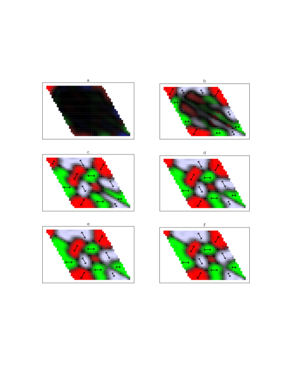
Figure 2: Time–slices of the $e_{2}$–$e_{3}$ state of the dynamical system. The shaded grey regions in each panel are regions of the system which have achieved different stable transformation strains, the precise orientation being indicated by the accompanying arrows. This figure shows a sequence of snapshots of the system during the earliest stages of the transformation, during which transformed domains initially form around the boundaries of the system, followed by the formation of interior domains of approximately uniform size with complementary strain orientations.

We present one particular study undertaken using the mode–based dynamical technique described previously. In order to expedite the dynamics, this study was undertaken with the linear restoring force for shear, coefficient $B$ of Eq. (1), strongly negative. We began with low–amplitude random initial condition for the initial displacements, and with the initial velocities set to zero, and proceeded under deterministic inertial dynamics with free boundary conditions.

The precise parameter values were chosen to be $A=0.0$, $B=-2000$, $C=16547.7$, $D=118331.0$, $\gamma_{A}=0.1$, $\gamma_{B}=6.0$, and $g_{1}=1.2$, and $g_{2}=4.0$. This parameter set gave product–state well depths of order one, in the arbitrary but self–consistent energy units defined by the potentials, and strain amplitudes for the well bottoms of $0.1$.

As indicated in Fig. 2, the system begins the transformation from the boundaries, first falling in to the stable minima at the corners, then subsequently along the edges, and then forming a patchwork of domains throughout the system. Given the absence of linear restoring forces for the shear strains, it is noteworthy that this initial development stage for product states does not take place immediately. Local potential energy considerations would suggest that the behaviour should be that of spinodal decomposition. In this system, however, there are two additional complementary effects, those of inertia and elastic accommodation, which prevent the system from spontaneously transforming itself entirely into the product–phase, and both of these effects account for why the transformation begins at the surface.

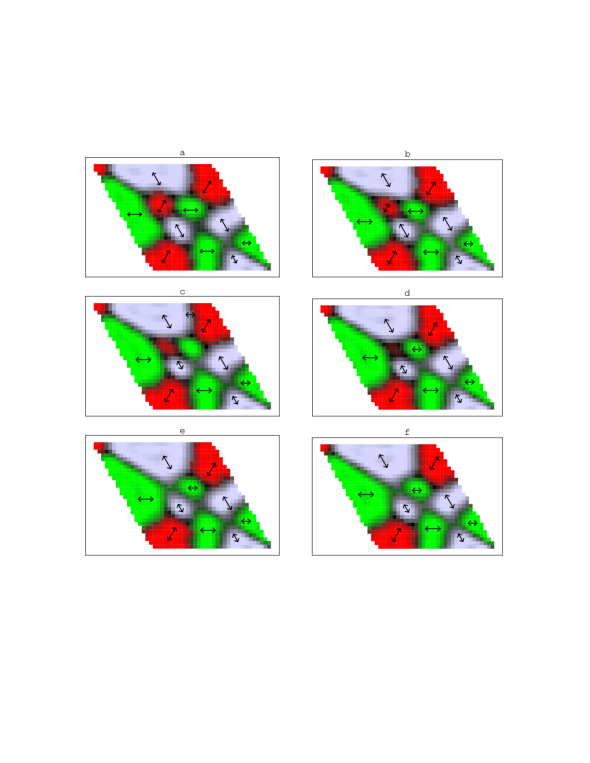
Figure 3: Late–stage snapshots of the dynamical system. This figure is a continuation of Fig. 3, but with the panels separated by a time interval eight times larger than that of Figs. 2 and 3. The two complementarily–oriented domains in the upper left portion of the figure expand and push the smaller domains off the right–hand end, until finally the system consists of an arbitrarily long–lived twinned state, higher in energy than the system’s ground state.

Elastic accommodation provides a penalty, in terms of elastic energy, for forming an isolated region of product–phase in the centre of the system. In order to maintain the elastic coherency of the system, such a structure must be surrounded by a displacement field which relaxes towards the unstrained parent phase at distances large compared to the size of the structure. This accommodation effect is one of the principal differences between elastic hydrodynamics and the more conventional convective hydrodynamics, which, even in the inertial regime, is not subject to an analogous coherency constraint.

The accommodation constraint leaves open the possibility that the system may suddenly form a system–wide network of self–accommodating domains. Such a structure would certainly rapidly minimize the potential energy of the system, but in this case it is the inertia of the system which prevents it from following such a dynamical path. In order to collectively move all the parts of the system in the required co-ordinated manner would require a substantial amount of kinetic energy. The energy required to support the required velocity field is simply not available, and so we see instead that for both of these reasons, the dynamics begin around the edges and the corners, where the accommodation constraint can be avoided entirely and the inertia of the portion of the system near the tip of one of the points is small.

Following the initial “nucleation” (though we use this word with some caution) stage of the dynamics, the system forms an interior patchwork of transformed domains of approximately uniform size, about which we shall have more to say in a moment. The system then undergoes a coarsening process during which large domains tend to become larger, and smaller domains are absorbed into larger domains or are expelled from the system, illustrated in Figs. 2 and 3. The strain order parameter is not conserved, but large domains tend to grow at the expense of smaller adjacent domains, and because of the inertial and accommodation effects, these adjacent domains tend to consist of complementary product phase. Thus the dynamics give the appearance of the order parameter being, in some sense, approximately conserved during this intermediate phase.

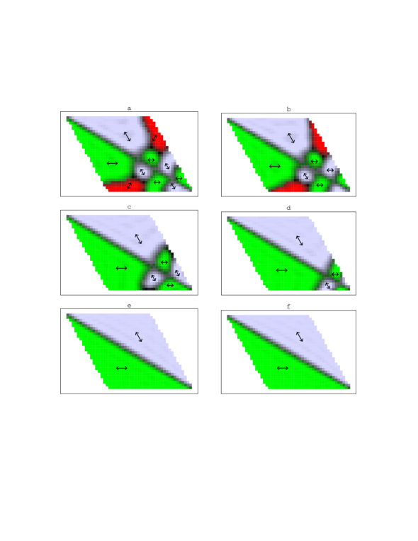
Figure 4: Continuation of the series of snapshots from Fig. 2, with the same spacing in time. These panels show the coarsening of the system at intermediate times in the dynamics, during which the smaller domains shrink and are removed from the system while the larger domains begin to domiante the system. This figure also shows the reflection symmetry of the domain orientations, present in the initial condition, to good advantage.

The phenomenon in which the initial patchwork of domains all have approximately the same size scale is not universal behaviour for the system, but rather is understood to be a consequence of the interaction between the inertial dynamics and the damping of the system. The length–scale can in fact be quantitatively predicted from a simple linear instability analysis [6]. We consider a travelling shear–wave displacement field of the form

$$u_{x}=\alpha e^{i(k\cdot y-\omega t)},~{}~{}~{}~{}~{}~{}~{}~{}~{}u_{y}=0,$$ (8)

for some amplitude $\alpha$. Substituting this into the linear part of the Lagrangian, Eq. (5), and into the dissipation function, Eq. (6), we find that the resulting equation of motion gives the frequency of the shear wave as a function of its wavenumber. The linear growth rate is the imaginary part of the frequency, and is given by

$${\rm Im}(\omega)={-\gamma_{B}\over 4\rho}k^{2}+\left[{|B|\over 8\rho}k^{2}-\left({g_{2}\over 8\rho}-{\gamma_{B}^{2}\over 16\rho^{2}}\right)k^{4}\right]^{1\over 2},$$ (9)

where we have chosen the most positive of the possible roots of a quadratic relation in $\omega$. The values chosen for $\gamma_{B}$ and $g_{2}$ simplify the situation somewhat by making the square root in Eq. (9) purely imaginary. The wavenumber with the maximum growth rate is obtained by maximizing the above relation with respect to $k$, and we have

$$k^{2}_{\rm growth}=\left(|B|\over{2g_{2}+4\gamma_{B}\sqrt{g_{2}\over 8\rho}}\right).$$ (10)

Substituting the parameter values used for our dynamical study, we find that the length scale for the maximum growth rate is $l=0.7$, or approximately one–third of the length of one of the sides of the diamond, and that the earliest fully–transformed picture of the system supports the contention that a dynamically–selected length scale of this magnitude dominates the morphology of the early–stage dynamics. This conclusion is further supported by another run, not illustrated here [7], for which the parameter $B$ was set equal to zero, and a variety of lengths scales were observed in the initially developed strain pattern.

The late stage of the dynamics, indicated in Fig. 4, illustrates the importance of the reflection symmetry of the initial displacement field across the long axis of the system. This is a symmetry which is preserved under the dynamics of the system, and which therefore persists into the final state. The only possible homogeneously strained minimum, and therefore the lowest possible energy state for this system, is that in which the system is stretched along the short axis. The dynamics do not access this minimum, however, and instead reaches a final state which consists of two domains, consistent with the symmetry of the initial conditions, and separated by a domain wall. This patterned state is expected to be arbitrarily long–lived under our deterministic dynamics, although it is far from the lowest possible energy of the system.

The model presented here incorporates several of the essential features of diffusionless structural phase transformations which are known to give rise to pattern formation in a variety of solid systems. We have abstracted the essential features of such systems — symmetry, inertia, and dissipation — which are sufficient to give rise to the pattern–forming dynamics which are ubiquitous in a large variety of natural systems [8], while leaving out the precise crystallographic details which vary between such systems and which dominate them at much shorter length scales than those of interest here. Our abstract system is also not fully three–dimensional, as are all real coherent nonlinear elastic systems, but this is evidently not a requirement.

With only these essential features, and guided by the suggestive results of the one–dimensional work, we have observed pattern–formation dynamics, including one instance of an arbitrarily long–lived pattern.

We acknowledge helpful comments of Nick Schryvers and Bob Kohn. This work was supported by the NSERC of Canada.

References

- [1] G. S. Bales and R. J. Gooding, Phys. Rev. Lett. 67, 3412 (1991).
- [2] A. C. E. Reid and R. J. Gooding, Phys. Rev. B 50, 3588 (1994).
- [3] B. P. van Zyl and R. J. Gooding, Met. & Mat. Trans. A 27, 1203 (1996).
- [4] C. Manolikas and S. Amelinckx, Phys. Stat. Solidi (a) 60, 607 (1980); ibid, 61, 179 (1980).
- [5] L. D. Landau and E. M. Lifshitz, Statistical Physics, 3rd ed. Part 1(Pergamon, Oxford, 1980).
- [6] M. C. Cross and and P. C. Hohenberg, Rev. Mod. Phys. 65, 851 (1993).
- [7] A. C. E. Reid, Ph. D. Thesis, Queen’s University, Sept. 1994.
- [8] G. B. Olson and M. Cohen, Proc. ICOMAT 79, Massachusetts Institute of Technology, 1979, p. 310.