Persistence exponents for fluctuating interfaces

Abstract

Numerical and analytic results for the exponent $\theta$ describing the decay of the first return probability of an interface to its initial height are obtained for a large class of linear Langevin equations. The models are parametrized by the dynamic roughness exponent $\beta$, with $0<\beta<1$; for $\beta=1/2$ the time evolution is Markovian. Using simulations of solid-on-solid models, of the discretized continuum equations as well as of the associated zero-dimensional stationary Gaussian process, we address two problems: The return of an initially flat interface, and the return to an initial state with fully developed steady state roughness. The two problems are shown to be governed by different exponents. For the steady state case we point out the equivalence to fractional Brownian motion, which has a return exponent $\theta_{S}=1-\beta$. The exponent $\theta_{0}$ for the flat initial condition appears to be nontrivial. We prove that $\theta_{0}\to\infty$ for $\beta\to 0$, $\theta_{0}\geq\theta_{S}$ for $\beta<1/2$ and $\theta_{0}\leq\theta_{S}$ for $\beta>1/2$, and calculate $\theta_{0,S}$ perturbatively to first order in an expansion around the Markovian case $\beta=1/2$. Using the exact result $\theta_{S}=1-\beta$, accurate upper and lower bounds on $\theta_{0}$ can be derived which show, in particular, that $\theta_{0}\geq(1-\beta)^{2}/\beta$ for small $\beta$.

I Introduction

The statistics of first passage events for non-Markovian stochastic processes has attracted considerable recent interest in the physical literature. Such problems appear naturally in spatially extended nonequilibrium systems, where the dynamics at a given point in space becomes non-Markovian due to the coupling to the neighbours. The asymptotic decay of first passage probabilities turns out to be hard to compute even for very simple systems such as the one-dimensional Glauber model [1] or the linear diffusion equation with random initial conditions [2]. Indeed, determining the first passage probability of a general Gaussian process with known autocorrelation function is a classic unsolved problem in probability theory [3, 4, 5].

In this paper we address the first passage statistics of fluctuating interfaces. The large scale behaviour of the models of interest is described by the linear Langevin equation

$$\frac{\partial h}{\partial t}=-(-\nabla^{2})^{z/2}h+\eta$$ (1)

for the height field $h(x,t)$. Here the dynamic exponent $z$ (usually $z=2$ or 4) characterizes the relaxation mechanism, while $\eta(x,t)$ is a Gaussian noise term, possibly with spatial correlations. We will generally assume a flat initial interface, $h(x,0)=0$. Since (1) is linear, $h(x,t)$ is Gaussian and its temporal statistics at an arbitrary fixed point in space is fully specified by the autocorrelation function computed from (1),

$$A(t,t^{\prime})\equiv\langle h(x,t)h(x,t^{\prime})\rangle=K[(t^{\prime}+t)^{2\beta}-|t^{\prime}-t|^{2\beta}],$$ (2)

where $K$ is some positive constant, and $\beta$ denotes the dynamic roughness exponent, which depends on $z$ and on the type of noise considered. For example, for uncorrelated white noise $\beta=(1/2)[1-d/z]$ for a $d$-dimensional interface, while for volume conserving noise $\beta=(1/2)[1-(d+2)/z]$ [6]. An interface is rough if $\beta>0$. In the present work we regard $\beta$ as a continuous parameter in the interval $]0,1[$. Note that for $\beta=1/2$ eq.(2) reduces to the autocorrelation function of a random walk, corresponding to the limit $z\to\infty$ (no relaxation) of eq.(1) with uncorrelated white noise.

To define the first passage problems of interest, consider the quantity

$$P(t_{0},t)={\rm Prob}[h(x,s)\neq h(x,t_{0})\;\;\forall s:t_{0}<s<t_{0}+t].$$ (3)

We focus on two limiting cases. For $t_{0}=0$, $P(t_{0},t)$ reduces to the probability $p_{0}(t)$ that the interface has not returned to its initial height $h=0$ at time $t$. This will be referred to as the transient persistence probability, characterized by the exponent $\theta_{0}$,

$$p_{0}(t)\equiv P(0,t)\sim t^{-\theta_{0}},\;\;\;t\to\infty.$$ (4)

On the other hand, for $t_{0}\to\infty$ the interface develops roughness on all scales and the memory of the flat initial condition is lost. In this limit $P(t_{0},t)$ describes the return to a rough initial configuration drawn from the steady state distribution of the process, and the corresponding steady state persistence probability $p_{S}(t)$ decays with a distinct exponent $\theta_{S}$,

$$p_{S}(t)\equiv\lim_{t_{0}\to\infty}P(t_{0},t)\sim t^{-\theta_{S}},\;\;\;t\to\infty.$$ (5)

In general, one expects that $P(t_{0},t)\sim t^{-\theta_{S}}$ for $t\ll t_{0}$ and $P(t_{0},t)\sim t^{-\theta_{0}}$ for $t\gg t_{0}$, with a crossover function connecting the two regimes.

A particular case of the steady state persistence problem was studied previously in the context of tracer diffusion on surfaces [7]. In this work it was observed that the distribution of first return times has a natural interpretation as a distribution of trapping times during which a diffusing particle is buried and cannot move; thus the first passage exponent may translate into an anomalous diffusion law. A simple scaling argument (to be recalled below in Section V) was used to derive the relation

$$\theta_{S}=1-\beta,$$ (6)

which was well supported by numerical simulations for $\beta=1/8$. A primary motivation of the present work is therefore to investigate the validity of this relation through simulations for other values of $\beta$ and refined analytic considerations, as well as to understand why it fails for the transient persistence exponent $\theta_{0}$.

The paper is organized as follows. In the next section we convert the non-stationary stochastic process $h(x,t)$ into a stationary Gaussian process in logarithmic time [2, 5]. This representation will provide us with a number of bounds and scaling relations, and will be used in the simulations of Section IV.C. A perturbative calculation of the persistence exponents in the vicinity of $\beta=1/2$ is presented in Section III. The simulation results are summarized in Section IV. Section V reviews the analytic basis of the relation (6) and makes contact to earlier work on the return statistics of fractional Brownian motion, while Section VI employs the expression (6) for $\theta_{S}$ to numerically generate exact upper and lower bounds on $\theta_{0}$. Finally, some conclusions are offered in Section VII.

II Mapping to a stationary process

Following Refs.[2, 5] we introduce the normalized random variable $X=h/\sqrt{\langle h^{2}\rangle}$ which is considered a function of the logarithmic time $T=\ln t$. The Gaussian process $X(T)$ is then stationary by construction, $\langle X(T)X(T^{\prime})\rangle=f_{0}(T-T^{\prime})$, and the autocorrelation function $f_{0}$ obtained from (2) is

$$f_{0}(T)=\cosh(T/2)^{2\beta}-|\sinh(T/2)|^{2\beta}.$$ (7)

In logarithmic time the power law decay (4) of the persistence probability becomes exponential, $p_{0}(T)\sim\exp(-\theta_{0}T)$, and the task is to determine the decay rate $\theta_{0}$ as a functional of the correlator $f_{0}$ [3, 4, 5].

Similarly a normalized stationary process can be associated with the steady state problem. First define the height difference variable

$$H(x,t;t_{0})\equiv h(x,t+t_{0})-h(x,t_{0})$$ (8)

and compute its autocorrelation function in the limit $t_{0}\to\infty$,

$$A_{S}(t,t^{\prime}) = \lim_{t_{0}\to\infty}\langle H(x,t;t_{0})H(x,t^{\prime};t_{0})\rangle$$ (9)

$$= \lim_{t_{0}\to\infty}[A(t_{0}+t,t_{0}+t^{\prime})-A(t_{0}+t,t_{0})$$ (12)

$$\phantom{\lim_{t_{0}\to\infty}[}-A(t_{0},t_{0}+t^{\prime})+A(t_{0},t_{0})]$$

$$=K[t^{2\beta}+t^{\prime 2\beta}-|t^{\prime}-t|^{2\beta}],$$

which is precisely the correlator of fractional Brownian motion with Hurst exponent $\beta$ [8] (see Section V). Next $A_{S}(t,t^{\prime})$ is normalized by $\sqrt{A_{S}(t,t)A_{S}(t^{\prime},t^{\prime})}$ and rewritten in terms of $T=\ln t$. This yields the autocorrelation function

$$f_{S}(T)=\cosh(\beta T)-\frac{1}{2}|2\sinh(T/2)|^{2\beta}.$$ (13)

Comparison of eqs.(7) and (13) makes it plausible that the two processes have different decay rates of their persistence probabilities. Both functions have the same type of short time singularity

$$f_{0,S}(T)=1-{\cal O}(|T|^{2\beta}),\;\;\;T\to 0,$$ (14)

which places them in the class $\alpha=2\beta$ in the sense of Slepian [3]. However, for large $T$ they decay with different rates, $f_{0,S}(T)\sim\exp(-\lambda_{0,S}T)$ for $T\to\infty$, where

$$\lambda_{0}=1-\beta,\;\;\;\lambda_{S}=\min[\beta,1-\beta]$$ (15)

can be interpreted, in analogy with phase ordering kinetics, as the autocorrelation exponents [9] of the two processes.

For a stationary Gaussian process with a general autocorrelator $f(T)$, the calculation of the decay exponent $\theta$ of the persistence probability is very hard. Only in a very few cases exact results are known [3]. Approximate results can be derived for certain classes of autocorrelators $f(T)$. For example, when $f(T)=1-O(T^{2})$ for small $T$ (an example being the linear diffusion equation [2]), the density of zero crossings is finite and an independent interval approximation (IIA) [2] gives a very good estimate of $\theta$. However, for any other process for which $f(T)=1-O(|T|^{\alpha})$ for small $T$ with $\alpha<2$, the density of zeros is infinite and the IIA breaks down. For general proceses with $\alpha=1$, a perturbative method (when the process is not far from Markovian) and an approximate variational method was developed recently [5]. This method will be applied to the present problem in Section III. In the remainder of this section we collect some exact bounds on $\theta$; further bounds will be derived in Section VI.

Slepian [3] has proved the following useful theorem for stationary Gaussian processes with unit variance: For two processes with correlators $f_{1}(T)$ and $f_{2}(T)$ such that $f_{1}(T)\geq f_{2}(T)\geq 0$ for all $T$, the corresponding persistence probabilities satisfy $p_{1}(T)\geq p_{2}(T)$; in particular, the inequality $\theta_{1}\leq\theta_{2}$ holds for the asymptotic decay rates. By applying this result to the correlators (7) and (13) we can generate a number of relations involving the return exponents $\theta_{0}$ and $\theta_{S}$. For example, taking the derivative of (7) with respect to $\beta$ one discovers that $f_{0}(T)$ increases monotonically with decreasing $\beta$ for all $T$, and consequently

$$\theta_{0}(\beta)\geq\theta_{0}(\beta^{\prime})\;\;\;{\rm if}\;\;\beta\leq\beta^{\prime}.$$ (16)

For $\beta\leq\beta^{\prime}\leq(2\ln 2)^{-1}$ the stronger inequality

$$(1-\beta^{\prime})\theta_{0}(\beta)\geq(1-\beta)\theta_{0}(\beta^{\prime})$$ (17)

is proved in the Appendix.

Moreover, rewriting (13) in the form

$$f_{S}(T)=e^{-\beta|T|}+\frac{1}{2}e^{\beta|T|}[1-e^{-2\beta|T|}-(1-e^{-|T|})^{2\beta}]$$ (18)

it is evident that $f_{S}(T)<\exp(-\beta|T|)$ for $\beta<1/2$ and $f_{S}(T)>\exp(-\beta|T|)$ for $\beta>1/2$. A process characterized by a purely exponential autocorrelation function $\exp(-\lambda|T|)$ is Markovian, and its persistence probability can be computed explicitly [3]; the asymptotic decay rate $\theta$ is equal to the decay rate $\lambda$ of the correlation function. Thus the fact that $f_{S}(T)$ can be bounded by Markovian (exponential) correlation functions supplies us with the inequalities

$$\theta_{S}\geq\beta,\;\;\;\beta<1/2$$

$$\theta_{S}\leq\beta,\;\;\;\beta>1/2.$$ (19)

The last inequality can be sharpened to

$$\theta_{S}\leq 1/2,\;\;\;\beta>1/2.$$ (20)

This will be demonstrated in the Appendix, where we also prove that

$$\theta_{0}\geq 1-\beta\;\;{\rm for}\;\;\beta<1/2$$

$$\theta_{0}\leq 1-\beta\;\;{\rm for}\;\;\beta>1/2$$ (21)

and

$$\theta_{0}\geq\theta_{S}\;\;{\rm for}\;\;\beta<1/2$$

$$\theta_{0}\leq\theta_{S}\;\;{\rm for}\;\;\beta>1/2.$$ (22)

Next we record some relations for special values of $\beta$. We noted already that for $\beta=1/2$ the interface fluctuations reduce to a random walk, corresponding to the Markovian correlator $f_{0}(T)=f_{S}(T)=\exp(-|T|/2)$, for which $\theta=\lambda=1/2$ [3]. Hence

$$\theta_{0}(1/2)=\theta_{S}(1/2)=1/2.$$ (23)

For $\beta=1$ both (7) and (13) become constants, $f_{0}(T)\equiv f_{S}(T)\equiv 1$. This implies that the corresponding Gaussian process is time-independent, and consequently

$$\lim_{\beta\to 1}\theta_{0}(\beta)=\lim_{\beta\to 1}\theta_{S}(\beta)=0.$$ (24)

For $\beta\to 0$ the transient correlator (7) degenerates to the discontinuous function $f_{0}(0)=1$, $f_{0}(T>0)=0$. Since this is bounded from above by the Markovian correlator $f(T)=e^{-\lambda|T|}$ for any $\lambda$, we conclude that

$$\lim_{\beta\to 0}\theta_{0}(\beta)=\infty.$$ (25)

In contrast, the steady state correlator tends to a nonzero constant, $\lim_{\beta\to 0}f_{S}(T)=1/2$ for $T>0$, with a discontinuity at $T=0$, and therefore $\theta_{S}$ is expected to remain finite for $\beta\to 0$. Note that all the relations derived for $\theta_{S}$ – equations (19,20,24) – are consistent with $\theta_{S}=1-\beta$.

III Perturbation theory near $\beta=1/2$

We have already remarked that both the steady state and the transient processes reduce to a Markov process when $\beta=1/2$. Two of us have developed a perturbation theory for the persistence exponent of a stationary Gaussian process whose correlation function is close to a Markov process [5]. When the persistence probability for a Markov process is written in the form of a path integral, it is found to be related to the partition function of a quantum harmonic oscillator with a hard wall at the origin. The persistence probability for a process whose correlation function differs perturbatively from the Markov process, i.e. whose autocorrelation function is

$$f(T)=\exp\left(-\lambda|T|\right)+\epsilon\phi(T),$$ (26)

may then be calculated from a knowledge of the eigenstates of the quantum harmonic oscillator. In (26) we have used the same normalization, $f(0)=1$, as elsewhere in this paper. With this normalization, $\phi(0)=0$. (Note that a different normalization was employed in ref. [5].)

If $\beta=1/2+\epsilon$, equations (7) and (13) may be written in the form

$$f_{0,S}=\exp\left(-{|T|\over 2}\right)+\epsilon\phi_{0,S}(|T|)+{\cal O}(\epsilon^{2}),$$ (27)

where

$$\phi_{0} = 2\cosh{T\over 2}\ln\left(\cosh{T\over 2}\right)-2\sinh{T\over 2}\ln\left(\sinh{T\over 2}\right),$$ (28)

$$\phi_{S} = \sinh{T\over 2}\left(T-2\ln\left(2\sinh{T\over 2}\right)\right).$$ (29)

The result for the persistence exponent (equivalent to equation (7) of reference [5]) may most conveniently be written in the form [11]

$$\theta=\lambda\left\{1-\epsilon{2\lambda\over\pi}\int_{0}^{\infty}\phi(T)\left[1-\exp(-2\lambda T)\right]^{-3/2}dT\right\}.$$ (30)

Substituting (28) and (29) into (30), one finds (after some algebra)

$$\theta_{0} = {1\over 2}-\epsilon(2\sqrt{2}-1)+{\cal O}(\epsilon^{2}),$$ (31)

$$\theta_{S} = {1\over 2}-\epsilon+{\cal O}(\epsilon^{2}).$$ (32)

Eqn. (32) agrees with the relation $\theta_{S}=1-\beta$, while (31) compares favourably with the stationary Gaussian process simulations for $\beta=0.45$ and $\beta=0.55$ to be presented in Section IV.C.

IV Simulation results

A Solid-on-solid models

Simulations of one-dimensional, discrete solid-on-solid models were carried out for $\beta=1/8$, $\beta=1/4$ and $\beta=3/8$. The case $\beta=1/8$ describes an equilibrium surface which relaxes through surface diffusion, corresponding to $z=4$ in (1) and volume conserving noise with correlator

$$\langle\eta(x,t)\eta(x^{\prime},t^{\prime})\rangle=-\nabla^{2}\delta(x-x^{\prime})\delta(t-t^{\prime}).$$ (33)

The cases $\beta=1/4$ and $\beta=3/8$ are realized for nonconserved white noise in (1) and dynamic exponents $z=2$ and $z=4$, respectively [6].

In all models the interface configuration is described by a set of integer height variables $h_{i}$ defined on a one-dimensional lattice $i=1,...,L$ with periodic boundary conditions. For simulations of the transient return problem, large lattices ($L=2\times 10^{5}$ – $2\times 10^{6}$) were used, while for the steady state problem we chose small sizes, $L=100-200$ for dynamic exponent $z=4$ and $L=1000$ for $z=2$, in order to be able to reach the steady state within the simulation time.

The precise simulation procedure is somewhat dependent on whether the volume enclosed by the interface is conserved (as for $\beta=1/8$) or not. To simulate the transient return problem with conserved dynamics, the interface was prepared in the initial state $h_{i}=0$, and each site was equipped with a counter that recorded whether the height $h_{i}$ had returned to $h_{i}=0$. The fraction of counters still in their initial state then gives the persistence probability $p_{0}(t)$. For the steady state problem the interface was first equilibrated for a time $t_{\rm eq}$ large compared to the relaxation time $\sim L^{z}$ [6, 12]. Then the configuration $h_{i}(t_{\rm eq})$ was saved, and the fraction of sites which had not yet returned to $h_{i}(t_{\rm eq})$ was recorded over a prescribed time interval $t_{\rm eq}<t<t_{\rm eq}+t_{1}$. At the end of that interval the current configuration $h_{i}(t_{\rm eq}+t_{1})$ was chosen as the new initial condition, and the procedure was repeated. After a suitable number of repetitions (typically $10^{4}$ for $z=4$, and 2000 for $z=2$), the surviving fraction gives an estimate of $p_{S}$.

The models used in the cases $\beta=1/4$ and $\beta=3/8$ are growth models, in which an elementary step consists in chosing at random a site $i$ and then placing a new particle, $h_{j}\to h_{j}+1$, either at $j=i$ or at one of the two nearest neighbour sites $j=i\pm 1$, depending on the local environment. For these nonconserved models the procedures described above have to be modified such that the calculation of the surviving fractions $p_{0}$ and $p_{S}$ is performed only when a whole monolayer – that is, one particle per site – has been deposited. At these instances the average height is an integer which can be subtracted from the whole configuration in order to decide whether a given height variable has returned to its initial state when viewed in a frame moving with the average growth rate.

We now briefly describe the results obtained in the conserved case. In [7] the steady state return problem for $\beta=1/8$ was investigated in the framework of the standard one-dimensional solid-on-solid model with Hamiltonian

$${\cal H}=J\sum_{i}|h_{i+1}-h_{i}|$$ (34)

and Arrhenius-type surface diffusion dynamics [13]. We have extended these simulations to longer times and to different values of the coupling constant $J$. Figure 1 shows that the exponent $\theta_{S}$ is independent of $J$, and that its value is numerically indistinguishable from $\theta_{S}=7/8$ predicted by (6).

Since the transient persistence probability $p_{0}$ decays very rapidly for $\beta=1/8$, a more efficient model was needed in order to obtain reasonable statistics. We therefore used a restricted solid-on-solid (RSOS) model introduced by Rácz et al. [14]. In this model the nearest neighbour height differences are restricted to

$$|h_{i+1}-h_{i}|\leq 2.$$ (35)

In one simulation step a site $i$ is chosen at random, and a diffusion move to a randomly chosen neighbour is attempted. If the attempt fails due to the condition (35), a new random site is picked. Figure 2 shows the transient persistence probability $p_{0}(t)$ obtained from a large scale simulation of this model. The curve still shows considerable curvature, and we are only able to conclude that probably $\theta_{0}>3.3$ for this process.

FIG. 1.: Steady state persistence probability $p_{S}(t)$ for the Arrhenius surface diffusion model with coupling constant $J=0.25$, 0.5 and 1. Systems of size $L=100$ were equilibrated for $t_{\rm eq}=5\times 10^{7}$ attempted moves per site. Then data were collected over $10^{4}$ time intervals of length $t_{1}=10^{4}$. The dashed line has slope $\theta_{S}=1-\beta=7/8$.

FIG. 2.: Transient persistence probability $p_{0}(t)$ for three different solid-on-solid models described in the text. The system sizes used were $L=2\times 10^{5}$ for $\beta=1/8$, and $L=2\times 10^{6}$ for $\beta=1/4$ and $\beta=3/8$. For $\beta=1/8$ ($\beta=1/4$) an average over 1000 (10) runs was taken, while the data for $\beta=3/8$ constitute a single run. The slopes of the dashed lines correspond to the exponent estimates in the fourth column of Table I.

Figure 2 also shows transient results for $\beta=1/4$ and $\beta=3/8$. In the former case we used a growth model introduced by Family [15], in which the deposited particle is always placed at the lowest among the chosen site $i$ and its neighbours, whereas for $\beta=3/8$ we used the curvature model introduced in [16]. Our best estimates of $\theta_{0}$ for these models are collected in Table I, along with the values for $\theta_{S}$ which agree, within numerical uncertainties, with the relation (6) in all cases.

B Discretized Langevin equations

We solved equation (1) in discretized time and space for the real valued function $h(x_{i},t_{n})$, where $t_{n}\equiv n\Delta t$ and $x_{i}\equiv i\Delta x$ with $n=0,1,2,\dots$ and $i=0,\dots,L-1$ in a system with periodic boundary conditions.

For the time discretization we used a simple forward Euler differencing scheme [17]:

$$\frac{\partial h(x_{i},t_{n})}{\partial t}\equiv\frac{h(x_{i},t_{n+1})-h(x_{i},t_{n})}{\Delta t}.$$ (36)

The spatial derivatives for the cases $z=2$ and $z=4$ considered in the simulations were discretized as

$$\nabla^{2}h(x_{i}) \equiv h(x_{i-1})-2h(x_{i})+h(x_{i+1}),$$ (37)

$$(\nabla^{2})^{2}h(x_{i}) \equiv h(x_{i-2})-4h(x_{i-1})+6h(x_{i})$$ (39)

$$-4h(x_{i+1})+h(x_{i+2})$$

for the function $h(x_{i})\equiv h(x_{i},t_{n})$ at any given time $t_{n}$. Here and in the simulations, the spatial lattice constant $\Delta x$ was set to unity.

With these definitions, we iterated the equation

$$h(x_{i},t_{n+1}) = h(x_{i},t_{n})-\Delta t(-\nabla^{2})^{z/2}h(x_{i},t_{n})$$ (41)

$$\phantom{h(x_{i},t_{n})}+\sigma\sqrt{\Delta t}\eta(x_{i},t_{n})$$

where $\eta(x_{i},t_{n})$ is a Gaussian distributed random number with zero mean and unit variance whose correlations will be specified below.

Von Neumann stability analysis [17] shows that values $\Delta t\leq 1/2$ and 1/8 for $z=$ 2 and 4, respectively, have to be used to keep the noise–free iteration stable. The simulations showed that the scheme remained stable with $\Delta t=0.4$ and 0.1 even in the noisy case.

FIG. 3.: (a) Steady state persistence probability $p_{S}(t)$ from the numerical solution of the discretized Langevin equation with $z=2$ and correlated noise ($\rho=-0.1,0.1,0.3$). The thick lines represent fits to the last decade of $p_{S}(t)$. The slopes are given in the second column of Table I. (b) Same as (a) for the transient persistence probability $p_{0}(t)$.

We used white noise $\eta_{w}(x_{i},t_{n})$ with a correlator

$$\langle\eta_{w}(x_{i},t_{n})\eta_{w}(x_{j},t_{m})\rangle=\delta_{i,j}\delta_{n,m}$$ (42)

in the simulations, as well as spatially correlated noise $\eta_{\rho}(x_{i},t_{n})$ with

$$\langle\eta_{\rho}(x_{i},t_{n})\eta_{\rho}(x_{j},t_{m})\rangle=\sigma^{2}g_{\rho}(x_{i}-x_{j})\delta_{n,m}$$ (43)

where

$$g_{\rho}(x_{i}-x_{j})\equiv\left\{\begin{array}[]{rl}|x_{i}-x_{j}|^{2\rho-1}&,i\neq j\\ 1&,i=j\end{array}\right.$$ (44)

and $\rho<1/2$ a real number. A different choice of regularizing $g(0)$ [18] did not change the results. If $S_{\rho}(k)$ denotes the discrete Fourier transform of $g_{\rho}$, we defined

$$\eta_{\rho}(k,t)\equiv\sqrt{|S_{\rho}(k)|}r_{k}\exp(2\pi i\varphi_{k})$$ (45)

with $r_{k}$ being a Gaussian distributed amplitude with zero mean and $\varphi_{k}\in[0,1[$ a uniformly distributed random phase [18]. Due to the regularization $g(0)=1$, which fixes the average value of $S_{\rho}$, one has to use the modulus in (45) as $S_{\rho}$ can be negative for some $k$. Iterating eqn. (41) with $z=2$, the correlated noise (45) with $\rho<1/2$ leads to surface roughness with a measured roughness exponent $\beta_{m}$ that agrees with the prediction $\beta=(1+2\rho)/4$ of the continuum equation (1) within error bars. The case $\beta>1/2$, i.e. $\rho>1/2$ is not accessible by this method.

The simulated systems had a size of $L=4096$, noise strength $\sigma=1$ and averages were typically taken over 3000 independent runs.

In all cases, the simulation was started with a flat inital condition $h(x,0)=0$. To measure the persistence probabilities, the configuration $h(x,t_{0})$ and the consecutive one $h(x,t_{0}+\Delta t)$ were kept in memory during the simulation. In each following iteration $t_{n}=(t_{0}+\Delta t)+n\Delta t$, $n=1,2,3,\dots$, an initially zeroed counter at each site $x$ was increased as long as $\mbox{sgn}(h(x,t_{n})-h(x,t_{0}))=\mbox{sgn}(h(x,t_{0}+\Delta t)-h(x,t_{0}))$. The fraction of counters with a value larger than $t$ then gave the persistence probability $p(t)$. For measurement of $\theta_{0}$, $t_{0}$ was chosen to be zero, for $\theta_{S}$, $\Delta t\ll t_{0}\ll L^{z}$, and the power law behaviour in the regime $\Delta t\ll t\ll t_{0}$ was used.

For comparison, $\theta_{S}$ was also measured in small systems $L=128$ in the steady state $t\gg L^{z}$ for $z=2$ with uncorrelated noise. The results agreed with the measurements for $\Delta t\ll t_{0}\ll L^{z}$. However, in the steady state, one has to take care of measuring the power law decay of $p_{S}(t)$ only up to the correlation time $\sim L^{z}$, so that we preferred measurement in the regime $\Delta t\ll t_{0}\ll L^{z}$ here.

Figure 3 shows typical curves $p_{S}(t)$ and $p_{0}(t)$ obtained from the numerical solution of the discretized Langevin equation (41) with correlated noise for the values $\rho=-0.1$, 0.1 and 0.3. A summary of all measured persistence exponents $\theta_{0}$ and $\theta_{S}$ as a function of the roughness exponent $\beta$ can be found in Table I.

C Simulation of the stationary Gaussian process

Since a Gaussian process is completely specified by its correlation function, it is possible to simulate it by constructing a time series that possesses the same correlation function. This is most easily performed in the frequency domain.

Suppose $\tilde{\eta}(\omega)$ is (the Fourier transform of) a Gaussian white noise, with $\langle\tilde{\eta}(\omega)\tilde{\eta}(\omega^{\prime})\rangle=2\pi\delta(\omega+\omega^{\prime})$. Let

$$\tilde{X}(\omega)=\tilde{\eta}(\omega)\sqrt{\tilde{f}(\omega)},$$ (46)

where $\tilde{f}(\omega)$ is the Fourier transform of the desired correlation function (notice that $\tilde{f}(\omega)$ is the power spectrum of the process, so it must be positive for all $\omega$). Then the correlation function of $\tilde{X}$ is

$$\langle\tilde{X}(\omega)\tilde{X}(\omega^{\prime})\rangle=2\pi\tilde{f}(\omega)\delta(\omega+\omega^{\prime}).$$ (47)

The inverse Fourier transform $X(T)$ is therefore a stationary Gaussian process with correlation function $\langle X(T)X(T^{\prime})\rangle=f(T-T^{\prime})$.

The simulations were performed by constructing Gaussian (pseudo-)white noise directly in the frequency domain, normalizing by the appropriate $\sqrt{\tilde{f}(\omega)}$, then fast-Fourier-transforming back to the time domain. The distribution of intervals between zeros, and hence the persistence probability, may then be measured directly. The resulting process $X(T)$ is periodic, but this is not expected to affect the results provided the period $N\delta T$ is sufficiently long, where $N$ is the number of lattice sites used and $\delta T$ is the time increment between the lattice sites. It is desirable for $N$ to be as large as possible, consistent with computer memory limitations—typically $N=2^{19}$ or $2^{20}$. The timestep $\delta T$ must be sufficiently small for the short-time behaviour of the correlation function to be correctly simulated, but also sufficiently large that the period of the process is not too small. Typical values for $\delta T$ were in the range $10^{-4}$–$10^{-2}$. Several different values of $\delta T$ were used for each $\beta$, to check for consistency, and the results were in each case averaged over several thousand independent samples.

This method works best for processes that are “smooth”. The density of zeros for a stationary Gaussian process is $\sqrt{-f^{\prime\prime}(0)}/\pi$ [10], which is only finite if $f(T)=1-{\cal O}(T^{2})$. However, the correlation functions for the processes under consideration behave like (14) at short time, so they have an infinite density of zeros. Any finite discretization scheme will therefore necessarily miss out on a large (!) number of zeros, and will presumably overestimate the persistence probability and hence underestimate $\theta$ (this drawback is not present if Eqn. (1) is simulated directly, since $\delta T=\delta t/t$ effectively becomes zero as $t\to\infty$). Nevertheless, the simulations were found to be well-behaved when $\beta$ was greater than 0.5, with consistent values of $\theta$ for different values of $\delta T$. However, when $\beta$ was less than 0.5 it was found to be increasingly difficult to observe such convergence before finite size effects became apparent. Convergence was not achieved for $\beta<0.45$. Figure 4 shows the persistence probability for both the steady state and the transient processes with $\beta=0.45$ and $\beta=0.75$, for two values of $\delta T$ in each case. The agreement of the data for the different values of $\delta T$ is better for the larger value of $\beta$.

FIG. 4.: (a) Persistence probability obtained from simulations of the equivalent stationary Gaussian process for both the transient and the steady-state case, with $\beta=0.45$. Two values of the time increment $\delta T$ are shown. (b) Same as (a) for $\beta=0.75$.

A summary of the measured values of $\theta$ for different values of $\beta$ is to be found in Table I. The quoted errors are subjective estimates based on the consistency of the results for different values of $\delta T$, and are smaller for the larger values of $\beta$ due to the process being “smoother”. For $\beta>0.5$, the estimated values of $\theta_{S}$ agree well with the prediction $1-\beta$, while the result for $\theta_{0}$ when $\beta=0.55$ agrees well with the perturbative prediction $\approx 0.409$ from Eqn. (31). For $\beta=0.45$, the prediction $\theta_{S}=1-\beta$ lies outside the quoted error bars, reflecting the difficulty of assessing the systematic errors in the simulations, while the result for $\theta_{0}$ is consistent with the prediction $\approx 0.591$ of the perturbation theory.

V The persistence exponent of fractional Brownian motion

The numerical results presented in the preceding section, as well as the pertubative calculation of Section III, clearly demonstrate the validity of the identity (6), $\theta_{S}=1-\beta$, over the whole range $0<\beta<1$. Since the special property of the steady state process which is responsible for this simple result is obscured by the mapping performed in Section II, we now return to the original, unscaled process in time $t$. The crucial observation is that the limiting process $\lim_{t_{0}\to\infty}H(x,t;t_{0})$ defined in (8,12) has, by construction, stationary increments, in the sense that

$$\sigma^{2}(t,t^{\prime}) \equiv \lim_{t_{0}\to\infty}\langle(H(x,t;t_{0})-H(x,t^{\prime};t_{0}))^{2}\rangle$$ (48)

$$= 2K|t-t^{\prime}|^{2\beta}$$ (49)

depends only on $t-t^{\prime}$. The power law behaviour of the variance (49) is the defining property of the fractional Brownian motion (fBm) introduced by Mandelbrot and van Ness [8], and identifies $\beta$ as the ‘Hurst exponent’ of the process.

The first return statistics of fBm has been addressed previously in the literature [19, 20, 21], and analytic arguments as well as numerical simulations supporting the relation (6) have been presented. It seems that the relation in fact applies more broadly, to general self-affine processes which need not be Gaussian [20, 22]. For completeness we provide in the following a simple derivation along the lines of [20, 21, 22].

We use $H(t)$ as a short hand for the fBm limit of $H(x,t;t_{0})$ for $t_{0}\to\infty$. Let $H_{1}\equiv H(t_{1})$, and define $\rho(\tau)$ as the probability that $H$ has returned to the level $H_{1}$ (not necessarily for the first time) at time $t_{1}+\tau$. Obviously, using (49) we have

$$\rho(\tau)=\frac{1}{\sqrt{2\pi}\sigma(\tau)}\sim\tau^{-\beta},\;\;\;\tau\to\infty.$$ (50)

The set of level crossings becomes sparser with increasing distance from any given crossing. It is ‘fractal’ in the sense that the density, viewed from a point on the set, decays as $\tau^{-(1-D)}$ with $D=1-\beta$.

We now relate the decay (50) to that of the persistence probability $p_{S}(t)$. Consider a time interval of length $L\gg 1$. According to (50), the total number $N(L)$ of returns to the level $H_{1}=H(t_{1})$ in the interval $t_{1}<t<t_{1}+L$ is of the order

$$N(L)\sim L^{1-\beta}.$$ (51)

Now let

$$q(\tau)\sim-dp_{S}/d\tau\sim\tau^{-(1+\theta_{S})}$$ (52)

denote the probability distribution of time intervals between level crossings. The number $n(\tau)$ of intervals of length $\tau$ within the interval $[t_{1},t_{1}+L]$ is proportional to $q(\tau)$, and can be written as

$$n(\tau)=n_{0}(L)\tau^{-(1+\theta_{S})},$$ (53)

where the prefactor $n_{0}(L)$ is fixed by the requirement that the total length of all intervals should equal $L$, i.e.

$$\int_{0}^{L}d\tau\;\tau n(\tau)\sim L.$$ (54)

This gives $n_{0}(L)\sim L^{\theta_{S}}$, and since $N(L)\sim n_{0}(L)$ comparison with (51) yields the desired relation (6).

In [7] an essentially equivalent argument was given, however it was also assumed that the intervals between crossings are independent, which is clearly not true due to the strongly non-Markovian character of the fBm [8]. Here we see that what is required is not independence, but only stationarity of interval spacings (that is, of increments of $H$). The latter property does not hold for the transient problem, where the probability of an interval between subsequent crossings depends not only on its length, but also on its position on the time axis. For the transient process the variance of temporal increments can be written in a form analogous to (49),

$$\sigma^{2}(t,t^{\prime})=\langle(h(x,t)-h(x,t^{\prime}))^{2}\rangle=2Ka_{\beta}(t^{\prime}/t)|t-t^{\prime}|^{2\beta},$$ (55)

where the positive function $a_{\beta}$ interpolates monotonically between the limiting values $a_{\beta}(0)=2^{2\beta-1}$ and $a_{\beta}(1)=1$. This would appear to be a rather benign (scale-invariant) ‘deformation’ of the fBm, however, as we have seen, the effects on the persistence probability are rather dramatic for small $\beta$. Similar considerations may apply to the Riemann-Liouville fractional Brownian motion [8], which shares the same kind of temporal inhomogeneity [27].

It is worth pointing out that stationary Gaussian processes with a short time singularity $f(T)\sim 1-{\cal O}(|T|^{\alpha})$, $T\to 0$ (compare to (14)) have level crossing sets which are fractal, in the mathematical sense [23], with Hausdorff dimension $D=1-\alpha/2$ [24, 25]. However, as was emphasized by Barbé [26], this result only describes the short time structure of the process; a suitably defined scale-dependent dimension of the coarse-grained set always tends to unity for large scales, since the coarse-grained density of crossings is finite. In other words, the crucial relation (50) holds for $\tau\to 0$ but not for $\tau\to\infty$. In the present context this implies that although the stationary correlators $f_{0}$ and $f_{S}$ share the same short-time singularity (eq.(14)), for $f_{0}$ this does not provide us with any information about the persistence exponent $\theta_{0}$.

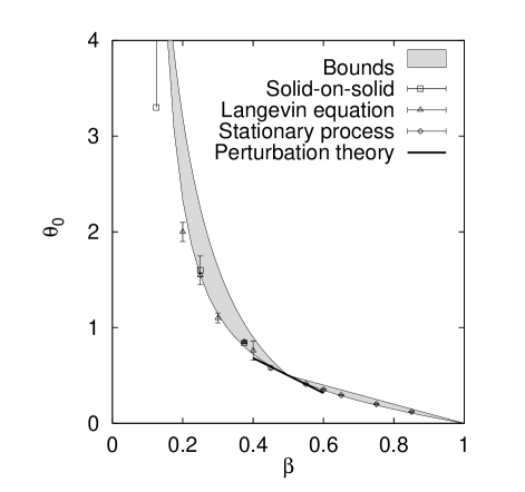
FIG. 5.: Summary of data for the transient exponent $\theta_{0}(\beta)$, obtained from simulations of the solid-on-solid models (squares), discretized Langevin equations (triangles) and the equivalent stationary process (diamonds). The bold line is the perturbation result (31), while the shaded area shows the range enclosed by the exact upper and lower bounds derived in Section VI.

VI Exact numerical bounds for $\theta_{0}$

In Section II several rigorous analytic bounds for $\theta_{0}$ were obtained by comparing the correlator $f_{0}(T)$ to a function with known persistence exponent and using Slepian’s theorem [3]. Having convinced ourselves, in the preceding section, that the expression (6) for $\theta_{S}$ is in fact exact in the whole interval $0<\beta<1$, we can now employ the same strategy to obtain further bounds by comparing $f_{0}(T,\beta)$ to $f_{S}(T,\beta)$. These bounds turn out to be very powerful because $f_{0}(T,\beta)$ and $f_{S}(T,\beta)$ share the same type of singularity at $T=0$ (see eqn.(14)).

Let $f_{A}(T)$ and $f_{B}(T)$ be monotonically decreasing functions with the same class of analytical behaviour near $T=0$. There will always exist numbers $b_{\rm min}$ and $b_{\rm max}$ such that $f_{A}(b_{\rm max}T)\leq f_{B}(T)\leq f_{A}(b_{\rm min}T)$ is satisfied for all $T$. Since the persistence exponent for a process with correlation function $f_{A}(bT)$ is just $b\theta_{A}$, where $\theta_{A}$ is the persistence exponent for the process with correlation function $f_{A}(T)$, we can deduce from Slepian’s theorem that $b_{\rm\min}\theta_{A}\leq\theta_{B}\leq b_{\rm\max}\theta_{A}$. We may therefore find upper and lower bounds for the persistence exponent of a given process if we know the persistence exponent for another process in the same class. In particular, we may use the result (6) for $\theta_{S}$ to obtain bounds for $\theta_{0}$.

Finding by analytic means the most restrictive values of $b_{\rm min}$ and $b_{\rm max}$ such that $f_{S}(b_{\rm max}T,\beta)\leq f_{0}(T,\beta)\leq f_{S}(b_{\rm min}T,\beta)$ is a formidable task. Our approach is to study the analytical behaviour near $T=0$ and $T=\infty$ to find values where the inequalities are satisfied in the vicinity of both limits, and then investigate numerically whether the inequalities are satisfied away from these asymptotic regimes. The same leading small-$T$ behaviour is obtained for $f_{S}(bT,\beta)$ and $f_{0}(T,\beta)$ when $b=2^{{1\over 2\beta}-1}$, and the same large-$T$ behaviour is found when $b=(1-\beta)/\beta$ for $\beta<1/2$ and $b=1$ for $\beta>1/2$. We conclude that

$$b_{\rm min} \leq \left\{\begin{array}[]{l c}\hbox{min}\left(2^{{1\over 2\beta}-1},{1\over\beta}-1\right)&\hbox{ for $\beta<1/2$}\\ 2^{{1\over 2\beta}-1}&\hbox{ for $\beta>1/2$}\end{array}\right.$$ (58)

$$b_{\rm max} \geq \left\{\begin{array}[]{l c}\hbox{max}\left(2^{{1\over 2\beta}-1},{1\over\beta}-1\right)&\hbox{ for $\beta<1/2$}\\ 1&\hbox{ for $\beta>1/2$}\end{array}\right.$$ (61)

Surprisingly, we find in the majority of cases that the inequalities (58) and (61) are satisfied as equalities. Specifically, in the cases where the corrections to the leading analytic behaviour has the appropriate sign to ensure that $f_{S}(bT,\beta)$ is a bound for $f_{0}(T,\beta)$ in both limits $T\to 0$ and $T\to\infty$, then numerical investigation revealed it to be a bound for all $T$. We are therefore able in the following cases to quote the most restrictive bounds and their region of applicability in analytical form, although the validity of the bounds has only been established numerically.

$$\theta_{0} \geq {(1-\beta)^{2}\over\beta}\qquad\hbox{ for $0<\beta<\beta_{1}(=0.1366\dots)$}$$ (62)

$$\theta_{0} \geq (1-\beta)2^{{1\over 2\beta}-1}\qquad\hbox{ for $\beta_{1}<\beta<{1\over 2}$}$$ (63)

$$\theta_{0} \leq {(1-\beta)^{2}\over\beta}\qquad\hbox{ for $\beta_{2}(=0.1549\dots)<\beta<{1\over 2}$}$$ (64)

$$\theta_{0} \leq 1-\beta\qquad\hbox{ for $\beta>{1\over 2}$}$$ (65)

The two critical values $\beta_{1}=0.1366\dots$ and $\beta_{2}=0.1549\dots$ correspond to the solutions in $]0,0.5[$ of ${1\over\beta_{1}}-1=2^{{1\over 2\beta_{1}}-1}$ and $\beta_{2}=2^{2\beta_{2}-3}$ respectively. Note that (65) coincides with the rigorous result in Eq. (21)

For other values of $\beta$, the sign of the leading corrections implies that (58) and (61) is only satisfied as an inequality, and the best value of the bound has to be obtained numerically by finding the value of $b$ where $f_{S}(bT,\beta)$ touches $f_{0}(T,\beta)$ at a point.

It is also possible to obtain bounds on $\theta_{0}(\beta)$ by comparing $f_{0}(T,\beta)$ with $f_{S}(bT,\beta^{\prime})$, where $\beta^{\prime}\neq\beta$. Consideration of the behaviour at small-$T$ shows that a lower bound on $\theta_{0}$ may be obtained when $\beta^{\prime}>\beta$, whereas an upper bound may be obtained for $\beta^{\prime}<\beta$. In the majority of cases, it can be shown that the most restrictive bounds are in fact obtained by $\beta^{\prime}=\beta$. For instance, consideration of the large-$T$ behaviour for $0<\beta<\beta_{1}$ shows that $b_{\rm min}\leq{1\over\beta^{\prime}}-1$, so $\theta_{\rm min}\leq\left({1\over\beta^{\prime}}-1\right)(1-\beta).$ Therefore, since this inequality is satisfied as an equality for $\beta^{\prime}=\beta$ (see (62)), and $\beta^{\prime}\geq\beta$, the best bound is obtained when $\beta^{\prime}=\beta$. Similarly, the inequalities (64) and (65) can be shown to be the best obtainable by this method. However, for $\beta_{1}<\beta<1/2$, a perturbative consideration with $\beta^{\prime}=\beta+\epsilon$ shows that a larger value of $\theta_{\rm min}$ may be obtained for $\epsilon$ small and positive, so (63) is not the best bound that may be obtained. A numerical investigation shows that the optimal value of $\beta^{\prime}$ is nevertheless very close to $\beta$, and an improvement in $\theta_{\rm min}$ of no more than $\approx 3\%$ was so obtained. For $\beta$ outside the ranges quoted in (62–65), it was found by numerical investigation that $\beta=\beta^{\prime}$ gave the best bound.

Numerical values of these bounds are listed in Table I, for comparison with the simulation data. The contents of the last three columns of this table are also plotted in Figure 5. The upper and lower bounds are (perhaps) surprisingly close together. Notice that the lower bound for $\theta_{0}$ when $\beta=0.125$ is $6.125$, whereas the discrete solid-on-solid simulations yielded the inconclusive value $>3.3$. All the other data are consistent with the bounds, within numerical error. It is interesting to note that the data, as well as the exact perturbation theory result, tend to lie much closer to the lower than the upper bound.

VII Conclusions

In this paper we have investigated the first passage statistics for a one-parameter family of non-Markovian, Gaussian stochastic processes which arise in the context of interface motion. We have identified two persistence exponents describing the short time (transient) and long time (steady state) regimes, respectively.

For the steady state exponent the previously conjectured relation $\theta_{S}=1-\beta$ [7] was confirmed. While this relation follows from simple scaling arguments applied to the original process, it is rather surprising when viewed from the perspective of the equivalent stationary process with autocorrelation function (13): It provides the exact decay exponent for a family of correlators whose class $\alpha=2\beta$ (in the sense of Slepian [3]) covers the whole interval $\alpha\in]0,2[$; previous exact results were restricted to $\alpha=1$ and $\alpha=2$ [3]. We have demonstrated in Section VI how this can be exploited to obtain accurate upper and lower bounds for other processes within the same class.

Estimates for the nontrivial transient exponent $\theta_{0}$ were obtained using a variety of analytic, exact and perturbative approaches, as well as from simulations. The numerical techniques – direct simulation of interface models and construction of realizations of the equivalent stochastic process, respectively – are complementary, in the sense that the former is restricted to the regime $\beta<1/2$, while the latter gives the most accurate results for $\beta>1/2$. The results summarized in Figure 5 provide a rather complete picture of the function $\theta_{0}(\beta)$.

Finally, we briefly comment on a possible experimental realization of our work. Langevin equations of the type (1) are now widely used to describe time-dependent step fluctuations on crystal surfaces observed with the scanning tunneling microscope [28]. From such measurements the autocorrelation function of the step position can be extracted, and different values of $\beta$ have been observed, reflecting different dominant mass transport mechanisms [29]. Thus it seems that, perhaps with a slight refinement of the observation techniques, the first passage statistics of a fluctuating step may also be accessible to experiments.

Acknowledgements

The authors gratefully acknowledge the hospitality of ICTP, Trieste, during a workshop at which this research was initiated. J.K. wishes to thank Alex Hansen for comments, and the DFG for support within SFB 237 Unordnung und grosse Fluktuationen. Laboratoire de Physique Quantique is Unité Mixte de Recherche C5626 of Centre National de la Recherche Scientifique (CNRS).

Appendix: Derivation of some exponent inequalities

To establish (20) we need to show that $f_{S}(T)\geq\exp(-|T|/2)$ for all $T$, provided that $\beta>1/2$. To this end we rewrite (13) in the form

$$f_{S}(T)=\frac{1}{2}e^{\beta|T|}[1+e^{-2\beta|T|}-(1-e^{-|T|})^{2\beta}]$$ (A1)

and notice that for $\beta>1/2$, $[1-\exp(-|T|)]^{2\beta}\leq 1-\exp(-|T|)$. Thus

$$f_{S}(T)\geq\frac{1}{2}[e^{-\beta|T|}+e^{-(1-\beta)|T|}]\geq e^{-|T|/2},$$ (A2)

where the last inequality follows from the fact that the expression in the square brackets is an increasing function of $\beta$ for $\beta>1/2$.

Next we consider the relations (21). We express (7) in the form

$$f_{0}(T)=2^{-2\beta}e^{\beta|T|}g(e^{-|T|})$$ (A3)

where the function $g$ is given by

$$g(y)=(1+y)^{2\beta}-(1-y)^{2\beta}.$$ (A4)

Taking two derivatives with respect to $y$ it is seen that $g^{\prime\prime}\geq 0$ for $\beta<1/2$ and $g^{\prime\prime}\leq 0$ for $\beta>1/2$. Since $g(0)=0$ and $g(1)=2^{2\beta}$ always, it follows that $g(y)$ is bounded by the linear function $2^{2\beta}y$, from above for $\beta<1/2$ and from below for $\beta>1/2$. Inserted back into (A3) this implies

$$f_{0}(T)\leq e^{-(1-\beta)|T|}\;\;{\rm for}\;\;\beta<1/2$$

$$f_{0}(T)\geq e^{-(1-\beta)|T|}\;\;{\rm for}\;\;\beta>1/2,$$ (A5)

and (21) follows by applying Slepian’s theorem [3] in conjunction with the fact that $\theta=\lambda$ for purely exponential (Markovian) correlators.

The inequalities (22) are a little more subtle to prove. Let us first consider the case ${1/2}<\beta<1$. We need to prove that $f_{0}(T)\geq f_{S}(T)$ for all $T$. Then the relation ${\theta}_{0}\leq{\theta}_{S}$ will follow from Slepian’s theorem. Denoting $y=e^{-|T|}$ and using the expressions of $f_{0}(T)$ and $f_{S}(T)$, we then need to prove that the function $F(y)=(1+y)^{2\beta}+(a-1)(1-y)^{2\beta}-a(y^{2\beta}+1)$ (where $a=2^{2\beta-1}$) is positive for all $0\leq y\leq 1$.

First we note, by simple Taylor expansion around $y=0$ and $y=1$, that $F(y)>0$ for $y$ close to $0$ and $1$. The first derivative, $F^{\prime}(y)$ starts at the positive value $2\beta(2-a)$ at $y=0$ and approaches $0$ from the negative side as $y\to 1^{-}$. The second derivative $F^{\prime\prime}(y)$ starts at $-\infty$ as $y\to 0^{+}$ and approaches $+\infty$ as $y\to 1^{-}$. We first show that $F^{\prime\prime}(y)$ is a monotonically increasing function of $y$ in $0\leq y\leq 1$.

To establish this, we consider the third derivative, $F^{\prime\prime\prime}(y)=2\beta(2\beta-1)(2\beta-2)G(y)$, where

$$G(y)=(1+y)^{2\beta-3}-(a-1)(1-y)^{2\beta-3}-ay^{2\beta-3}.$$ (A6)

Now, since $(1+y)^{(2\beta-3)}<y^{(2\beta-3)}$ for all $0\leq y\leq 1$, we have $G(y)<-(a-1)[y^{2\beta-3}+(1-y)^{2\beta-3}]$ implying $G(y)<0$ for $0\leq y\leq 1$. Since $1/2\leq\beta\leq 1$, it follows that $F^{\prime\prime\prime}(y)>0$ for all $0\leq y\leq 1$. Therefore, $F^{\prime\prime}(y)$ is a monotonically increasing function of $y$ for $0\leq y\leq 1$ and hence crosses zero only once in the interval $[0,1]$. This implies that the first derivative $F^{\prime}(y)$ has one single extremum in $[0,1]$. However, since $F^{\prime}(y)$ starts from a positive value at $y=0$ and approaches $0$ from the negative side as $y\to 1^{-}$, this single extremum must be a minimum. Therefore, $F^{\prime}(y)$ crosses zero only once in $[0,1]$ implying that the function $F(y)$ has only a single extremum in $[0,1]$. Since, $F(y)$ for $y\to 0^{+}$ and $y\to 1^{-}$, this must be a maximum. Furthermore, $F(y)$ can not cross zero in $[0,1]$ because that would imply more than one extremum which is ruled out. This therefore proves that $f_{0}(T)\geq f_{S}(T)$ for all $T$ for $\beta\geq 1/2$ and hence, using Slepian’s theorem, $\theta_{0}\leq\theta_{S}$. Using similar arguments, it is easy to see that the reverse, $\theta_{0}\geq\theta_{S}$ is true for $\beta\leq 1/2$.

Finally we prove the inequality (17) which relates the values of $\theta_{0}$ for two different exponents $\beta$ and $\beta^{\prime}>\beta$, subject to an additional constraint to be specified below. In the same spirit as above, one can show that after defining $\gamma=(1-\beta)/(1-\beta^{\prime})>1$, one obtains

$$f_{0}(T,\beta) \leq f_{0}(\gamma T,\beta^{\prime})$$ (A8)

$$\hbox{ for }\beta<\beta^{\prime}\hbox{ and }\beta 2^{-2\beta}\leq\beta^{\prime}2^{-2\beta^{\prime}}.$$

Both functions in (A8) decay exponentially at large time with the same decay rate $\lambda_{0}=1-\beta=\gamma(1-\beta^{\prime})$, such that their ratio approaches a constant when $T\to\infty$. The last condition $\beta 2^{-2\beta}\leq\beta^{\prime}2^{-2\beta^{\prime}}$ expresses that the limit of this ratio must be less than unity. As $f_{0}(T,\beta)\leq f_{0}(\gamma T,\beta^{\prime})$ in the vicinity of $T=0$ (this is just a consequence of $\beta<\beta^{\prime}$), and as a careful study shows that $\frac{d}{dT}[f_{0}(T,\beta)/f_{0}(\gamma T,\beta^{\prime})]$ has at most one zero in the range $]0,\infty[$, we conclude that $f_{0}(T,\beta)/f_{0}(\gamma T,\beta^{\prime})<1$ if and only if the limit of this ratio for $T\to\infty$ is less than unity. In practice, the last condition in (A8) expressing this constraint can be violated only if $\beta>1/2$ and $\beta^{\prime}>(2\ln 2)^{-1}\approx 0.7213475...$.

Using Slepian’s theorem, and the fact that the persistence exponent associated with $f_{0}(\gamma T,\beta)$ is exactly $\gamma$ times the persistence exponent associated with $f_{0}(T,\beta)$ [3], we arrive at the inequality (17) which holds under the conditions stated in (A8). Setting $\beta$ or $\beta^{\prime}$ equal to $1/2$ (keeping $\beta<\beta^{\prime}$), eq.(17) reduces to the bounds (21).

For $\beta^{\prime}>\beta>1/2$ the inequality (17) comes rather close to being satisfied as an equality. For example, setting $\beta=0.55$, $\beta^{\prime}=0.85$ eq.(17) requires that $\theta_{0}(\beta)/\theta_{0}(\beta^{\prime})\geq 3$, while the numerical data in Table I yield $\theta_{0}(\beta)/\theta_{0}(\beta^{\prime})=3.39$. The only pair of values in Table I which violates the inequality (17) is $(\beta,\beta^{\prime})=(0.75,0.85)$. Since for these values the condition $\beta 2^{-2\beta}\leq\beta^{\prime}2^{-2\beta^{\prime}}$ is also violated, this may be taken as an indication that the numerical estimates for $\beta>1/2$ are rather accurate.

$\beta$		$\theta_{S}$	$1-\beta$		$\theta_{0}$	$\theta_{\rm min}$	$\theta_{\rm max}$
0.125(∗)	$0.86$	$\pm 0.02$	0.875	$>3.3$		6.125	7.359
0.2	$0.788$	$\pm 0.01$	0.8	$2.0$	$\pm 0.1$	2.333	3.200
0.25(∗)	$0.754$	$\pm 0.01$	0.75	$1.6$	$\pm 0.15$	1.547	2.250
0.25	$0.740$	$\pm 0.01$	0.75	$1.55$	$\pm 0.02$	1.547	2.250
0.3	$0.69$	$\pm 0.01$	0.7	$1.10$	$\pm 0.05$	1.141	1.633
0.375(∗)	$0.635$	$\pm 0.01$	0.625	$0.84$	$\pm 0.01$	0.801	1.042
0.375	$0.625$	$\pm 0.01$	0.625	$0.85$	$\pm 0.01$	0.801	1.042
0.4	$0.60$	$\pm 0.01$	0.6	$0.76$	$\pm 0.1$	0.723	0.900
0.45	$0.53$	$\pm 0.01$	0.55	$0.58$	$\pm 0.02$	0.598	0.672
0.55	$0.44$	$\pm 0.01$	0.45	$0.41$	$\pm 0.01$	0.415	0.450
0.6	$0.39$	$\pm 0.01$	0.4	$0.35$	$\pm 0.01$	0.348	0.400
0.65	$0.346$	$\pm 0.005$	0.35	$0.295$	$\pm 0.005$	0.289	0.350
0.75	$0.247$	$\pm 0.005$	0.25	$0.201$	$\pm 0.005$	0.191	0.250
0.85	$0.150$	$\pm 0.005$	0.15	$0.121$	$\pm 0.005$	0.107	0.150

Table I. Numerical estimates of the persistence exponents $\theta_{S}$ and $\theta_{0}$, compared to the fractional Brownian motion result $\theta_{S}=1-\beta$ (third column) and to the optimal bounds $\theta_{\rm min}$ and $\theta_{\rm max}$ derived in Section VI (last two columns). With the exception of the values marked with an asterisk^(∗), which were obtained using discrete solid-on-solid models (Section IV.A), the data for $\beta\leq 0.40$ are taken from simulations of discretized Langevin equations (Section IV.B) while those for $\beta\geq 0.45$ were generated using the equivalent stationary Gaussian process (Section IV.C). In all cases the error bars reflect a subjective estimate of systematic errors.

REFERENCES

- [1] B. Derrida, A.J. Bray and C. Godrèche, J. Phys. A 27, L357 (1994); B. Derrida, V. Hakim and V. Pasquier, Phys. Rev. Lett. 75, 751 (1995), and J. Stat. Phys. 85, 763 (1996).
- [2] S.N. Majumdar, C. Sire, A.J. Bray and S.J. Cornell, Phys. Rev. Lett. 77, 2867 (1996) [cond-mat/9605084]; B. Derrida, V. Hakim and R. Zeitak, ibid. 2871 [cond-mat/9606005].
- [3] D. Slepian, Bell Syst. Tech. J. 41, 463 (1962).
- [4] M. Kac, SIAM Review 4, 1 (1962); I.F. Blake and W.C. Lindsey, IEEE Trans. Information Theory 19, 295 (1973).
- [5] S.N. Majumdar and C. Sire, Phys. Rev. Lett. 77, 1420 (1996) [cond-mat/9604151].
- [6] For a review of linear Langevin equations for interfaces see J. Krug, in Scale Invariance, Interfaces, and Non-Equilibrium Dynamics, ed. by A. McKane et al. (Plenum Press, New York 1995), pp.25.
- [7] J. Krug and H.T. Dobbs, Phys. Rev. Lett. 76, 4096 (1996).
- [8] B.B. Mandelbrot and J.W. van Ness, SIAM Review 10, 422 (1968).
- [9] T.J. Newman and A.J. Bray, J. Phys. A 23, 4491 (1990).
- [10] S.O. Rice, Bell Systems Technical Journal vols. 23 and 24, reproduced in Noise and Stochastic Processes, edited by N. Wax (Dover 1954).
- [11] K. Oerding, S.J. Cornell, and A.J. Bray, to appear in Phys. Rev. E (1997) [cont-mat/9702203].
- [12] For a realistic estimate of the required relaxation time it is useful to know also the prefactor of the relation . This is available analytically for the Arrhenius model () [13] and numerically for the curvature model () [6]. In the steady state simulations reported here we chose for the –models (system size ), and for the –model (system size ).
- [13] J. Krug, H.T. Dobbs and S. Majaniemi, Z. Phys. B 97, 281 (1995).
- [14] Z. Rácz, M. Siegert, D. Liu and M. Plischke, Phys. Rev. A 43, 5275 (1991).
- [15] F. Family, J. Phys. A 19, L441 (1986).
- [16] J. Krug, Phys. Rev. Lett. 72, 2907 (1994); J.M. Kim and S. Das Sarma, ibid. 2903 (1994).
- [17] W. H. Press et. al., Numerical Recipes, Cambridge University Press.
- [18] N.-N. Pang, Y.-K. Yu and T. Halpin-Healy, Phys. Rev. E 52, 3224 (1995).
- [19] S.M. Berman, Ann. Math. Stat. 41, 1260 (1970).
- [20] A. Hansen, T. Engøy and K.J. Måløy, Fractals 2, 527 (1994).
- [21] M. Ding and W. Yang, Phys. Rev. E 52, 207 (1995).
- [22] S. Maslov, M. Paczuski and P. Bak, Phys. Rev. Lett. 73, 2162 (1994).
- [23] K.J. Falconer, The Geometry of Fractal Sets (Cambridge University Press, 1985).
- [24] S. Orey, Z. Wahrscheinlichkeitstheorie verw. Geb. 15, 249 (1970).
- [25] M.B. Marcus, Z. Wahrscheinlichkeitstheorie verw. Geb. 34, 279 (1976).
- [26] A. Barbé, IEEE Trans. Information Theory 38, 814 (1992).
- [27] S.C. Lim and V.M. Sithi, Phys. Lett. A 206, 311 (1995).
- [28] N.C. Bartelt, T.L. Einstein and E.D. Williams, Surf. Sci. 312, 411 (1994).
- [29] N.C. Bartelt, J.L. Goldberg, T.L. Einstein, E.D. Williams, J.C. Heyraud and J.J. Métois, Phys. Rev. B 48, 15453 (1993); L. Kuipers, M.S. Hoogeman and J.W.M. Frenken, Phys. Rev. Lett. 71, 3517 (1993); M.. Giesen-Seibert, R. Jentjens, M. Poensgen and H. Ibach, ibid. 3521.