Finite temperature spectral-functions of strongly correlated
one-dimensional electron systems

Abstract

The spectral functions of $tJ$ and $tJ_{XY}$ models in the limit of $J/t\rightarrow 0$ and at finite temperatures $T\ll t$ are calculated using the spin-charge factorized wave function. We find that the Luttinger-liquid like scaling behavior for a finite system with $L$ sites is restricted below temperatures of the order $T\lesssim J/L$. We also observe weight redistribution in the photoemission spectral function in the energy range $t$, which is much larger than the temperature.

Single-particle spectral functions are very useful to understand the electronic structure of solids. They are measured in photoemission [$B(k,\omega)$] and inverse photoemission [$A(k,\omega)$] experiments. For actual calculations, the Lehmann representation is very useful:

$$B(k,\omega)=\frac{1}{Z}\sum_{i,f,\sigma}\left|\langle f|a^{\phantom{\dagger}}_{k,\sigma}|i\rangle\right|^{2}\delta(\omega-E_{i}+E_{f})e^{-\beta E_{i}},$$ (1)

where $i$ and $f$ denote the initial and final states with $N$ and $N-1$ electrons, respectively, and $a_{k,\sigma}$ annihilates an electron with momentum $k$ and spin $\sigma$. Furthermore, $Z=\sum_{i}e^{-\beta E_{i}}$ is the partition function with $\beta=1/T$ being the inverse temperature. A similar expression holds for $A(k,\omega)$, which we will not treat in this paper.

In contrast to quasiparticles in usual three-dimensional Fermi liquids, the collective excitations of one-dimensional interacting electrons[3] give rise to anomalous scaling behavior of the one-particle Green’s function[4] with non-universal exponents. For example, the momentum distribution function $n_{k}=\frac{1}{2}\int d\omega B_{\sigma}(k,\omega)$ takes the form $n_{k}\approx n_{F}+{\rm sgn}(k-k_{F})|k-k_{F}|^{\alpha}$ near the Fermi momentum $k_{F}$ and zero temperature, where the exponent $\alpha$ depends on the actual model and coupling constants. Similarly, the local spectral function (single-particle density of states) $B(\omega)=\frac{1}{L}\sum_{k}B(k,\omega)$ also scales with a power law:[5] $B(\omega)\propto|\omega-\varepsilon_{F}|^{\alpha}$. To describe this critical behavior of one-dimensional models at low energies, Haldane introduced the fruitful concept of Luttinger liquids.[6] Following a different approach, conformal field theory tells us that the exponents are related to the finite size corrections of the energy.[7, 8]

Recent experiments on quasi one dimensional materials raised the question if this behavior can be observed.[9, 10] Furthermore, in these experiments an anomalous spectral weight transfer has been observed: changing the temperature by 100 K, one can observe weight redistribution on the scale of 1 eV, which is a hundred times larger than the temperature. In this paper we will try to explain this behavior in a simple way.

We are considering the isotropic and anisotropic $tJ$ model, defined by the Hamiltonian

$$H_{tJ} = -t\sum_{i,\sigma}(\tilde{a}_{i,\sigma}^{\dagger}\tilde{a}_{i+1,\sigma}^{\vphantom{\dagger}}+{\rm H.c.})$$ (3)

$$+\sum_{i}\sum_{\alpha=x,y,z}J^{\alpha}\left(S_{i}^{\alpha}S_{i+1}^{\alpha}-\frac{1}{4}\delta_{\alpha,z}n_{i}n_{i+1}\right),$$

in the limit of small exchange $J^{\alpha}\rightarrow 0$, where $\tilde{a}_{i,\sigma}$ are the usual projected operators to exclude double occupancy. Actually, the Hubbard model in the large-$U$ limit can be mapped onto a strong coupling model usually identified as the $tJ$ model plus three-site terms using a canonical transformation,[11] where $J=4t^{2}/U$ is small. The spectral function of the Hubbard model has been studied using exact diagonalization[12] and Quantum Monte Carlo [13] techniques, which both have well known limitations.

An alternative, powerful but model limited approach is based on the special property of the wave functions of the Hubbard model in the limit of large Coulomb repulsion[14] (also for $J/t\rightarrow 0$ in the $tJ$ model), that the wave function factorizes:

$$|i\rangle=|\psi^{\prime}\rangle\otimes|\chi^{\prime}\rangle.$$ (4)

This has allowed the calculation and confirmation of the power law behavior of the static correlation function $n_{k}$ and gave[15] $\alpha=1/8$. $|\psi^{\prime}\rangle$ describes the charge degrees of freedom and is a wave function of free spinless fermions with momenta $k^{\prime}_{j}$, quantized as $Lk^{\prime}_{j}=2\pi{\cal I}^{\prime}_{j}+Q^{\prime}$, where ${\cal I}^{\prime}_{j}$ are distinct integers, $0\leq{\cal I}^{\prime}_{j}\leq L-1$ and $j=1,2,\dots,N$. Twisted boundary conditions are imposed by the momentum $Q^{\prime}$ of the spin wave function $|\chi^{\prime}\rangle$, which describes the spins on a squeezed lattice of $N$ sites and are eigenfunctions of a spin Hamiltonian with an effective spin exchange $\tilde{J}$ which depends on the actual charge wave function $|\psi^{\prime}\rangle$, and e.g. for the ground state $\tilde{J}^{\alpha}=J^{\alpha}n[1-\sin^{2}(\pi n)/(\pi n)^{2}]$, where $n=N/L$. We will take periodic boundary conditions to avoid edge effects[16] and an even number of electrons not a multiple of four (i.e. $N=2,6,10,\dots$) for convenience.

To calculate the thermal average, we need to know all the energies and wave functions of the spin model. Since for the Heisenberg model this is very difficult to obtain, we turn to the $XY$ model (i.e. $J^{z}=0$). In this special case, the spin model can be mapped onto noninteracting spinless fermions using the Wigner-Jordan transformation. Assuming that the occupied sites represent the $\uparrow$ spins, the states are characterized by $N_{\uparrow}$ integer numbers $0\geq{\cal J}^{\prime}_{j}\geq N-1$, and the momenta $q^{\prime}_{j}$ of the free spinless fermions representing the spins are quantized as $Lq^{\prime}_{j}=2\pi{\cal J}^{\prime}_{j}$. Finally, the momentum of the spin wave function determining the boundary condition of the charge part is $Q^{\prime}=\sum_{j=1}^{N_{\uparrow}}q^{\prime}_{j}=2\pi{\cal J}^{\prime}/N$, with ${\cal J}^{\prime}$ integer. The energy of the state is simply $E_{i}=E_{i,c}+E_{i,s}$, where $E_{i,c}=-2t\sum_{j=1}^{N}\cos k^{\prime}_{j}$ and $E_{i,s}=\tilde{J}_{XY}\sum_{j=1}^{N_{\uparrow}}\cos q^{\prime}_{j}$, while the momentum reads $P_{i}=\sum_{j=1}^{N}k^{\prime}_{j}$. One should note that despite the fact that both the charge and spin wave functions in Eq. (4) are those of free spinless fermions, the resulting wave function describes a nontrivial and strongly correlated system. As far as the exponent $\alpha$ (at $T=0$) is concerned, it changes from $\alpha=1/8$ in the isotropic case to $\alpha=1/4$ in the $XY$ case.[17]

Similarly, the final, $N-1$ electron wave function factorizes as well: $|f\rangle=|\psi\rangle\otimes|\chi\rangle$. The quantum numbers for the spinless fermions representing the charges are ${\cal I}_{j}$, and the corresponding momenta $Lk_{j}=2\pi{\cal I}_{j}+Q$. Here $Q=2\pi{\cal J}/(N-1)$ is the momentum of the $N-1$ spin wave function, ($0\geq{\cal J}\geq N-2$).

Since the charge and the spin part are coupled through the momentum $Q^{\prime}$ of the spin wave function, the partition function does not factorize[18] (i.e. the free energy is not a sum of charge and spin contribution) and it will read $Z=\sum_{Q^{\prime}}Z_{c}(Q^{\prime})Z_{s}(Q^{\prime})$, where

$\displaystyle Z_{c}(Q^{\prime})=\sum_{\{{\cal I}^{\prime}_{j}\}}e^{-\beta E_{i,c}},\quad Z_{s}(Q^{\prime})=\sum_{\{{\cal J}^{\prime}_{j}\}_{Q^{\prime}}}e^{-\beta E_{i,s}},$

and the sum in $Z_{s}$ is over the states with given momentum $Q^{\prime}$. In calculating the thermodynamic averages, one can work in principle in an ensemble fixing either the magnetization or the magnetic field. We have used both ensembles, and although the results in the thermodynamic limit should be independent of the ensemble we choose, there are strong finite size effects.

Even though we know all the excitations for the $tJ_{XY}$ model, we will make further restrictions which are needed to perform calculations on reasonably large system sizes: Namely, we will consider temperatures much smaller than the energy scale of the charges. In other words, for the charge part we neglect the excitations and take the ground state given by consecutive integers $\{{\cal I}^{\prime}\}=\{-N/2,-N/2+1,\dots,N/2-1\}$. Then the remaining free parameter is $T/\tilde{J}$, and all the temperature dependence is now in the spin part. Furthermore, since the energy of the charge part also depends on $Q^{\prime}$ as $E_{i,c}(Q^{\prime})-E_{i,c}(Q^{\prime}=\pi)=\frac{1}{2\pi L}u_{c}(Q^{\prime}-\pi)^{2}$, where $u_{c}\propto t$ is the charge velocity, we will assume that the momentum of the spin part in the initial $N$ electron state is $Q^{\prime}=\pi$. This restriction is actually more for convenience, as the result does not depend on this assumption - we will comment on this later on.

Using the factorized wave function, the spectral function defined in Eq. (1) simplifies to[19]

$$B(k,\omega)=\sum_{Q,\sigma}D_{\sigma}(Q,\beta)B_{Q}(k,\omega).$$ (5)

Here $B_{Q}(k,\omega)=B_{Q,Q^{\prime}=\pi}(k,\omega)$ depends on the spinless fermion wave function only:

$$B_{Q,Q^{\prime}}(k,\omega) = L\sum_{\{I\}}\left|\langle\psi_{Q}|b^{\phantom{\dagger}}_{0}|\psi^{\prime}_{Q^{\prime}}\rangle\right|^{2}$$ (7)

$$\times\delta(\omega-E_{i,c}+E_{f,c})\delta_{k,P_{i}\!-\!P_{f}},$$

where $b_{0}$ annihilates a spinless fermion at site $0$. The matrix elements in $B_{Q,Q^{\prime}}(k,\omega)$ read:

$$L\left|\langle\psi_{Q}|b^{\phantom{\dagger}}_{0}|\psi^{\prime}_{Q^{\prime}}\rangle\right|^{2}=L^{-2N+2}\sin^{2N-2}\frac{Q^{\prime}\!-\!Q}{2}$$ (8)

$$\times\prod_{j>i}\sin^{2}\frac{k_{j}\!-\!k_{i}}{2}\prod_{j>i}\sin^{2}\frac{k^{\prime}_{j}\!-\!k^{\prime}_{i}}{2}\prod_{i,j}\sin^{-2}\frac{k^{\prime}_{i}\!-\!k_{j}}{2}.$$ (9)

We can actually recognize Anderson’s orthogonality catastrophe[20] in these complicated matrix elements, which is a consequence of changing the boundary condition from $Q$ to $Q^{\prime}$ in the charge wave function due to momentum transferred to the spins.

On the other hand, the contribution of the spin degrees of freedom[21, 19] $D_{\sigma}(Q,\beta)=D_{\sigma}(Q,Q^{\prime}=\pi,\beta)$ is given by

$\displaystyle D_{\sigma}(Q,Q^{\prime},\beta)=\frac{1}{N-1}\frac{1}{Z_{s}}\sum_{m,\{{\cal J^{\prime}}\}_{Q^{\prime}}}\omega_{0\rightarrow m,\sigma}e^{im(Q^{\prime}-Q)}e^{-\beta E_{i,s}},$

where $\omega_{0\rightarrow m,\sigma}$ denotes the amplitude to transfer a $\sigma$ spin from site $0$ to $m$:

$$\omega_{0\rightarrow m,\sigma}=\langle\chi^{\prime}|\hat{P}_{m,m-1}\dots\hat{P}_{1,0}n_{0}|\chi^{\prime}\rangle.$$ (10)

The operator $\hat{P}_{j,j+1}=2{\bf S}_{j}{\bf S}_{j+1}+\frac{1}{2}$ permutes the spins on sites $j$ and $j+1$.

a Spin part:

For the $XY$ model, after introducing the spinless fermions (with operators $f$) in the Wigner-Jordan transformation, the permutation operator reads

$\displaystyle\hat{P}_{j+1,j}=n_{j+1}n_{j}+f^{\dagger}_{j+1}f^{\phantom{\dagger}}_{j}+(1\!-\!n_{j+1})(1\!-\!n_{j})+f^{\dagger}_{j}f^{\phantom{\dagger}}_{j+1},$

and the spin transfer amplitude can be easily calculated from Eq. (10) using Wick’s theorem. We find that

$\displaystyle\omega_{0\rightarrow m,\uparrow}=\left|\begin{array}[]{cccc}g_{0}&g_{1}&\dots&g_{m}\\ 1\!+\!g_{-1}&g_{0}&\dots&g_{m-1}\\ 1\!+\!g_{-2}&1\!+\!g_{-1}&\dots&g_{m-2}\\ \vdots&\vdots&&\vdots\\ 1\!+\!g_{-m}&1\!+\!g_{1-m}&\dots&g_{0}\\ \end{array}\right|,$

where $g_{l}=(-1)^{l}\langle\chi|f^{\dagger}_{l}f^{\phantom{\dagger}}_{0}|\chi\rangle=\frac{1}{N}\sum_{j=1}^{N_{\uparrow}}e^{i(\pi-q^{\prime}_{j})l}$. In particular, $g_{0}=N_{\uparrow}/N$ and $g_{-j}=g_{j}^{*}$, furthermore the relation $\omega_{0\rightarrow N-1-m,\sigma}=e^{iQ^{\prime}}\omega^{*}_{0\rightarrow m,\sigma}$ holds.

For large temperatures $t\gg T\gg\tilde{J}$ (equivalent to “hot spins” of Ref. [22]) a high temperature expansion is possible: if we relax the constraint that we take only states with momenta $Q^{\prime}$, then it follows that $Z_{s}=2^{N}+O(\beta J_{XY})$ and for $\omega_{0\rightarrow m,\sigma}$ we have to count the number of states where the first $m+1$ spins have $S^{z}=\uparrow$, which is $2^{N-m-1}$. Working in a subspace with definite momentum $Q^{\prime}$, each subspace will acquire roughly $1/N$ of the values given above (the actual distribution depends on how many states are in a given $Q^{\prime}$ subspace), and in the thermodynamic limit we get

$$D_{\sigma}(Q,Q^{\prime},\beta\rightarrow 0)=\frac{1}{N-1}\frac{3}{10-8\cos(Q-Q^{\prime})}.$$ (11)

This result is not only valid for the $XY$ model, but also for the isotropic Heisenberg model.

We show the behavior of the spin part in Fig. 1. Apart from the clear power-law singularity near $Q=\pi/2$ at zero temperature, we observe that at fixed small temperature this behavior disappears as we increase the system size. This indicates that the singularity will vanish for any finite temperature in the thermodynamic limit. Also there is a difference between calculating $D_{\sigma}(Q,\beta)$ in the two ensembles mentioned above, however the finite size effects are decreasing with increasing $N$. Let us also note that the sum rule $\sum_{Q}D_{\sigma}(Q,\beta)=N_{\sigma}/N$ is satisfied for any temperature. Furthermore, $D_{\sigma}(Q,Q^{\prime},\beta)\approx D_{\sigma}(Q-Q^{\prime}+\pi,\beta)$ in the thermodynamic limit.

FIG. 1.: Temperature dependence of $D_{\sigma}(Q,\beta)$ for the $XY$ model in zero magnetic field (solid) and zero magnetization (empty symbols) for $T/\tilde{J}=0$, 0.5 and $T\gg\tilde{J}$. The solid line for $T=0$ shows the $N=250$ result, and for $T\gg\tilde{J}$ Eq. (11) is plotted.

b Momentum distribution function:

From Eq. (5) we get:

$$n_{k}=\sum_{Q}B_{Q}(k)D_{\sigma}(Q,\beta).$$ (12)

To calculate $n_{k}$ efficiently, we have to find a convenient way to evaluate $B_{Q}(k)$. For that reason, let us follow Ref. [15]: In the alternative representation of the momentum distribution

$\displaystyle n_{k}=\frac{1}{Z}\sum_{i}\sum_{l=0}^{L-1}\langle i|a^{\dagger}_{l,\sigma}a^{\phantom{\dagger}}_{0,\sigma}|i\rangle e^{ikl}e^{-\beta E_{i}}$

we replace $|i\rangle$ by the factorized wave function, Eq. (4):

$$\langle i|a^{\dagger}_{l,\sigma}a^{\phantom{\dagger}}_{0,\sigma}|i\rangle=\sum_{m=0}^{N-2}\langle\psi^{\prime}|c^{\dagger}_{l}\delta_{N_{l}-m}c^{\phantom{\dagger}}_{0}|\psi^{\prime}\rangle\omega_{0\rightarrow m,\sigma},$$ (13)

where $N_{l}=\sum_{l^{\prime}=0}^{l}n_{l^{\prime}}$ counts the number of spinless fermions between sites $0$ and $l$, and $\omega_{0\rightarrow m,\sigma}$ is calculated for the particular $|\chi^{\prime}\rangle$. Now, replacing $\delta_{N_{l}-m}$ by its Fourier representation:

$\displaystyle\delta_{N_{l}-m}=\frac{1}{N-1}\sum_{Q}e^{i(Q-Q^{\prime})(N_{l}-m)},$

and comparing Eqs. (12) and (13), we get

$$B_{Q,Q^{\prime}}(k)=\sum_{l}e^{ikl}\langle\psi^{\prime}|c^{\dagger}_{l}\prod_{l^{\prime}=1}^{l-1}e^{in_{l^{\prime}}(Q-Q^{\prime})}c^{\phantom{\dagger}}_{0}|\psi^{\prime}\rangle.$$ (14)

This can be further simplified using the identity $e^{in_{l}(Q-Q^{\prime})}=1+xn_{l}$, where we introduced $x=e^{i(Q-Q^{\prime})}-1$, so that $\langle\psi^{\prime}|c^{\dagger}_{l}\prod_{l^{\prime}=1}^{l-1}e^{in_{l^{\prime}}(Q-Q^{\prime})}c^{\phantom{\dagger}}_{0}|\psi^{\prime}\rangle$ in Eq. (14) is equal to

$\displaystyle\left|\begin{array}[]{cccc}\langle c^{\dagger}_{l}c^{\phantom{\dagger}}_{0}\rangle&\langle c^{\dagger}_{l}c^{\phantom{\dagger}}_{1}\rangle&\dots&\langle c^{\dagger}_{l}c^{\phantom{\dagger}}_{l-1}\rangle\\ x\langle c^{\dagger}_{1}c^{\phantom{\dagger}}_{0}\rangle&1\!+\!x\langle c^{\dagger}_{1}c^{\phantom{\dagger}}_{1}\rangle&\dots&x\langle c^{\dagger}_{1}c^{\phantom{\dagger}}_{l-1}\rangle\\ x\langle c^{\dagger}_{2}c^{\phantom{\dagger}}_{0}\rangle&x\langle c^{\dagger}_{2}c^{\phantom{\dagger}}_{1}\rangle&\dots&x\langle c^{\dagger}_{1}c^{\phantom{\dagger}}_{l-1}\rangle\\ \vdots&\vdots&&\vdots\\ \\ x\langle c^{\dagger}_{l-1}c^{\phantom{\dagger}}_{0}\rangle&x\langle c^{\dagger}_{l-1}c^{\phantom{\dagger}}_{1}\rangle&\dots&1\!+\!x\langle c^{\dagger}_{l-1}c^{\phantom{\dagger}}_{l-1}\rangle\end{array}\right|,$

where $\langle c^{\dagger}_{l}c^{\phantom{\dagger}}_{l^{\prime}}\rangle=\frac{1}{L}\sum_{j}e^{-ik^{\prime}_{j}(l-l^{\prime})}$. Using this equation, we are able to compute $B_{Q}(k,\omega)$ for systems with a few hundred sites. It turns out that $B_{Q,Q^{\prime}}(k,\omega)=B_{Q-Q^{\prime}+\pi}(k,\omega)$ apart from some small finite size corrections, therefore our assumption to fix $Q^{\prime}=\pi$ is justified.

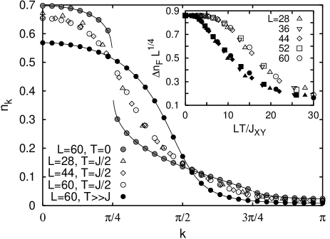
FIG. 2.: Momentum distribution of the $tJ_{XY}$ model for $T=0$ (solid line: $L=500$), $T/\tilde{J}=0.5$, and $t\gg T\gg\tilde{J}$ (solid line: $L=300$) for quarter filling ($L=2N$) and zero magnetic field. There are strong finite size effects for $T=\tilde{J}/2$. In the insert we show the scaling of $\Delta n_{F}$ for zero magnetic field (solid) and zero magnetization (empty symbols) obtained from different system sizes and temperatures.

We show our numerical results in Fig. 2. The $T=0$ result shows power law behavior at the Fermi momentum. Increasing the temperature, the power law survives until some crossover temperature ($\approx\tilde{J}/L$), where it becomes a continuous function of momentum for higher temperatures. To study this behavior in detail, we concentrate on the jump at $k_{F}$, defined as $\Delta n_{F}=n_{k^{-}_{F}}-n_{k^{+}_{F}}$, where $k^{\pm}_{F}=k_{F}\pm\pi N/L$ are the momenta of the finite system closest to the Fermi point. This jump is finite for finite size system and scales with $L^{-\alpha}$ in the Luttinger-liquid. If the singularity disappears and $n_{k}$ becomes a continuous function around $k_{F}$, then $\Delta n_{F}\propto 1/L$. In the inset of Fig. 2 we show the “size independent” $L^{\alpha}\Delta n_{F}$ vs. $LT/\tilde{J}$. It is remarkable, that at low temperature the points follow a universal curve:

$\displaystyle\Delta n_{F}=L^{-\alpha}f(LT/\tilde{J}).$

A crossover temperature, scaling with $\tilde{J}/L$, can be clearly observed, and for larger temperatures $L^{\alpha}\Delta n_{F}\rightarrow 0$. This behavior can be understood if we recall that the temperature enters by dividing the energy $\propto 2\pi u_{\sigma}/L$ of the low-energy excitations.

c Local spectral function:

The single-particle density of states is given by

$$B(\omega)=\sum_{Q,\sigma}D_{\sigma}(Q,\beta)B_{Q}(\omega),$$ (15)

where $B_{Q}(\omega)=\frac{1}{L}\sum_{k}B_{Q}(k,\omega)$. Let us concentrate on the isotropic $tJ$ model (equivalent to large-$U$ Hubbard model) in the limiting $T=0$ and $t\gg T\gg\tilde{J}$ cases only. At low temperatures $D_{\sigma}(Q,\beta)$ is large near $Q=\pi/2$, and the largest part in the convolution (15) comes from $B_{Q=\pi/2}(\omega)$. For the “hot spin” case, $D_{\sigma}(Q,\beta)$ is large near $Q=\pi$, and $B_{Q=\pi}(\omega)$ gives most of the contribution to $B(\omega)$, shown in Fig. 3. In other words, increasing the temperature we transfer less and less momentum to the spins, and the role of the orthogonality catastrophe in $B_{Q}(\omega)$ decreases. Since changing $Q$ results in a considerable redistribution of the weight in $B_{Q}(\omega)$ (see the inset in Fig. 3), the weight transfer of $B(\omega)$ at the energy scale of $t$ is due to the temperature dependence of $D_{\sigma}(Q,\beta)$ set on a much smaller temperature scale – naively we would expect smearing of $B(\omega)$ near the Fermi energy within $|\omega-\varepsilon_{F}|\approx T$. We should also note that the divergence of the spectral function at the Fermi energy is purely the artifact of the $J/t\rightarrow 0$ limit[19]. For finite $J$, the local spectral function has a broad peak around $\omega\approx\frac{\pi}{2}\tilde{J}$ due to the spinon dispersion, and a second broad peak near the band edge ($\omega\approx 2\tilde{t}$). The weight transfer then would be from the“spinon” to the “holon” peak. A similar weight redistribution is observed in the two-dimensional $tJ$ model as well.[23]

FIG. 3.: Local spectral function for $T=0$ (solid) and $t\gg T\gg\tilde{J}$ (dashed line) for the quarter-filled Hubbard model, $L=220$. For this particular filling $\varepsilon_{F}=0$. In the inset: $B_{Q}(\omega)$ for different values of $Q$.

To conclude, we have studied the temperature evolution of the momentum distribution function and local spectral function. First, we give a method to calculate $n_{k}$ for large system sizes for the $tJ_{XY}$ model at zero temperature. Next, we observed that the power-law behavior is restricted to temperatures inversely proportional to the system size. In the thermodynamic limit the system is critical at $T=0$ only. Finally, a weight redistribution in the single-particle density of states takes place over a broad energy range, which can be easily understood using the concept of “spin-charge” separation.

We would like to thank H. Frahm, J. Jaklič, H. Shiba and W. Stephan for stimulating discussions.

REFERENCES

[1]
[2]
On leave from Research Institute for Solid State Physics,
Budapest, Hungary.
[3]
J. Sólyom, Adv. Phys. 28, 201 (1979).
[4]
I. E. Dzyaloshinkii and A. I. Larkin, Sov. Phys. JETP 38, 202 (1974).
[5]
J. Voit, Rep. Prog. Phys. 58, 977 (1995) and references therein.
[6]
F. D. M. Haldane, J. Phys. C 14, 2585 (1981).
[7]
H. J. Schulz, Phys. Rev. Lett. 64, 2831 (1990).
[8]
H. Frahm and V. E. Korepin, Phys. Rev. B 42, 10553 (1990);
N. Kawakami and S. K. Yang, Phys. Lett. A 148, 359 (1990).
[9]
B. Dardel et al, Europhys. Lett. 24, 687 (1993);
C. Coluzza et al., Phys. Rev. B 47, 6625 (1993);
M. Nakamura et al., Phys. Rev. B 49, 16191 (1994);
T. Takahashi et al., Phys. Rev. B 53, 1790 (1996).
[10]
C. Kim et al., Phys. Rev. Lett. 77, 4054 (1996).
[11]
A. B. Harris and R. V. Lange, Phys. Rev. 157, 295 (1967).
[12]
E. Dagotto, Rev. Mod. Phys. 66, 763 (1994).
[13]
R. Preuss et al., Phys. Rev. Lett. 73, 732 (1994);
M. Imada and Y. Hatsugai, J. Phys. Soc. Jpn. 58, 3752 (1989).
[14]
F. Woynarovich, J. Phys. C 15, 85 (1982).
[15]
M. Ogata and H. Shiba, Phys. Rev. B 41, 2326 (1990).
[16] S. Eggert, H. Johannesson, and A. Mattsson,
Phys. Rev. Lett. 75, 1505 (1996);
M. Fabrizio and A. O. Gogolin, Phys. Rev. B 51, 7827 (1995).
[17]
T. Pruschke and H. Shiba, Phys. Rev. B 44, 205 (1991).
[18]
Y. Hatsugai, M.Kohmoto, T. Koma and Y. S. Wu,
Phys. Rev. B 54, 5358 (1996).
[19]
K. Penc, F. Mila and H. Shiba,
Phys. Rev. Lett. 75, 894 (1995);
K. Penc, K. Hallberg, F. Mila, H. Shiba, ibid. 77, 1390 (1996);
Phys. Rev. B. 55, Jun. 15 (1997) (cond-mat/9701051).
[20]
P. W. Anderson, Phys. Rev. Lett. 18, 1049 (1967).
[21]
S. Sorella and A. Parola, J. Phys. Condens. Matter 4, 3589 (1992).
[22]
F. Gebhard et al., Phil. Mag. B 75, 13 (1997).
[23] J. Jaklič and P. Prelovšek,
Phys. Rev. B 55, 7307 (1997).