Frictional Coulomb drag in strong magnetic fields

Abstract

A treatment of frictional Coulomb drag between two 2-dimensional electron layers in a strong perpendicular magnetic field, within the independent electron picture, is presented. Assuming fully resolved Landau levels, the linear response theory expression for the transresistivity $\rho_{21}$ is evaluated using diagrammatic techniques. The transresistivity is given by an integral over energy and momentum transfer weighted by the product of the screened interlayer interaction and the phase-space for scattering events. We demonstrate, by a numerical analysis of the transresistivity, that for well-resolved Landau levels the interplay between these two factors leads to characteristic features in both the magnetic field- and the temperature dependence of $\rho_{21}$. Numerical results are compared with recent experiments.

I Introduction

When two 2-dimensional charged systems are placed in close proximity, transport in one layer will drive the adjacent layer out of equilibrium. Even if the barrier separating the two layers is high and wide enough to prevent tunneling, interlayer interactions can still be sufficiently strong that a current drawn in one layer can drag along a current in the other layer. This phenomenon was theoretically proposed by Pogrebinskii[1] and by Price, [2] and has become known as frictional drag. In most frictional drag experiments a current ${\bf J}_{1}$ is drawn in one layer; the second layer is an open circuit and no current is allowed to flow. To oppose the dragging force, an electric field ${\bf E}_{2}$ develops in the second layer. The ratio of ${\bf E}_{2}$ and ${\bf J}_{1}$ is called the transresistivity $\rho_{21}$ [see Eq. (1) below] and is a measure of a rate of momentum transfer from the first to the second layer.

Experimental realizations of frictional drag between 2–dimensional systems were first reported by Gramila et al. for two electron layers,[3] and by Sivan et al. for electron–hole systems.[4] These experiments inspired a large number of theoretical works, and the experiments (which were all done in zero magnetic field) are by now fairly well understood.[5, 6, 7, 8, 9, 10, 11, 12]

Recently, attention has turned towards frictional drag in the presence of a magnetic field — the topic of the present paper. Experiments of drag in a magnetic field have been reported by Hill et al.,[13] Rubel et al.,[14] Feng et al.,[15] and Eisenstein et al.[16]

Frictional drag is of fundamental interest because it can serve as a sensitive probe of two important aspects of transport in mesoscopic systems, namely the screened interlayer interaction and the form of the irreducible polarization function $\chi(q,\omega)$, which is central to many theoretical considerations. In the presence of a magnetic field, in particular, the screening of the interaction and the polarization function can assume different forms depending on the number of filled Landau levels and the degree of disorder.

Over the past two decades new and often surprising aspects of the physics of 2-dimensional electron gases (2DEGs) in magnetic fields have continued to emerge.[17] Not only single layer systems show intriguing physics; double-layer quantum Hall systems also exhibit a number of interesting aspects,[18] and frictional drag is expected to do the same.

In this paper we present a treatment of Frictional Coulomb drag in strong magnetic fields where the Landau levels are fully resolved, i.e., $\omega_{c}\tau\gg 1$ where $\omega_{c}=eB/m^{*}$ is the cyclotron frequency and $\tau$ is the transport scattering time. Some numerical aspects of our work have been presented in a previous publication,[19] here we give the full details of the analytic background underlying these results, extend them to other parameter values, and compare them critically with recent experiments.[13, 14]

We work under the assumption that an independent electron picture applies. At sufficiently low temperatures and/or high magnetic fields this condition will not be satisfied and additional physics must be included as the following two examples reveal.

In disordered systems localization becomes important at low temperatures. Chalker and Daniell [20] found that the diffusion of electrons in the lowest Landau level is anomalous, i.e. the ‘diffusion constant’ scales as $D(q,\omega)=D_{0}(\omega/q^{2})^{\eta/2}$, where $\eta$ is found numerically to be $\eta\simeq 0.38$. Shimshoni and Sondhi pointed out that frictional drag would be a way to experimentally measure $\eta$, since the drag effect in that case would be proportional to $T^{2-\eta}$ at the lowest temperatures.[21] Another example consists of high mobility systems in high magnetic fields, where intralayer electron–electron interactions are important at low temperatures. At filling factor $\nu=1/2$ the 2DEG can be discussed in terms of composite fermions. The polarization function $\chi(q,\omega)$ assumes a unique form which was first derived by Halperin, Lee and Read.[22] Three recent papers[23] have considered frictional drag in this regime and shown that the transresistivity should be proportional to $T^{4/3}$ as the temperature $T$ approaches zero.

The outline of the paper is as follows. In Section II we define the model of the system and establish the theoretical framework. The transresistivity is in general given in terms of three-body correlation functions which are considered in Section III. In Section IV we examine in which limits the three-body correlation functions are proportional to the imaginary part of the polarization function. This relation has been tacitly assumed by most other authors. We discuss the result and the relation to similar results in zero magnetic field and a brief discussion of Hall-drag is provided. Numerical evaluations are presented in Section V; we focus on the dependence of the transresistivity upon magnetic field strength and temperature. Section VI summarizes the conclusions.

II Formalism

We consider a system of two 2-dimensional electron gases separated by a distance $d$. A uniform, constant magnetic field ${\mathbf{B}}=B{\mathbf{\hat{}}{z}}$ is applied perpendicular to the two layers which define the $xy$-plane. The two layers have electron densities of $n_{1}$ and $n_{2}$, respectively. When a current density ${\mathbf{J}}_{1}$ is drawn in layer 1, the interlayer interactions will induce an electric field ${\mathbf{E}}_{2}$ in layer 2, which is an open circuit (i.e., no current is allowed to flow in layer 2). The induced electric field can be measured by a voltage probe, and the transresistivity tensor is defined according to

$${\mathbf{E}}_{2}=\tensor{\rho}_{21}{\mathbf{J}}_{1}.$$ (1)

The transresistivity is what is measured experimentally and hence the object to determine. However, linear response theory, on which our theoretical approach is based, yields the transconductivity $\tensor{\sigma}_{21}$, defined by an experiment where the first layer is biased with an electric field and the induced current density is measured in the second layer: ${\mathbf{J}}_{2}=\tensor{\sigma}_{21}{\mathbf{E}}_{1}$. The transresistivity can be obtained from the transconductivity by

$$\tensor{\rho}_{21} = \left[-\tensor{\sigma}_{11}\tensor{\sigma}_{21}^{-1}\tensor{\sigma}_{22}+\tensor{\sigma}_{12}\right]^{-1}$$ (2)

$$\simeq -\tensor{\rho}_{22}\tensor{\sigma}_{21}\tensor{\rho}_{11},$$ (3)

where the approximate equality is valid because we assume the magnitude of the individual layer conductivities, $(\tensor{\rho}_{11})^{-1}$ and $(\tensor{\rho}_{22})^{-1}$, to be much larger than the transconductivity.

To calculate the transconductivity we follow the general framework developed independently by Kamenev and Oreg,[24] and by Flensberg, Hu, Jauho and Kinaret.[25] The transconductivity is calculated using the Kubo formula for linear response,[26] i.e., it is expressed as a current–current correlation function

$$\sigma_{21}^{\alpha\gamma}({\mathbf{k}},\Omega)=\frac{ie^{2}}{\hbar\Omega}\Pi_{21}^{\alpha\gamma,r}({\mathbf{k}},\Omega),$$ (4)

where $\Pi_{21}^{\alpha\gamma,r}({\mathbf{k}},\Omega)$ is the Fourier transform of the retarded current–current correlation function

$$\Pi_{21}^{\alpha\gamma,r}({\mathbf{x}}-{\mathbf{x}^{\prime}},t-t^{\prime})=-i\theta(t-t^{\prime})\langle[j_{2}^{\alpha}({\mathbf{x}},t)\ ,\ j_{1}^{\gamma}({\mathbf{x}^{\prime}},t^{\prime})]\rangle.$$ (5)

Here ${\bf j}_{1}$ and ${\bf j}_{2}$ are (kinematic) particle current operators in the two different layers (denoted by the subscripts 1 and 2), and $\alpha$ and $\gamma$ are Cartesian coordinates of the two-by-two transconductivity tensor. $\langle\cdots\rangle$ is a statistical average and $[\cdots,\cdots]$ is a commutator. The position vectors ${\mathbf{x}}$ and ${\mathbf{x}^{\prime}}$ reside in the 2-dimensional planes of the 2DEGs. In this paper, we assume like charges in the two layers; the sign of $\sigma_{21}$ is reversed for unlike charges.

To lowest order in the screened interlayer interaction, the transconductivity can be expressed as[24, 25]

$$\sigma_{21}^{\alpha\gamma} = \frac{e^{2}}{2\hbar^{3}A}\sum_{{\mathbf{q}}}\int\frac{d\omega}{2\pi}\left|\frac{V_{21}(q)}{{\mathcal{E}}(q,\omega)}\right|^{2}\left(-\frac{\partial n_{B}(\omega)}{\partial\omega}\right)$$ (7)

$$\times\Delta_{2}^{\alpha}({\mathbf{q}},{\mathbf{q}},\omega+i\eta,\omega-i\eta)\Delta_{1}^{\gamma}(-{\mathbf{q}},-{\mathbf{q}},-\omega-i\eta,-\omega+i\eta),$$

where $\eta$ is a positive infinitesimal, $A$ is a normalization area, $V_{21}(q)$ is the interlayer Coulomb interaction, ${\mathcal{E}}(q,\omega)$ is the screening function, and $n_{B}$ is the Bose–Einstein distribution function. Notice that the transconductivity tensor is a dyadic product of the two three-body correlation functions ${\mathbf{\Delta}}_{2}$ and ${\mathbf{\Delta}}_{1}$, which are defined by

$$\Delta_{i}^{\alpha}({\mathbf{x}},\tau;{\mathbf{x}^{\prime}},\tau^{\prime};{\mathbf{x}^{\prime\prime}},\tau^{\prime\prime})=-\langle T_{\tau}\left\{j_{i}^{\alpha}({\mathbf{x}},\tau)\rho_{i}({\mathbf{x}^{\prime}},\tau^{\prime})\rho_{i}({\mathbf{x}^{\prime\prime}},\tau^{\prime\prime})\right\}\rangle,$$ (8)

and will be referred to as the triangle functions. The following convention for the Fourier transform has been adopted

$$\Delta_{i}^{\alpha}({\mathbf{x}},\tau;{\mathbf{x}^{\prime}},\tau^{\prime};{\mathbf{x}^{\prime\prime}},\tau^{\prime\prime})=\frac{1}{A^{2}}\sum_{{\mathbf{q}_{1}},{\mathbf{q}_{2}}}\frac{1}{(\hbar\beta)^{2}}\sum_{i\omega_{1},i\omega_{2}} e^{i{\mathbf{q}_{1}}\cdot({\mathbf{x}}-{\mathbf{x}^{\prime\prime}})+i{\mathbf{q}_{2}}\cdot({\mathbf{x}^{\prime}}-{\mathbf{x}^{\prime\prime}})}e^{-i\omega_{1}(\tau-\tau^{\prime\prime})-i\omega_{2}(\tau^{\prime}-\tau^{\prime\prime})}$$ (10)

$$\times\Delta_{i}^{\alpha}({\mathbf{q}_{1}}+{\mathbf{q}_{2}},{\mathbf{q}_{2}},i\omega_{1}+i\omega_{2},i\omega_{2}).$$

This Fourier transform convention relies on the translational invariance of the triangle function which applies when we consider infinite systems; extra caution should be exercised when considering systems of finite extent.

III The triangle function

After the expansion in the interlayer interaction the correlation functions ${\mathbf{\Delta}}_{1}$ and ${\mathbf{\Delta}}_{2}$ only depend on the individual layers and contain all microscopic details of these. To proceed we must choose a model for the individual layers.

The non-interacting electron model is a good approximation for the experimental systems studied so far[3, 4, 13, 14] as long as the magnetic field is not too strong and the temperature not too low (see Introduction). Hence, we shall treat the individual layers as non-interacting electrons scattering against random impurities. Within this model it has been shown that for short range impurity potentials,[24, 25] the triangle function is proportional to the imaginary part of the polarization function

$${\mathbf{\Delta}}(\pm{\mathbf{q}},\pm{\mathbf{q}},\pm(\omega+i\eta),\pm(\omega-i\eta))=\frac{2\tau\hbar^{2}}{m^{*}}\ {\mathbf{q}}\ {\mathrm{I}m}\chi(q,\omega)$$ (11)

in absence of a magnetic field. [The same form is recovered if electron-electron scattering keeps the distribution function as a shifted Fermi-Dirac.[9]] Here $m^{*}$ is the effective electron mass, and the transport scattering time $\tau$ is assumed to be energy independent. In the following two sections it will be shown that we can obtain a similar relation in the limit of $\omega_{c}\tau\gg 1$ for short ranged scattering potentials.

Up to this point an ensemble average over impurity configurations has been implicitly understood. When the triangle function is expressed in terms of Green functions, the impurity averaging is accounted for by dressing the Green functions by self-energies and including vertex functions where they connect. A careful account of impurities is necessary in the presence of a magnetic field because of the high Landau level degeneracy; leaving out impurities would lead to unphysical divergences.

The free Hamiltonian is

$$H=\frac{1}{2m^{*}}\left({\mathbf{p}}+e{\mathbf{A}}\right)^{2}$$ (12)

with ${\mathbf{B}}={\mathbf{\nabla}}\times{\mathbf{A}}$. We choose to work in the Landau gauge, ${\mathbf{A}}=(0,Bx,0)$, so that each eigenstate is characterized by two quantum numbers: $|N\rangle=|n,k\rangle$. For infinite systems, the eigenenergies only depend on the Landau level index $n$: $\varepsilon_{n}=(n+1/2)\hbar\omega_{c}$.

In terms of creation and annihilation operators, the density operator is

$$\rho({\mathbf{x}^{\prime}},\tau)=\frac{1}{A}\sum_{{\mathbf{q}},N,M}e^{i{\mathbf{q}}\cdot{\mathbf{x}^{\prime}}}\langle N|e^{i{\mathbf{q}}\cdot{\mathbf{r}}}|M\rangle c_{N}^{\dagger}(\tau)c_{M}(\tau)$$ (13)

and the operator for the current is given by

$${\mathbf{j}}(\tau)=\frac{\ell\omega_{c}}{A}\sum_{N}\left({\mathbf{w}}_{1}\sqrt{n+1}c_{N+1}^{\dagger}(\tau)c_{N}(\tau)+{\mathbf{w}}_{2}\sqrt{n}c_{N-1}^{\dagger}(\tau)c_{N}(\tau)\right),$$ (14)

where we have defined the two vectors, ${\mathbf{w}}_{1}=i\hat{{\mathbf{x}}}+\hat{{\mathbf{y}}}$ and ${\mathbf{w}}_{2}={\mathbf{w}}_{1}^{*}=-i\hat{{\mathbf{x}}}+\hat{{\mathbf{y}}}$ with $\hat{{\mathbf{x}}}$ and $\hat{{\mathbf{y}}}$ being unit vectors defining the planes of the electron layers. When the density and current operators are inserted in the expression for the triangle function, we get terms involving the statistical average of products of 3 creation and 3 annihilation operators. The Hamiltonian for impurity scattering is quadratic in creation and annihilation operators, which means that we can use Wick’s theorem to write the product of creation and annihilation operators in terms of products of 3 Green functions. Inserting (13) and (14) in Eq. (8) we get two connected diagrams. One of these is given by (see Fig. 1)

$$\frac{-1}{A^{3}}\sum_{N,N^{\prime},M,{\bf q}} e^{i{\bf q}\cdot({\bf x^{\prime}}-{\bf x^{\prime\prime}})}\Gamma({\bf q},N,M,\tau-\tau^{\prime},\tau^{\prime}-\tau^{\prime\prime})G(N,\tau-\tau^{\prime})$$ (17)

$$\gamma^{\alpha}({\bf Q}=0,N^{\prime},N,\tau^{\prime\prime}-\tau,\tau-\tau^{\prime})G(N^{\prime},\tau^{\prime\prime}-\tau)$$

$$\Gamma(-{\bf q},M,N^{\prime},\tau^{\prime}-\tau^{\prime\prime},\tau^{\prime\prime}-\tau)G(M,\tau^{\prime}-\tau^{\prime\prime})$$

where a current vertex $\gamma$ and charge vertices $\Gamma$ have been included to take account of impurity scattering; in the other diagram the direction of the arrows is reversed. The scattering of electrons against impurities is evaluated in the self-consistent Born approximation. The self-energy diagram is shown in Fig. 2a. In the limit of $\omega_{c}\tau\gg 1$ Ando and Uemura[27] have shown that the self-energy is given by

$$\hbar\Sigma^{r,a}(n,\epsilon)=\frac{\hbar\epsilon-\varepsilon_{n}}{2}-\frac{\Gamma_{0}}{2}\sqrt{\left(\frac{\hbar\epsilon-\varepsilon_{n}}{\Gamma_{0}}\right)^{2}-1}$$ (18)

where $\Gamma_{0}^{2}=(2/\pi)\hbar\omega_{c}(\hbar/\tau)$, $\tau$ being the transport scattering time at zero magnetic field. The imaginary part of Eq. (18) is taken as negative (positive) for the retarded (advanced) function. The width of the Landau level, $2\Gamma_{0}$, is independent of the Landau level index if the range of the scattering potential is smaller than the magnetic length. The choice of self-energy diagram implies, by a Ward identity, a specific choice of vertex functions. Born approximation for the self-energy implies that we must sum ladder diagrams for the vertex functions. In the limit of short range scattering potential the contribution from the ladder sum to the current vertex function can be neglected,[27] i.e. $\gamma$ can be approximated by a bare current vertex and hence $N^{\prime}=N\pm 1$ in Eq. (17). For the charge vertex, on the other hand, the ladder sum is important. Fig. 2b shows the diagrams corresponding to the following integral equation for $\Gamma$:

$$\Gamma({\mathbf{q}},n,m,i\epsilon_{1},i\epsilon_{2}) = f_{n,m}({\mathbf{q}})+\frac{\rho_{{\mathrm{i}mp}}}{\hbar^{2}}\sum_{a,b}\int\!\frac{d{\mathbf{k}}}{(2\pi)^{2}}U^{2}(k)f_{b,m}({\mathbf{k}})f_{n,a}(-{\mathbf{k}})$$ (20)

$$\times{\mathcal{G}}(a,i\epsilon_{1}){\mathcal{G}}(b,i\epsilon_{2})e^{i\ell^{2}(k_{x}q_{y}-k_{y}q_{x})}\Gamma({\mathbf{q}},a,b,i\epsilon_{1},i\epsilon_{2}),$$

where $\rho_{{\mathrm{i}mp}}$ is the density of impurities, $U(k)$ is the impurity potential, and ${\mathcal{G}}$ is a Matsubara Green function. The bare charge vertex is given by

$$f_{n,m}({\mathbf{q}})=\left\{\begin{array}[]{ll}e^{-(\ell q/2)^{2}}\sqrt{\frac{m!}{n!}2^{m-n}}\left(-\ell(iq_{x}+q_{y})\right)^{n-m}L_{m}^{n-m}((\ell q)^{2}/2)&\ \ ,m\leq n\\ e^{-(\ell q/2)^{2}}\sqrt{\frac{n!}{m!}2^{n-m}}\left(-\ell(iq_{x}-q_{y})\right)^{m-n}L_{n}^{m-n}((\ell q)^{2}/2)&\ \ ,n\leq m\end{array}\right.$$ (21)

where $L_{n}^{m}$ are the Laguerre polynomials and $\ell=\sqrt{\hbar/eB}$ is the magnetic length.

In terms of dressed Matsubara Green functions and vertex functions, the expression for the triangle function is

$${\mathbf{\Delta}}({\mathbf{q}},{\mathbf{q}},i\Omega+i\omega,i\omega)=\frac{-\omega_{c}}{2\pi\ell\hbar\beta}\sum_{n,m,i\omega_{1}}\sqrt{n}\left({\mathbf{w}}_{1}{\mathcal{F}}_{1}+{\mathbf{w}}_{2}{\mathcal{F}}_{2}\right)\;,$$ (22)

where

$${\mathcal{F}}_{1} = \Gamma({\mathbf{q}},n-1,m,i\omega_{1},i\omega_{1}+i\omega)\Gamma(-{\mathbf{q}},m,n,i\omega_{1}+i\omega,i\omega_{1}-i\Omega)$$ (23)

$$\times {\mathcal{G}}(n,i\omega_{1}-i\Omega){\mathcal{G}}(m,i\omega_{1}+i\omega){\mathcal{G}}(n-1,i\omega_{1})$$ (24)

$$+ \Gamma({\mathbf{q}},m,n,i\omega_{1}-i\omega,i\omega_{1})\Gamma(-{\mathbf{q}},n-1,m,i\omega_{1}+i\Omega,i\omega_{1}-i\omega)$$ (25)

$$\times {\mathcal{G}}(n,i\omega_{1}){\mathcal{G}}(m,i\omega_{1}-i\omega){\mathcal{G}}(n-1,i\omega_{1}+i\Omega)$$ (26)

and

$${\mathcal{F}}_{2} = \Gamma({\mathbf{q}},n,m,i\omega_{1},i\omega_{1}+i\omega)\Gamma(-{\mathbf{q}},m,n-1,i\omega_{1}+i\omega,i\omega_{1}-i\Omega)$$ (27)

$$\times {\mathcal{G}}(n,i\omega_{1}){\mathcal{G}}(m,i\omega_{1}+i\omega){\mathcal{G}}(n-1,i\omega_{1}-i\Omega)$$ (28)

$$+ \Gamma({\mathbf{q}},m,n-1,i\omega_{1}-i\omega,i\omega_{1})\Gamma(-{\mathbf{q}},n,m,i\omega_{1}+i\Omega,i\omega_{1}-i\omega)$$ (29)

$$\times {\mathcal{G}}(n,i\omega_{1}+i\Omega){\mathcal{G}}(m,i\omega_{1}-i\omega){\mathcal{G}}(n-1,i\omega_{1})\;.$$ (30)

The summation over Matsubara frequencies $i\omega_{1}$ can be carried out as a contour integration. The function ${\mathbf{\Delta}}({\mathbf{q}},{\mathbf{q}},\omega+i\eta,\omega-i\eta)$ is then obtained by letting $i\Omega+i\omega\rightarrow\Omega+\omega+i\eta$, $i\Omega\rightarrow\Omega+i\eta$, and $i\omega\rightarrow\omega-i\eta$.[25] In the static limit, $\Omega\rightarrow 0$, the result is

$${\mathbf{\Delta}}({\mathbf{q}},{\mathbf{q}},\omega+i\eta,\omega-i\eta) = \frac{\hbar\omega_{c}}{2\pi\ell}\sum_{n,m}\sqrt{n}\int\frac{d\epsilon}{2\pi i}n_{F}(\epsilon)$$ (33)

$$\times\Big{[}{\mathbf{w}}_{1}\Big{(}P({\mathbf{q}},n,m,\epsilon,\epsilon+\omega)+P(-{\mathbf{q}},n,m,\epsilon,\epsilon-\omega)\Big{)}$$

$$\ \ \ -{\mathbf{w}}_{2}\Big{(}P^{*}({\mathbf{q}},n,m,\epsilon,\epsilon+\omega)+P^{*}(-{\mathbf{q}},n,m,\epsilon,\epsilon-\omega)\Big{)}\Big{]}$$

with

$$P ({\mathbf{q}},n,m,\epsilon,\epsilon+\omega)=$$ (40)

$$\Gamma^{+-}({\mathbf{q}},n,m,\epsilon,\epsilon+\omega)\Gamma^{--}(-{\mathbf{q}},m,n-1,\epsilon+\omega,\epsilon)G^{r}(n,\epsilon)G^{a}(m,\epsilon+\omega)G^{a}(n-1,\epsilon)$$

$$-\Gamma^{--}({\mathbf{q}},n,m,\epsilon,\epsilon+\omega)\Gamma^{--}(-{\mathbf{q}},m,n-1,\epsilon+\omega,\epsilon)G^{a}(n,\epsilon)G^{a}(m,\epsilon+\omega)G^{a}(n-1,\epsilon)$$

$$+\Gamma^{++}({\mathbf{q}},n,m,\epsilon-\omega,\epsilon)\Gamma^{+-}(-{\mathbf{q}},m,n-1,\epsilon,\epsilon-\omega)G^{r}(n,\epsilon-\omega)G^{r}(m,\epsilon)G^{a}(n-1,\epsilon-\omega)$$

$$-\Gamma^{+-}({\mathbf{q}},n,m,\epsilon-\omega,\epsilon)\Gamma^{--}(-{\mathbf{q}},m,n-1,\epsilon,\epsilon-\omega)G^{r}(n,\epsilon-\omega)G^{a}(m,\epsilon)G^{a}(n-1,\epsilon-\omega)$$

$$+\Gamma^{++}({\mathbf{q}},n,m,\epsilon,\epsilon+\omega)\Gamma^{++}(-{\mathbf{q}},m,n-1,\epsilon+\omega,\epsilon)G^{r}(n,\epsilon)G^{r}(m,\epsilon+\omega)G^{r}(n-1,\epsilon)$$

$$-\Gamma^{++}({\mathbf{q}},n,m,\epsilon,\epsilon+\omega)\Gamma^{+-}(-{\mathbf{q}},m,n-1,\epsilon+\omega,\epsilon)G^{r}(n,\epsilon)G^{r}(m,\epsilon+\omega)G^{a}(n-1,\epsilon).$$

The plus and minus signs attached to the vertex functions indicate the signs of the imaginary infinitesimals that should be added to the frequency arguments. From (33) it can be realized that ${\mathbf{\Delta}}$ is a vector with purely real components. Other general properties of ${\bf\Delta}$ are given in Appendix A.

IV Triangles to bubbles

We now show that in the limit of short range scattering potentials and for $\omega_{c}\tau\gg 1$, we can express the triangle function in terms ${\mathbf{q}}$ and the imaginary part of the proper polarization function.

The proper polarization function is obtained by analytical continuation of the density–density correlation function shown in Fig. 3. From the structure it is seen, that it involves two Green functions $G$, one bare vertex $f$, and one vertex function $\Gamma$; symbolically $\chi\sim f\,G\,G\,\Gamma$. The triangle function, on the other hand, involves products of three Green functions and two vertex functions; symbolically $\Delta\sim G\,G\,G\,\Gamma\,\Gamma$. To reduce the triangle function to the polarization function we must therefore reduce three Green functions to two, and two vertex functions to one vertex function and a bare vertex. Furthermore we must introduce a factor of ${\mathbf{q}}$ if we want an expression similar to Eq. (11). Symbolically the task is to do the simplification: $G\,G\,G\,\Gamma\,\Gamma\longrightarrow{\mathbf{q}}\,G\,G\,\Gamma\,f$, which we shall now proceed to carry out.

The key to the problem is to notice that in the expression (40) two of the Green functions and both the vertex functions in the product $G\,G\,G\,\Gamma\,\Gamma$ have neighboring Landau level indices, $n$ and $n-1$. The retarded and advanced Green functions are given by $G^{r,a}(n,\epsilon)=[\epsilon-\frac{1}{\hbar}\varepsilon_{n}-\Sigma^{r,a}(n,\epsilon)]^{-1}$. Using the identity $1/AB=(1/A-1/B)/(B-A)$ we get

$$G^{r}(n,\epsilon)G^{a}(n-1,\epsilon)=\frac{G^{r}(n,\epsilon)-G^{a}(n-1,\epsilon)}{\omega_{c}+\Sigma^{r}(n,\epsilon)-\Sigma^{a}(n-1,\epsilon)}.$$ (41)

In the limit $\omega_{c}\tau\gg 1$ the self-energies can be neglected compared to the cyclotron frequency, and we can approximate

$$G^{r}(n,\epsilon)G^{a}(n-1,\epsilon)\simeq\frac{G^{r}(n,\epsilon)-G^{a}(n-1,\epsilon)}{\omega_{c}}.$$ (42)

We have thus reduced products of three Green functions to products of two Green functions.

To reduce the product of two vertex functions to one vertex function and one bare vertex is more involved and therefore deferred to Appendix B where it is shown that we can do the approximation in leading order of $(\omega_{c}\tau)^{-1}$

$$\Gamma^{+-} ({\mathbf{q}},n,m,\epsilon,\epsilon+\omega)\Gamma^{--}(-{\mathbf{q}},m,n-1,\epsilon+\omega,\epsilon)G^{r}(n,\epsilon)G^{a}(m,\epsilon+\omega)G^{a}(n-1,\epsilon)$$ (45)

$$\simeq\frac{1}{\omega_{c}}\Gamma^{+-}({\mathbf{q}},n,m,\epsilon,\epsilon+\omega)f_{m,n-1}(-{\mathbf{q}})G^{r}(n,\epsilon)G^{a}(m,\epsilon+\omega)$$

$$\ \ -\frac{1}{\omega_{c}}f_{n,m}({\mathbf{q}})\Gamma^{--}(-{\mathbf{q}},m,n-1,\epsilon+\omega,\epsilon)G^{a}(m,\epsilon+\omega)G^{a}(n-1,\epsilon).$$

Notice that the full vertex function with same Landau indices as the Green functions is retained, and that the signs of the infinitesimals in the vertex function naturally follow the signs of the infinitesimal on the Green functions that it is multiplying. In the above expression there seems to be a mismatch between the Landau level indices of the Green functions and the Landau level indices of the bare vertices $f_{n,m}$ multiplying them. Matching indices are recovered by the identity

$$\sqrt{n+1}f_{n+1,m}({\mathbf{q}})-\sqrt{m}f_{n,m-1}({\mathbf{q}})=\frac{-\ell(iq_{x}+q_{y})}{\sqrt{2}}f_{n,m}({\mathbf{q}}),$$ (46)

which also introduces ${\mathbf{q}}$ into the expression. The square root factors in Eq. (46) come from the bare current vertices (see Eq. (14)). With these approximations it is a matter of simple manipulations to reach the following relation

$${\mathbf{\Delta}}(\pm{\mathbf{q}},\pm{\mathbf{q}},\pm(\omega+i\eta),\pm(\omega-i\eta))=\mp\frac{2\hbar^{2}}{eB^{2}}\,{\mathbf{q}}\times{\mathbf{B}}\ {\mathrm{I}m}\chi(q,\omega),$$ (47)

which is valid for $\omega_{c}\tau\gg 1$. Note that for $B=0$, ${\mathbf{\Delta}}(\pm{\mathbf{q}},\pm{\mathbf{q}},\pm(\omega+i\eta)$ have the same sign. Here the (irreducible) polarization function is

$$\chi (q,\omega)=\frac{1}{\hbar\pi\ell^{2}}\sum_{n,m}\int\frac{d\epsilon}{2\pi i}n_{F}(\epsilon)$$ (52)

$$\times\Big{[}G^{r}(m,\epsilon+\omega)f_{n,m}({\mathbf{q}})$$

$$\ \ \ \ \ \ \ \times\left\{G^{a}(n,\epsilon)\Gamma^{+-}(-{\mathbf{q}},m,n,\epsilon+\omega,\epsilon)-G^{r}(n,\epsilon)\Gamma^{++}(-{\mathbf{q}},m,n,\epsilon+\omega,\epsilon)\right\}$$

$$\ \ \ +G^{a}(m,\epsilon-\omega)f_{m,n}({\mathbf{q}})$$

$$\ \ \ \ \ \ \ \times\left\{G^{a}(n,\epsilon)\Gamma^{--}(-{\mathbf{q}},n,m,\epsilon,\epsilon-\omega)-G^{r}(n,\epsilon)\Gamma^{+-}(-{\mathbf{q}},n,m,\epsilon,\epsilon-\omega)\right\}\Big{]}.$$

To obtain the transresistivity we must know the single–layer resistivities $\tensor{\rho_{ii}}$ [see Eq. (2)]. For isotropic systems they have the generic structure

$$\tensor{\rho_{ii}}=\rho_{0i}\left(\begin{array}[]{cc}a_{i}&b_{i}\\ -b_{i}&a_{i}\end{array}\right)$$ (53)

with $\rho_{0i}=m_{i}^{*}/(n_{i}e^{2}\tau_{i})$ being the resistivity in zero magnetic field. Combining Eqs. (2), (47) and (53) we find that for $b\gg a$ the transresistivity tensor is diagonal in cartesian coordinates; the diagonal elements given by

$$\rho_{21}^{xx}=\left[\frac{b_{1}b_{2}}{(\omega_{c}\tau)_{1}(\omega_{c}\tau)_{2}}\right]\frac{(-\hbar^{2})}{4e^{2}n_{1}n_{2}k_{B}T}\frac{1}{A}\sum_{{\mathbf{q}}}q^{2}\int\frac{d\omega}{2\pi}\left|\frac{V_{21}(q)}{{\mathcal{E}}(q,\omega)}\right|^{2}\frac{\mathrm{Im}\chi_{1}({\mathbf{q}},\omega)\mathrm{Im}\chi_{2}({\mathbf{q}},\omega)}{\sinh^{2}(\hbar\omega/2k_{B}T)},$$ (54)

A semiclassical treatment of $\tensor{\rho}_{ii}$ yields $b_{i}=(\omega_{c}\tau)_{i}$, so that the term in the square bracket above is unity. We assume this to be the case in our numerical evaluations. As the quantum Hall regime is approached, $b_{i}/(\omega_{c}\tau)_{i}$ starts deviating from 1; however this deviation does not change the main features of the numerical results presented in Sec. V.

A A conjecture: generalization to arbitrary $B$-field

In the previous subsection it was shown, that when the individual layers are treated as non-interacting electrons scattering against short-range impurities, the triangle function is related to the imaginary part of the polarization function in the limit of $\omega_{c}\tau\gg 1$. Work has also been done in the small magnetic field limit $\omega_{c}\tau\ll 1$.[24, 28] We now discuss a conjecture for the generalization of the expression for ${\bf\Delta}$ for arbitrary magnetic field strengths which extrapolates between the weak and strong field limits.

For zero magnetic field the triangle function is proportional to the imaginary part of the polarization function when the impurity scattering time is independent of energy (see Eq. (11)).[25] One case of an energy independent transport time is when the range of the impurity potential is short compared to the Fermi wavelength. Likewise, for high magnetic fields we found that a prerequisite for a simple relation between ${\mathbf{\Delta}}$ and Im$\chi$ is short ranged scatterers. The task in this section is to bridge the gap between zero and high magnetic field. In order to do this we first observe that only two vectors can be constructed in the $xy$-plane, namely ${\mathbf{q}}$ and ${\mathbf{q}}\times{\mathbf{B}}$. The triangle function is therefore of the form

$${\mathbf{\Delta}}(\pm{\mathbf{q}},\pm{\mathbf{q}},\pm(\omega+i\eta),\pm(\omega-i\eta))=\Delta_{\|}(q,\omega,B){\mathbf{\hat{}}{q}}\pm\Delta_{\perp}(q,\omega,B){\mathbf{\hat{}}{q}}\times{\mathbf{\hat{}}{B}}\;,$$ (55)

where the carets denote unit vectors. Knowledge of the zero and high magnetic field limits, results from a semiclassical analysis,[28] and a perturbational calculation[24] suggest the following conjecture for the form of the triangle function, valid for short range scatterers but for arbitrary magnetic field strength:

$${\mathbf{\Delta}}_{i}(\pm{\mathbf{q}},\pm{\mathbf{q}},\omega\pm i\eta,\omega\mp i\eta)=\frac{2\tau_{i}\hbar^{2}}{m^{*}_{i}}\left(\frac{1}{1+\alpha_{i}^{2}}{\mathbf{q}}\mp\frac{\alpha_{i}}{1+\alpha_{i}^{2}}{\mathbf{q}}\times{\mathbf{\hat{}}{B}}\right){\mathrm{I}m}\chi_{i}(q,\omega,B),$$ (56)

where $\alpha_{i}(B)$ is a parameter to be determined. The magnetic field has been added as an argument of the polarization function to emphasize that it should be evaluated in the presence of the magnetic field.

The $\alpha_{i}(B)$ should be chosen so that Eq. (56) is consistent with known results. One such empirical result is that so far no experiment has ever observed Hall drag.[29] If one assumes that Hall drag is absent (i.e., $\rho_{21}^{xy}=0$), then

$$\alpha_{i}=\frac{b_{i}}{a_{i}}.$$ (57)

With the above choice one obtains in the low-field Drude limit $\alpha_{i}=(\omega_{c}\tau)_{i}$, which is consistent with semiclassical low-field results.[28] Furthermore, we note it reproduces the result obtained using the memory-functional formalism of Ref. [7].

We can illustrate the plausibility of a vanishing Hall-drag by a very simple argument. The electrons in layer 2 are influenced by two forces which must add up to zero because there is no current in layer 2, i.e.

$$0={\mathbf{F}}_{12}+(-e)\left({\mathbf{E}}_{2}+\langle{\mathbf{v}}_{2}\rangle\times{\mathbf{B}}\right)\;,$$ (58)

where ${\mathbf{F}}_{12}$ is the force from the electrons in layer 1, ${\mathbf{E}}_{2}$ is the induced electric field, and $\langle{\mathbf{v}}_{2}\rangle$ is the average velocity of the electrons in layer 2. When no current is allowed to flow in layer 2, $\langle{\bf v}_{2}\rangle=0$. Furthermore, since the Coulomb force is radial, ${\mathbf{F}}_{12}$ must be parallel to ${\mathbf{J}}_{1}$ and hence the measured electric field is parallel to the driving current, i.e. no Hall drag.

However, the above argument is not as general as it seems,[28] and to second-order in the screened interlayer interaction, Hall-drag can occur in cases where the band-structure is anisotropic, which breaks in-plane inversion symmetry and when the intralayer scattering time is energy-dependent, which does not allow a simple description based on the polarization function alone.[9, 28] Furthermore, higher-order correlation effects such as those found in an electron-hole system with bound pairs[10] may lead to a finite Hall-drag even in the absence of the conditions mentioned above.

V Numerical results

The formula for the transresistivity Eq. (54) must be evaluated numerically. We focus on the dependence on magnetic field strength and temperature. As a model for the dielectric function, we adopt the random phase approximations in which

$${\mathcal{E}}(q,\omega)=[1-\chi(q,\omega)V_{11}(q)]^{2}-[\chi(q,\omega)V_{21}(q)]^{2},$$ (59)

where $V_{11}(q)$ is the intralayer- and $V_{21}(q)$ is the interlayer Coulomb interaction (we have assumed that $\chi_{1}=\chi_{2}\equiv\chi$, i.e. identical layers).

The polarization function enters both directly in the Eq. (54) and indirectly through the dielectric function. The general expression for $\chi(q,\omega)$ is given in Eq. (52). To make the numerical evaluations tractable, it is necessary to make an approximation for the vertex functions, which in general are given by the integral equation (20). In Appendix B we show that when the Landau levels are clearly resolved, we can approximate

$$\Gamma({\mathbf{q}},n,m,i\epsilon+i\omega,i\epsilon)=\frac{f_{n,m}({\mathbf{q}})}{1-(\Gamma_{0}/2\hbar)^{2}{\mathcal{I}}(q,n,m){\mathcal{G}}(n,i\epsilon+i\omega){\mathcal{G}}(m,i\epsilon)}$$ (60)

with ${\mathcal{I}}(q,n,m)$ given by Eq. (B3). This approximation is consistent with the assumptions under which we derived Eq. (54) and makes the numerical evaluation tractable.

In order to avoid unphysical jumps in the chemical potential we must improve the self-consistent Born approximation (which leads to a vanishing density of states outside the Landau bands), and we use a Gaussian the density of states derived by Gerhardts,[30]

$$g_{m,\sigma}(\varepsilon)=\frac{\sqrt{2/\pi}}{2\pi\ell^{2}\Gamma_{0}}\exp\left[-2\left(\frac{\varepsilon-\varepsilon_{m}}{\Gamma_{0}}\right)^{2}\right]$$ (61)

where $\sigma$ denotes spin. The chemical potential $\mu(B,T)$ is determined implicitly by requiring the density $n$ to be given by

$$n=\sum_{m,\sigma}\int_{0}^{\infty}\!d\varepsilon\ n_{F}(\varepsilon-\mu)g_{m,\sigma}(\varepsilon).$$ (62)

This model has a finite range of magnetic fields where the density of extended states at the Fermi energy is suppressed, simulating the effect of localized states between the Landau bands, which are needed to obtain quantum Hall plateaus with a finite width. However, the quantitative details of localization, such as the critical properties of the metal-insulator transition, are not included in this simple model.

With these approximations we evaluate the transresistivity given by Eq. (54) as a function of magnetic field and temperature. For simplicity we consider two identical electron layers of densities $n_{1}=n_{2}=3\times 10^{15}$ m^-2 corresponding to a Fermi temperature of $T_{F}\simeq 120$ K. The center–to–center distance, $d$, is chosen to be 800 Å  and the well-widths are taken to be 200 Å. The Landau level width is dependent on the transport scattering time, $\tau$, which we determine by choosing a mobility, $e\tau/m^{*}$, of 25 m²/Vs. The temperature dependence of the scattering rate – which for simplicity is neglected in what follows – will eventually lead to a violation of the requirement $\omega_{c}\tau\gg 1$, and would set the upper temperature limit of the validity of the numerical evaluations.

A Magnetic field dependence

We focus on a magnetic field regime where the Landau levels are fully resolved. For simplicity we neglect spin splitting. (Because of spin degeneracy, note that filling factor $\nu$ = odd number corresponds to a half-filled Landau level, whereas filled Landau levels have $\nu$ = even number.) Experimentally there is a large regime where doubly occupied, clearly distinguishable Landau levels can be observed. For half-filled Landau levels, the density of states $g$ is enhanced over the $B=0$ value: $g=g_{0}\sqrt{2\omega_{c}\tau/\pi}$ where $g_{0}=m^{*}/\pi\hbar^{2}$. This is due to the large degeneracy of the Landau levels and implies that there are more available states close to the Fermi energy for the electrons to scatter into. Consequently a general enhancement of the transresistivity should be expected in a magnetic field. Experimentally the transresistivity has been found to increase as the square of the magnetic field as long as the Landau levels are not resolved.[13] When the Landau levels get resolved the picture is more complicated. At even filling factors the density of states is suppressed; an excitation gap develops, and the transresistivity should vanish as a result. These two expectations are both based on considerations of the density of states, i.e. the phase-space available for the interlayer e–e scattering.

The screening of the double layer system is strongly affected by the density of states and thus also strongly dependent on the magnetic field. As the density of states at the Fermi level becomes smaller the electron layers lose their ability to screen and hence the effective interlayer interaction is enhanced.

The resulting transresistivity can qualitatively be understood as a product of the available phase-space and the effective interaction. In Fig. 4 we plot $|V_{21}(q)/{\mathcal{E}}(q,\omega)|^{2}$ and [Im$\chi(q,\omega)/\sinh(\hbar\omega/2k_{B}T)]^{2}$ as a function of filling factor together with the product of the two functions for a given $q$ and $\omega$. The maxima of the product occur at magnetic fields for which the filling factor is slightly above or below an even integer (where an integral number of Landau levels are filled).

Fig. 5 shows the transresistivity as a function of magnetic field. At odd filling factors $\rho_{21}$ is enhanced (by a factor of $\sim 100$ at $\nu=3$ depending on the temperature) over the zero field value as expected. As the magnetic field is changed from an odd filling factor towards an even, we find that the transresistivity increases before it eventually gets suppressed when the chemical potential enters the excitation gap. This unusual behavior is explained by the competition of available phase-space and effective interaction.

When comparing this theory with experiments, one faces the complication of spin splitting which is present in real systems. Thus, a double peak in an experimental $\rho_{21}$ [13, 14] may be due to two partially overlapping single-peaked structures; this is the interpretation of Ref. [13]. However, Rubel et al.[14] have shown experimentally that there is a regime of magnetic fields ($\nu=$ 6–15) where the single-layer longitudinal resistivity shows no spin splitting while the transresistivity has a clear twin-peak structure. On the other hand, their data at higher magnetic fields includes spin resolved structures that do not show the predicted double-peak structure. An improved theory, which includes spin-splitting would clearly be desirable.

B Temperature dependence

We will discuss two regimes of temperature which show interesting behavior and which yield information about the polarization function and the effective interaction.

From general properties of density-response functions[31] it follows that for $q^{-1}$ larger than the smallest relevant length scale ( = elastic mean free path for $B=0$, and $\ell$ for sufficiently large $B$) and $\omega$ smaller than the inverse scattering time, the polarization function assumes a diffusive form

$$\chi(q,\omega)=-g(\mu)\frac{Dq^{2}}{Dq^{2}-i\omega},$$ (63)

where $D$ is the diffusion constant. For high magnetic fields the magnetic length $\ell=\sqrt{\hbar/eB}$ is smaller than typical interlayer distances $d$ ($\ell=180$ Å for $B=2$ T). The dominant contribution to the $q$-integral in (Eq. 54) comes from $q\leq 1/d$, and the $\omega$-integral is dominated by contributions form $\hbar\omega\lesssim k_{B}T$. Hence, if the thermal energy is smaller than $\hbar/\tau$, the diffusive form of $\chi$ prevails and we should therefore expect $\rho_{21}\sim T^{2}\ln T$ as shown by Zheng and MacDonald.[7] Numerical evaluations showing the $T^{2}\ln T$ dependence of $\rho_{21}$ were presented in a previous publication.[19] The temperature below which the diffusive behavior prevails is given by $k_{B}T_{{\mathrm{d}iff}}\approx\hbar/\tau$ and is therefore sample specific. For our choices of parameters, we find numerically that the diffusive behavior sets in at $T=0.4$ K. The $T^{2}\ln T$ is a direct consequence of the diffusive form Eq. (63), which emerges from Eq. (52) by virtue of the use of the self-consistent Born approximation for the vertex correction $\Gamma$. As mentioned in the Introduction, other temperature dependences are conceivable depending on the filling factor, the temperature regime, and the mobility of the sample.

For temperatures higher than $T_{{\mathrm{d}iff}}$, the dominant contributions to the $\omega$–integral come from $\omega>1/\tau$. In this regime both the real and imaginary part of the polarization function are strongly frequency dependent; consequently the same is true for the effective interaction $V_{21}(q)/{\mathcal{E}}(q,\omega)$. Wu et al.[32] have studied the collective modes, i.e. zeros of Re${\mathcal{E}}(q,\omega)$. The absolute value of $\chi(q,\omega)$ falls off as a function of frequency on a scale given by the width of the Landau levels, $\Gamma_{0}/\hbar=\sqrt{2\omega_{c}/\pi\tau}$. For half filled Landau levels $\Gamma_{0}/\hbar$ is the frequency range over which the 2DEG can respond to an external perturbation. As the polarization decreases with $\omega$ the effective interaction gets enhanced, and competition between these two effects leads to a non-trivial temperature dependence in the same manner that led to a non-trivial dependence on the magnetic field.

In Fig. 6 we show plots of $\rho_{21}/T^{2}$ as a function of $T$ for $\nu=3$ and $\nu=5$. In contrast to the zero magnetic field case, $\rho_{21}/T^{2}$ shows a maximum at a peak temperature $T_{{\mathrm{p}eak}}$.[33] The peak temperature is highest for the highest magnetic field (smallest $\nu$). The maximum in $\rho_{21}/T^{2}$ can be associated with excitations of states where the effective interaction is strong, i.e. where $\chi(q,\omega)$ is small. As pointed out above, $\chi(q,\omega)$ falls off over a frequency scale proportional to $\sqrt{B}$ which explains why $T_{{\mathrm{p}eak}}(\nu=3)>T_{{\mathrm{p}eak}}(\nu=5)$. This prediction is in agreement with measurements of Rubel et al.[14] If $\rho_{21}/T^{2}$ were calculated using the static version of the screening function, it would be a monotonically decreasing function of temperature as shown in Ref. [19].

Having looked at the peak temperature for different odd filling factors, we now consider small changes of the filling factor around a given odd value. Specifically, we examine $\nu=3\pm\delta\nu$. As the filling factor moves slightly away from an odd value, the system becomes less susceptible to perturbations; the polarization function falls off with frequency over a smaller scale. As a consequence, the screening function has a minimum at smaller frequencies which in turn implies that one would expect the peak temperature to become smaller. In Fig. 7 we plot the transresistivity as a function of temperature for three different filling factors. The insert shows the peak temperature as a function of filling factor. We find that $T_{\rm peak}$ indeed has a (broad) maximum around $\nu=2.8$. The deviation of 0.2 away from $\nu=3$ is due to the general trend that $T_{\rm peak}$ increases with magnetic field (cf. previous discussion).

VI Conclusion

To lowest order in the screened interlayer interaction, the transconductivity of a pair of coupled two-dimensional electron gases is expressible in terms of three-body correlation functions, ${\mathbf{\Delta}}$, called triangle functions, which depend on the microscopic details of each system. In this paper we have shown that for an isotropic system of non-interacting electrons scattering against random, short range impurities, the triangle function is proportional to the imaginary part of the polarization function (Eq. (47)) in the limit $\omega_{c}\tau\gg 1$. In this limit, we find that the transresistivity tensor is diagonal. Including bandstructure effects, sufficiently energy-dependent intralayer scattering time,[9, 28] or correlations between the layers (in addition to the drag force) may introduce a nondiagonal elements to the transresistivity tensor (i.e., Hall component to the drag).

By numerical evaluations we have illustrated how the interplay between the screened interlayer e–e interaction and the phase-space available for scattering leads to non-trivial behavior of the transresistivity as a function of both magnetic field, where the characteristic is the twin-peak structure, and temperature dependence, where $\rho_{21}/T^{2}$ should have a maximum at a temperature related to the width of the Landau levels.

The results presented above are based on a relatively simple model for the polarization and screening functions. We argue that this model is applicable as long as an independent electron picture describes the individual layers, and should in that regime give qualitatively correct results when the Landau levels are fully resolved.

Whereas the specific models for the polarization and screening functions break down at higher magnetic fields and/or lower temperatures, the general expression for the transconductivity in terms of the triangle functions remains valid (in the absence of interlayer correlations) and is open to improvements.

A Properties of ${\bf\Delta}$

Since $\sigma_{21}(\omega=0)$ must be real, ${\bf\Delta}$ for each layer must be purely real. (To show this, assume that ${\bf\Delta}_{1}$ has an imaginary component at ${\bf q}_{0}$ and $\omega_{0}$. Then, for a purely real ${\bf\Delta}_{2}$ and $|V_{12}({\bf q},\omega)|^{2}=C\,\delta({\bf q}-{\bf q}_{0})\,\delta(\omega-\omega_{0})$ $\sigma_{21}$ is not purely real, leading to a contradiction.) Furthermore, ${\bf\Delta}$ for each layer must be gauge invariant, since all operators which make up $\Delta$ are gauge invariant.

Below, we give four symmetry properties of ${\bf\Delta}$. By definition, ${\bf\Delta}({\bf x},\tau;{\bf x}^{\prime},\tau^{\prime};{\bf x}^{\prime\prime},\tau^{\prime\prime})={\bf\Delta}({\bf x},\tau;{\bf x}^{\prime\prime},\tau^{\prime};{\bf x}^{\prime},\tau^{\prime\prime})$ which immediately implies from Eq. (10),

$${\bf\Delta}({\bf q},{\bf q};\omega+i\eta,\omega-i\eta;{\bf B})\equiv{\bf\Delta}(-{\bf q},-{\bf q};-\omega+i\eta,-\omega-i\eta;{\bf B}).$$ (A1)

Since ${\bf\Delta}$ is a vector quantity, in an isotropic system it must have the form ${\bf\Delta}({\bf q},{\bf q};\omega+i\eta,\omega-i\eta)=\Delta_{\|}(q,\omega+i\eta,\omega-i\eta,B)\hat{\bf q}+\Delta_{\perp}(q,\omega+i\eta,\omega-i\eta,B)(\hat{\bf q}\times\hat{\bf B})$. From this, one can glean

$${\bf\Delta}({\bf q},{\bf q};\omega+i\eta,\omega-i\eta;{\bf B})\equiv-{\bf\Delta}(-{\bf q},-{\bf q};\omega+i\eta,\omega-i\eta;{\bf B}).$$ (A2)

and

$${\Delta}_{\|}({\bf q},{\bf q};\omega+i\eta,\omega-i\eta;{\bf B}) = {\Delta}_{\|}({\bf q},{\bf q};\omega+i\eta,\omega-i\eta;-{\bf B}),$$ (A3)

$${\Delta}_{\perp}({\bf q},{\bf q};\omega+i\eta,\omega-i\eta;{\bf B}) = -\Delta_{\perp}({\bf q},{\bf q};\omega+i\eta,\omega-i\eta;-{\bf B}).$$ (A4)

Finally, the Onsager relationship $\sigma_{21}^{\alpha\beta}({\bf B})=\sigma_{12}^{\beta\alpha}(-{\bf B})$ implies

$${\bf\Delta}({\bf q},{\bf q};\omega+i\eta,\omega-i\eta;{\bf B})\equiv{\bf\Delta}(-{\bf q},-{\bf q};-\omega-i\eta,-\omega+i\eta;-{\bf B}).$$ (A5)

Using the above four relationships, we know how any inversion $\pm{\bf q}$, $\pm\omega$, $\pm\eta$ and $\pm{\bf B}$ affects ${\bf\Delta}$.

B Charge-vertex functions

We first provide an approximation for the charge-vertex function which will also be useful for the purpose of later numerical evaluations.

In the self consistent Born approximation which we have adopted for the self-energy, the Landau level indices are not mixed, i.e. the Green functions remain diagonal (this is equivalent to saying that the Landau levels are clearly resolved). Consistent with this, we can neglect coupling between Landau levels in the vertex functions, i.e. in the summation over $a$ and $b$ in Eq. (20) we set $f_{b,m}({\mathbf{q}})=f_{b,m}({\mathbf{q}})\delta_{b,m}$ and $f_{n,a}(-{\mathbf{q}})=f_{n,a}(-{\mathbf{q}})\delta_{n,a}$. For short range scatterers $U(k)$ is a constant and can be taken out of the integral. Then

$$\Gamma({\mathbf{q}},n,m,i\epsilon+i\omega,i\epsilon) = f_{n,m}({\mathbf{q}})$$ (B1)

$$+ (\Gamma_{0}/2\hbar)^{2}{\mathcal{I}}(q,n,m){\mathcal{G}}(n,i\epsilon+i\omega){\mathcal{G}}(m,i\epsilon)\Gamma({\mathbf{q}},n,m,i\epsilon+i\omega,i\epsilon)$$ (B2)

with

$${\mathcal{I}}(q,n,m)=(-1)^{n+m}e^{-(\ell q)^{2}/2}L_{n}^{m-n}((\ell q)^{2}/2)L_{m}^{n-m}((\ell q)^{2}/2).$$ (B3)

The vertex function is a sum of a bare vertex and a correction; we write Eq. (B1) as

$$\Gamma^{\pm\pm}({\mathbf{q}},n,m,\epsilon_{1},\epsilon_{2})=f_{n,m}({\mathbf{q}})+\delta^{\pm\pm}({\mathbf{q}},n,m,\epsilon_{1},\epsilon_{2})$$ (B4)

which defines $\delta^{\pm\pm}({\mathbf{q}},n,m,\epsilon_{1},\epsilon_{2})$. We now show that the correction, $\delta$, is small as compared to the bare vertex unless $n=m$. From Eq. (B1) we see that this amounts to showing that

$$(\Gamma_{0}/2\hbar)^{2}G^{r}(n,\epsilon)G^{a}(m,\epsilon+\omega){\mathcal{I}}(q,n,m)\ll 1\ \ \ \ \ ,\ n\not=m.$$ (B5)

We have chosen to consider $\Gamma^{+-}({\mathbf{q}},n,m,\epsilon,\epsilon+\omega)$ as an (important) example. For $\epsilon\sim\varepsilon_{n}=(n+1/2)\omega_{c}$ and for $|\omega|\ll\omega_{c}$ we can approximate (from Eq. (41))

$$G^{r}(n,\epsilon)G^{a}(m,\epsilon+\omega)\lesssim\frac{2\hbar}{\Gamma_{0}}\frac{1}{(n-m)\omega_{c}},$$ (B6)

where we have used that $|G(n,\epsilon)|$ is of the order $2\hbar/\Gamma_{0}$ at its maximum. We thus have to verify

$$\frac{\Gamma_{0}}{2\hbar\omega_{c}}\frac{1}{(n-m)}{\mathcal{I}}(q,n,m)\ll 1.$$ (B7)

In Fig. 8 we plot the function ${\mathcal{I}}(q,n,m)$ as a function of $m$ for typical $q$ and $n$, and conclude that the correction to the bare vertex is only appreciable when the Landau level indices of the two incoming Green functions are equal. When $n=m$ in Eq. (B1), on the other hand, the correction $\delta$ is crucial for small frequencies, $\omega<1/\tau$. In this regime the correction to the bare vertex is responsible for the diffusive behavior which leads to a unique temperature dependence of the transresistivity as we discuss in Sect.V B.

We now proceed to explain why (B5) makes the approximation in Eq. (45) valid. From the left hand side of Eq. (45) we have terms of the form (after using Eq. (42))

$$\Gamma^{+-}({\mathbf{q}},n,m,\epsilon,\epsilon+\omega)\Gamma^{--}(-{\mathbf{q}},m,n-1,\epsilon+\omega,\epsilon)G^{r}(n,\epsilon)G^{a}(m,\epsilon+\omega).$$ (B8)

Since the correction, $\delta$, to the bare vertex is only appreciable when the Landau level indices, $n$ and $m$, are equal, we only have to keep terms from (B8) with at most one correction. There are two terms with exactly one correction:

$$f_{n,m}({\mathbf{q}})\delta^{--}(-{\mathbf{q}},m,n-1,\epsilon+\omega,\epsilon)G^{r}(n,\epsilon)G^{a}(m,\epsilon+\omega)$$ (B9)

and

$$f_{m,n-1}(-{\mathbf{q}})\delta^{+-}({\mathbf{q}},n,m,\epsilon,\epsilon+\omega)G^{r}(n,\epsilon)G^{a}(m,\epsilon+\omega).$$ (B10)

We now argue that the first of these can be neglected compared to the second. The two terms should be summed over $n$ and $m$ (see Eq. (33)). Hence, we should compare

$$\sum_{n,m}\sqrt{n+1}f_{n+1,m}({\mathbf{q}})\delta^{--}(-{\mathbf{q}},m,n,\epsilon+\omega,\epsilon)G^{r}(n+1,\epsilon)G^{a}(m,\epsilon+\omega)$$ (B11)

and

$$\sum_{n,m}\sqrt{n}f_{m,n-1}(-{\mathbf{q}})\delta^{+-}({\mathbf{q}},n,m,\epsilon,\epsilon+\omega)G^{r}(n,\epsilon)G^{a}(m,\epsilon+\omega),$$ (B12)

where we have shifted the sum over $n$ in (B11) in order to make the corrections, $\delta$, directly comparable in order of magnitude. Since the product of Green functions is small when the Landau level indices are not equal, it is clear that the first term can be neglected when the sum over $n$ and $m$ is carried out. Hence the term in Eq. (B8) is approximately

$$\Gamma^{+-}({\mathbf{q}},n,m,\epsilon,\epsilon+\omega)f_{m,n-1}(-{\bf q})G^{r}(n,\epsilon)G^{a}(m,\epsilon+\omega).$$ (B13)

Other terms work out similarly.

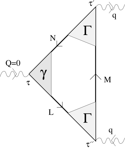
FIG. 1.: One of the two diagrams contributing to the triangle function given by Eq. (8). The Green functions (solid lines) are indexed by quantum numbers characterizing the Landau levels in the Landau gauge. The propagators are ‘dressed’ by interactions with impurities (as shown in Fig. 2(a)); consistent with the Ward identity charge vertex functions $\Gamma$ and current vertex functions $\gamma$ are included. Note this diagram excludes some negligible contributions (see Fig. 4(a), Ref. [25]). We assume short-range scatterers, which implies that $\gamma$ can be neglected and hence $L=N\pm 1$.

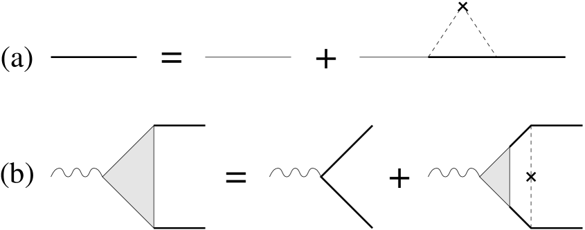
FIG. 2.: The impurity scattering is accounted for by the self-consistent Born approximation illustrated in (a). Thin lines are bare Green functions and thick lines are dressed Green functions. The dashed lines symbolizes interactions with impurities (crosses). Consistent with the self-consistent Born approximation, the charge vertex function should be taken as a ladder sum shown in (b).

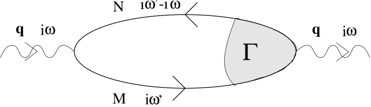
FIG. 3.: The density–density correlation function. Solid lines are dressed Green functions and the shaded area is the charge vertex function. The proper polarization function is obtained by doing analytical continuation, $i\omega\rightarrow\omega+i\eta$. The explicit expression is given in Eq. (52).

FIG. 4.: The two ingredients ‘effective interaction’ and ‘phase-space’ as a function of filling factor for fixed $(q,\omega)=(0.2/k_{F},0.001\varepsilon_{F}/\hbar)$ where $\varepsilon_{F}$ is the Fermi energy. The temperature is given by $T/T_{F}=0.01$. The dashed curve is the square of the effective interaction $|V_{21}(q)/{\mathcal{E}}(q,\omega)|^{2}$ in units of $g_{0}^{-2}=(\pi\hbar^{2}/m^{*})^{2}$, the dotted curve is ’the phase–space’ $[{\mathrm{I}m}\Pi(q,\omega)/\sinh(\hbar\omega/2k_{B}T)]^{2}$ in units of $(10g_{0})^{2}$. The solid line is (80 times) the product of the two.

FIG. 5.: The transresistivity as a function of filling factor for temperature $T=1.2$ K and interlayer distance $d=800$ Å. The density of the electron gases is $n_{1}=n_{2}=3\times 10^{15}\ {\rm m}^{2}$ and the mobility is 25 m²/Vs. Spin splitting has been neglected. The transresistivity shows a twin-peak structure: as the filling factor is changed from an odd value (where the highest Landau level is half filled) towards an even value, the transresistivity goes through a maximum before it gets suppressed. ($\rho_{21}$ has a maximum of 1.16 $\Omega$ at $\nu=1.8$ — out of the range of the plot).

FIG. 6.: The scaled transresistivity $\rho_{21}/T^{2}$ as a function of temperature for filling factors $\nu=3$ (solid line) and $\nu=5$ (dashed line). Other parameters are as in Fig. 5. $\rho_{21}/T^{2}$ which in zero magnetic field is expected to be a constant, shows a maximum as a function of $T$ in intermediate magnetic fields. The enhancement arises at a temperature which is related to the width of the Landau levels as explained in the main text.

FIG. 7.: The scaled transresistivity $\rho_{21}/T^{2}$ as a function of $T$ for three filling factors, $\nu=2.6$ (dotted line), $\nu=3.0$ (solid line), $\nu=3.3$ (dashed line). Other parameters are as in Fig. 5. The temperature $T_{\rm peak}$ at which $\rho_{21}/T^{2}$ has a maximum depends on $\nu$. $T_{\rm peak}$ as a function of $\nu$ is plotted in the inset. There is a maximum around $\nu=2.8$, i.e. just below an odd filling factor.

FIG. 8.: The function ${\mathcal{I}}(q,n,m)$ as a function of $m$ for $n=1$ (circles), and $n=3$ (triangles). In both cases $\ell q=0.35$.

REFERENCES

- [1] M. B. Pogrebinskii, Sov.Phys.Semicond., 11, 372 (1977);
- [2] P. J. Price, Physica, 117B, 750, (1983).
- [3] T. J. Gramila, J. P. Eisenstein, A. H. MacDonald, L. N. Pfeiffer, and K. W. West, Phys.Rev.Lett. 66, 1216 (1991); T. J. Gramila, J. P. Eisenstein, A. H. MacDonald, L. N. Pfeiffer, and K. W. West, Surf.Sci. 263, 446 (1992); T. J. Gramila, J. P. Eisenstein, A. H. MacDonald, L. N. Pfeiffer, and K. W. West, Phys.Rev.B. 47, 12957 (1993).
- [4] U. Sivan, P. M. Solomon, and H. Shtrikman, Phys.Rev.Lett. 68, 1196 (1992).
- [5] H. C. Tso, P. Vasilopoulos, and F. M. Peeters, Phys.Rev.Lett. 70, 2146 (1993); L. Swierkowski, J. Szymanski, and Z. W. Gortel, Phys.Rev.Lett. 74, 3245 (1995).
- [6] A.-P. Jauho, and H. Smith, Phys.Rev.B. 47, 4420, (1993).
- [7] L. Zheng, and A. H. MacDonald, Phys.Rev.B. 48, 8203 (1993); L. Zheng, Ph. D. thesis (Indiana Univ., 1993).
- [8] K. Flensberg, and B. Y.-K. Hu, Phys.Rev.Lett. 73, 3572 (1994)
- [9] K. Flensberg, and B. Y.-K. Hu, Phys.Rev.B. 52, 14796 (1995)
- [10] G. Vignale, and A. H. MacDonald, Phys.Rev.Lett. 76, 2786 (1996).
- [11] N. P. R. Hill, J. T. Nicholls, E. H. Linfield, M. Pepper, D. A. Ritchie, G. A. C. Jones, B. Y.-K. Hu, and K. Flensberg, Phys.Rev.Lett. 78, 2204 (1997).
- [12] H. C. Tso, P. Vasilopoulos, and F. M. Peeters, Phys.Rev.Lett. 68, 2516 (1992); C. Zhang, and Y. Takahashi, J.Phys.Cond.Matt 5, 5009 (1993); M. C. Bønsager, B. Y.-K. Hu, K. Flensberg, and A. H. MacDonald, to be published.
- [13] N. P. R. Hill, J. T. Nicholls, E. H. Linfield, M. Pepper, D. A. Ritchie, A. R. Hamilton, and G. A. C. Jones, J.Phys.: Cond.Matt 8, L557 (1996).
- [14] H. Rubel, A. Fischer, W. Dietsche, K. von Klitzing, and K. Eberl, Phys.Rev.Lett. 78, 1763 (1997).
- [15] X. Feng, H. Noh, S. Zelakiewicz, and T. J. Gramila, Bull. Am. Phys. Soc. 42, 487 (1997)
- [16] J. P. Eisenstein, L. N. Pfeiffer, and K. W. West, Bull. Am. Phys. Soc. 42, 486 (1997)
- [17] See e.g. Perspectives in Quantum Hall Effects, edited by S. Das Sarma and A. Pinczuk, (Wiley, New York, 1997).
- [18] S. M. Girvin, and A. H. MacDonald in Chapter 5 of Ref. [17].
- [19] M. C. Bønsager, K. Flensberg, B.Y.-K. Hu, and A.-P. Jauho, Phys.Rev.Lett. 77, 1366 (1996).
- [20] J. T. Chalker, and G. J. Daniell, Phys.Rev.Lett. 61, 593 (1988).
- [21] E. Shimshoni, and S. L. Sondhi, Phys.Rev.B. 49, 11484 (1994).
- [22] B. I. Halperin, P. A. Lee, and N. Read, Phys.Rev.B. 47, 7312 (1993). See also B. I. Halperin in Chapter 6 of Ref. [17].
- [23] Y. B. Kim, and A. J. Millis, cond-mat/9611125; S. Sakhi, cond-mat/9612028; I. Ussishkin, and A. Stern, cond-mat/9701135.
- [24] A. Kamenev, and Y. Oreg, Phys.Rev.B. 52, 7516 (1995).
- [25] K. Flensberg, B. Y.-K. Hu, A.-P. Jauho, and J. M. Kinaret, Phys.Rev.B. 52, 14761 (1995).
- [26] G. D. Mahan, Many-Particle Physics, 2nd Edition, Plenum Press, New York (1990).
- [27] T. Ando, and Y. Uemura, Journ.Phys.Soc.Japan 36, 959 (1974).
- [28] B. Y.-K. Hu, Phys. Scr. T69, 170 (1997).
- [29] Three independent experiments show this trend. We are grateful to Nick Hill, Holger Rubel, and Tom Gramila for discussing their unpublished experiments with us.
- [30] R. B. Gerhardts, Z. Phys. B 21, 275 (1975); ibid. 21 285 (1975).
- [31] See e.g. D. Forster, Hydrodynamic Fluctuations, Broken Symmetry, and Correlation Functions (Addison-Wesley, 1990).
- [32] M. W. Wu, H. L. Cui, and N. J. M. Horing, Mod. Phys. Lett. B. 10, 279 (1996).
- [33] The phonon contribution, as discussed in Ref. [12], also contributes a peak in at approximately the same temperatures at . Similar behavior may occur at finite . However, a detailed calculation is needed in order to determine the relative contributions of the Coulomb versus the phonon mediated interaction at .