Conductance and its universal fluctuations in the directed network model at the crossover to the quasi-one-dimensional regime

Abstract

The directed network model describing chiral edge states on the surface of a cylindrical 3D quantum Hall system is known to map to a one-dimensional quantum ferromagnetic spin chain. Using the spin wave expansion for this chain, we determine the universal functions for the crossovers between the 2D chiral metallic and 1D metallic regimes in the mean and variance of the conductance along the cylinder, to first nontrivial order.

]

I Introduction

Mesoscopic disordered conductors have attracted many theoretical and experimental investigations in recent years. The transport properties of chiral edge states on the boundary of a two-dimensional quantum Hall state have been of particular interest. Recently, attention [1, 2, 3, 4, 5, 6, 7] has focussed on a layered three-dimensional (3D) system consisting a large number of such quantum Hall systems stacked upon each other. Chalker and Dohmen [1] argued that the localized electronic states in the bulk of a quantum Hall system will remain localized even in the presence of a coupling in the third dimension, provided this coupling is not too strong. Electronic transport in such a system is therefore controlled by the itinerant, chiral, edge states, which now form a two-dimensional surface sheath on the boundary of the 3D sample. A recent experiment [8] on a GaAs/${\rm Al}_{0.1}{\rm Ga}_{0.9}$As multilayer structure has indeed found that the conductivity perpendicular to the layers scales with the perimeter of the sample when the bulk is in a layered quantum Hall state, thus demonstrating the existence of a conducting surface sheath.

Theoretical analyses of transport in this chiral surface sheath have so far been carried out in the context of a directed network model (DN) introduced by Chalker and Dohmen [1]. This model ignores electron-electron interactions and describes the motion of independent electrons along the links of a directed network; scattering events occur at the nodes of the network and we are ultimately interested in the probability distribution of transport coeffecients after the random scattering matrix element has been averaged over. The global phase diagram of the DN model is summarized in Fig 1.

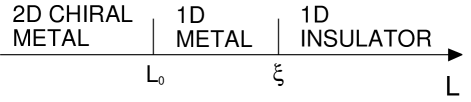
FIG. 1.: Sketch of the crossovers as a function of the length $L$. The first crossover [4] is at the scale $L_{0}=(C\rho_{s}/M_{0})^{1/2}$, where $\rho_{s}$ and $M_{0}$ are related to microscopic length and energy scales in a manner discussed below (2) and in Ref. [7]. The second crossover is near the localization length $\xi=8C\rho_{s}$. The conditions for the validity of the continuum theory require $\xi\gg L_{0}$, and so the two crossover scales are well separated. The 2D chiral metal regime was called 0D in Ref. [4], but we prefer the present terminology for reasons discussed in Ref. [7].

We are considering a surface sheath of length $L$ perpendicular to the layered quantum Hall states, and circumference $C$ along the chiral edges. The system therefore has the geometry of a cylinder of length $L$ and circumference $C$, and we discuss the results of two-terminal transport measurements with leads placed at the ends of the cylinder. As a function of $L$, there are three distinct coherent transport regimes, separated by the lengths $L_{0}$ and $\xi$ at which there are smooth crossovers. The precise values of these lengths will be discussed later, but here we simply note that $L_{0}\sim(Ca_{x})^{1/2}$ and $\xi\sim C$, where $a_{x}$ is a microscopic length of order the spacing between the layers. In the presence of electron-electron interactions there will also be a temperature-dependent phase coherence length $L_{\varphi}$ which arises from inelastic scattering events between electrons. This length must be accounted for in any comparison with experiments. In this paper we will, for simplicity, not consider electron-electron interactions and, therefore, our results can only be applied when the temperature is sufficiently low so that $L_{\varphi}\gg L,C$.

Let us now review the basic physical properties of the three regimes in Fig 1:
(i) 2D Chiral Metal: In the plane of the layers, the electrons move ballistically in a single direction along the surface (the chiral edge states), while transverse to the layers the motion is diffusive. As the transverse length $L<C^{1/2}$, the electrons do not have enough time to execute one chiral orbit in the plane before exiting through one of the ends of the system. The nomenclature “2D chiral metal” was suggested in Ref [7], from an interpretation of the structure of conductance fluctuations. Earlier work [4] has referred to this regime as 0D.
(ii) 1D Metal: The motion is as in the 2D chiral metal, but the system is now long enough that the electrons execute many chiral transverse orbits before leaving through one of the ends of the cylinder. The probability distribution of the transverse conductance is now very similar to that of a short metallic wire [7].
(iii) 1D Insulator: If the cylinder is long enough, eventually the one-dimensional diffusive motion along the axis of the cylinder undergoes Anderson localization [1], and the system behaves like an insulating wire [7].

We now outline the results obtained in earlier studies of the DN model. Ref [1] presented numerical studies which obtained the crossover to the 1D insulator. A mapping of the DN model to a ferromagnetic spin chain model was obtained in Ref [3]. Ref [4] studied the energy level fluctuations exclusively in the 2D chiral metal. In our previous work [7] (hereafter referred to as I), we obtained explicit results for the crossovers in the conductance and its variance between the 1D metal and the 1D insulator regimes: these results were in good agreement with the earlier numerical work [1]. Refs [5] and [6] presented an incomplete description of the conductance fluctuations in the 2D chiral metal regime, and argued these were non-universal.

The present paper contains a detailed and complete description of the crossover between the 2D chiral metal and 1D metal, along with explicit and exact expressions for universal crossover functions describing the behavior of the conductance and its variance. In contrast to earlier work [5, 6] we find that the variance of the conductance, and all of its higher moments, are universal when suitably expressed in terms of a small number of renormalized parameters which characterize the microscopic theory: the relationship between our and earlier [5, 6] results will be discussed in greater detail in the body of the paper.

II Definition of the model and outline of results

The formalism and results of this paper are a continuation of those presented in I. We will therefore not repeat here the detailed discussion of the structure of the DN model presented in I. It was shown in I (and in Refs [3, 4]) that the DN model can be mapped onto a continuum quantum field theory for a 1D quantum ferromagnet in “imaginary time”. Here the co-ordinate along the circumference of the cylinder (of length $C$) is interpreted as the “imaginary time” direction of a one-dimensional quantum system whose degrees of freedom reside along the “space” direction of length $L$. The mapping involves an average over disorder, which is performed using either replica or supersymmetry methods. In the first case the quantum ferromagnet contains spins of the su($n$,$n$) or su($2n$) algebra, depending on whether we use bosonic or fermionic replicas, and we are interested in the limit $n\to 0$. In the second case the spins are generators of a superalgebra. In the present paper, we will be interested in the perturbative spin-wave expansion, and for this purpose it is more convenient to use a bosonic replica formalism rather than supersymmetry. Although replicas are known to fail in some non-perturbative situations [9] (but not in all, see for example Ref. [10]), for perturbative calculations they are completely equivalent to the supersymmetry method. If one uses, then, the bosonic replica formalism to treat the disorder averages, the ferromagnet action is (the reader is urged to consult our companion paper I for further details)

$$S_{\rm cont} = -\int_{0}^{L}\!\!\!dx\!\int_{0}^{C}\!\!\!d\tau\left({M_{0}\over 2}\int_{0}^{1}\!\!\!du\,{\rm tr}Q(u)\partial_{u}\!Q(u)\partial_{\tau}\!Q(u)\right.$$ (2)

$$\left.\vphantom{\int_{0}^{1}\!\!\!du}+{\rho_{s}\over 2}{\rm tr}(\partial_{x}Q)^{2}\right),$$

where $M_{0}$ and $\rho_{s}$ are the magnetization per unit length, and the spin stiffness in the ground state respectively. $Q(x,\tau)$ is a $2n\times 2n$ matrix obeying $Q^{\dagger}=\Lambda Q\Lambda$, where $\Lambda$ is a diagonal matrix with elements $(1,\ldots,1,-1,\ldots,-1)$, $Q^{2}=I$, and having $n$ eigenvalues 1, $n$ eigenvalues $-1$, which thus parametrizes the coset space SU($n$,$n$)/S(U($n$)$\times$U($n$)). In the Berry phase term, the first term in (2), $Q(u)\equiv Q(x,\tau,u)$ is some smooth homotopy between $Q(x,\tau,0)=\Lambda$ and $Q(x,\tau,1)=Q(x,\tau)$. The field $Q$ satisfies the periodic boundary condition in the $\tau$-direction, and the following boundary conditions at the spatial boundary, where the DN is connected to ideal leads:

$$Q(0,\tau,u)=Q(L,\tau,u)=\Lambda.$$ (3)

This paper shall focus exclusively on the properties of $S_{\rm cont}$, which the reader can also consider as a ferromagnet of super/replica spins of interest in its own right. It was argued in I that the properties of the DN model are completely, and universally, characterized by the dimensionful parameters that appear in $S_{\rm cont}$: these are $\rho_{s}$, $M_{0}$, $L$ and $C$. Of these, $L$ and $C$ are given by the macroscopic dimensions of the sample, and therefore easily measured. The values of $\rho_{s}$ and $M_{0}$ are determined by the detailed microscopic properties of the electronic system; nevertheless if the microscopic Hamiltonian is precisely known, the exact values of $\rho_{s}$ and $M_{0}$ can usually be determined exactly [7]. This is in contrast to the conventional case in the theory of critical phenomena, where the relationship of renormalized parameters to the underlying microscopics requires solution of an intractable, strongly-coupled problem.

We comment briefly on aspects of the relationship between the values of $\rho_{s}$ and $M_{0}$ for the DN model as introduced in Ref. [1], and studied in I. For the case in which the interior of the cylinder is supposed to be a quantized Hall state with Hall conductance per layer equal to 1 (in units of $e^{2}/h$), the parameter $M_{0}$ takes the value [7] $1/2a_{x}$, where $a_{x}$ is the separation of the layers, while $\rho_{s}$ involves also other parameters that need not be specified here [7]. Here we wish to argue that, for the more general situation in which the bulk Hall conductance is an integer $\nu>0$, say, and there are $\nu$ chiral edge channels on the edge of each layer, the appropriate model for the large scale properties is again the model with action Eqn. (2), but with $M_{0}=\nu/2a_{x}$, where $a_{x}$ is still the separation of the layers. This ensures that the edge channels have the correct total conductance for transport along the edges, but the details of the distinct channels are unimportant, assuming that there is hopping of similar strength between all nearby channels. If the hopping between the different edge channels in a layer is much weaker than that between corresponding channels in different layers, then the theoretical mappings of Refs. [3, 4] and I lead to $\nu$ ferromagnetic superspin chains with weak ferromagnetic coupling between them. Such couplings are relevant and cause the behavior to cross over on large length scales to that for a single chain with $M_{0}=\nu/2a_{x}$. (The relation among the values of $\rho_{s}$ for these different regimes is a little more complex; it can be calculated by considering the excited states of the coupled chains with a single spin flipped, in the long wavelength limit.) It is possible that in practise a given sample with $\nu>1$ might not be large enough to reach this regime, and the comparison of experimental data with the following theory might then be complicated by crossover effects. These crossover effects will not be further addressed here, but could be studied by similar methods to those below.

There are three distinct regimes in the theory described by $S_{\rm cont}$, identified by Balents et al. in Ref. [4], which were shown earlier in Fig 1. We can now quote the precise values of the scales $L_{0}$, $\xi$, at which the crossovers take place:

$$L_{0}=(C\rho_{s}/M_{0})^{1/2}$$ (4)

and

$$\xi=8C\rho_{s}.$$ (5)

The physics of both 1D regimes was discussed in detail in I, where it was shown that for $L\gg L_{0}$, the action for the quantum continuum ferromagnet may be further reduced to that of a 1D non-linear sigma model. This latter model has been extensively studied in the context of quasi-1D wires, see, in particular, Ref. [11]; using these earlier results, explicit formulas for the mean and variance of the conductance of $S_{\rm cont}$ were given in I, valid thoughout the crossover between the 1D metallic and 1D localized regimes.

In this paper we concentrate on the conduction properties in the 2D chiral metal regime $L\ll L_{0}$ and the crossover to the 1D metallic regime $L_{0}\ll L\ll\xi$. The model with action $S_{\rm cont}$ represents a continuum su($n$,$n$) ferromagnet at finite effective temperature $1/C$ (this effective temperature, which is really the inverse circumference, $1/C$, plays a very different role than the true temperature, which is essentially zero, would). It was argued in Ref [4] and I, that when the effective temperature $1/C$ becomes less than the order of the low-lying level splittings of spin waves or magnons, which are of order $\rho_{s}/M_{0}L^{2}$, there are very few thermally excited magnons, and the problem can be treated perturbatively. This defines the 2D chiral metal regime, $1/C\ll\rho_{s}/M_{0}L^{2}$, or $L\ll L_{0}$. In the 1D metallic regime, the temperature $1/C$ is larger than the splittings, but the thermally excited magnons can be viewed as a slow variation of the spin direction with position and imaginary time. In this regime, the classical statistical mechanics approximation of neglecting the time dependence can be used, and leads to the 1D non-linear sigma model, with coupling constant $\sim 1/C\rho_{s}$. Perturbation theory breaks down on long length scales, but is still valid when the length $L$ is less than the localization length $\xi=8C\rho_{s}$. Thus, spin-wave perturbation theory can be used all the way across the 2D to 1D crossover. In particular, the scaling forms of the mean and variance of the conductance can be expanded as a perturbation series in powers of $L/\xi$, times a universal function of $L/L_{0}$ in each term. In this paper we will show explicitly that for $\langle g\rangle$, the mean of $g$ (here and below, the single angular brackets $\langle\ldots\rangle$ denote the average of a quantity over the disorder), this takes the form (here and henceforth, all conductances are quoted in units of $e^{2}/h$):

$$\langle g\rangle=\xi/2L+(L/\xi)\Phi\left(L/L_{0}\right)+O\left((L/\xi)^{2}\right).$$ (6)

To leading order in $L/\xi$ there is no dependence on $L/L_{0}$ (Ref. [1]). We will show below that the possible term of order $(L/\xi)^{0}$ vanishes identically, consistent with the known result that the leading “weak localization” correction to $\langle g\rangle$ vanishes in the quasi-1D metallic regime $L/L_{0}\to\infty$ in the present (unitary) case. The next term in the expansion in $L/\xi$ in (6) does have a non-trivial crossover at the scale $L_{0}$, described by a universal function $\Phi$ given below in Eq. (10). In contrast, for the variance of $g$ we obtain

$${\rm var}\,g\equiv\langle g^{2}\rangle-{\langle g\rangle}^{2}=\widetilde{\Phi}\left(L/L_{0}\right)+O\left(L/\xi\right),$$ (7)

where the universal crossover from the 2D to the 1D metallic regime is evident in the leading term $\widetilde{\Phi}$ given below in Eq. (11). This leading term, which is all that survives in the limit $L/\xi\rightarrow 0$, corresponds to what are known as “universal conductance fluctuations” (UCF), which are similarly the weak coupling limit of the crossover function. Note that we use the term “universal” as it is understood in critical phenomena, to mean that the results are independent of microscopic details of the model, and that the conductance fluctuations are described by a universal function of the sample geometry (that is, in the present case, of $L/L_{0}$). This should be contrasted with the usage often implicit in the mesoscopic physics literature, in which “universal” stands for the value $e^{2}/h$. In such usage, anything close to this value is called universal. For us, on the other hand, this unit of conductance is left implicit in our formulas, and it is the numerical coefficient, which is actually a precise function of $L/L_{0}$, that is universal in our sense, and need not even be close to unity, as in the results below. These considerations apply unchanged to the conventional UCF, which in our opinion are best regarded in this sense also.

The universal functions $\Phi$ and $\widetilde{\Phi}$ are calculated in the following sections, and the results are

$$\Phi\left(L/L_{0}\right) = {4\lambda^{2}\over\pi^{4}}\left(\left(\sum_{l=1}^{\infty}f(\lambda l^{2})\right)^{2}+{1\over 2}\sum_{l=1}^{\infty}f^{2}(\lambda l^{2})\right.$$ (10)

$$\mbox{}+\!\!\sum_{l_{1},l_{2},l_{3}=1}^{\infty}{l_{3}^{2}\over l_{1}^{2}+l_{2}^{2}-l_{3}^{2}}{f(\lambda l_{1}^{2})f(\lambda l_{2}^{2})f(-\lambda l_{3}^{2})\over f\left(\lambda(l_{1}^{2}+l_{2}^{2}-l_{3}^{2})\right)}$$

$$\left.\vphantom{\left(\sum_{l=1}^{\infty}\right)^{2}}\times\left(\delta_{l_{1},l_{2}+l_{3}}+\delta_{l_{2},l_{1}+l_{3}}+\delta_{l_{3},l_{1}+l_{2}}\right)\right),$$

$$\widetilde{\Phi}\left(L/L_{0}\right) = {\lambda\over 3\pi^{2}}+{2\lambda\over\pi^{4}}\sum_{l=1}^{\infty}f(\lambda l^{2})\!\left(2/l^{2}-\lambda f(-\lambda l^{2})\right).$$ (11)

In these expressions $\lambda=2\pi^{2}L_{0}^{2}/L^{2}$, and $f(x)=1/(e^{x}-1)$ is the Bose function. These expressions are easily evaluated numerically, and the resulting plots are shown in Fig. 2.

Using the limiting behaviour of $f(x)$ for small and large values of $x$ we obtain from Eqs. (10,11) in the 1D limit $L/L_{0}\rightarrow\infty$ (but still with $L/\xi\ll 1$) of long cylinders

$$\Phi\left(L/L_{0}\right) \to -{2\over 45},$$ (12)

$$\widetilde{\Phi}\left(L/L_{0}\right) \to {1\over 15}.$$ (13)

These limits (12,13) for long cylinders are the well known quasi-1D metallic results [11]. In the opposite 2D chiral limit $L/L_{0}\rightarrow 0$ of short cylinders

$$\Phi\left(L/L_{0}\right) \sim -{16L_{0}^{4}\over L^{4}}\exp\left(-{2\pi^{2}L_{0}^{2}\over L^{2}}\right),$$ (14)

$$\widetilde{\Phi}\left(L/L_{0}\right) \sim {2L_{0}^{2}\over 3L^{2}}.$$ (15)

FIG. 2.: Plots of the universal functions $\Phi$, for the correction to the mean conductance (top), and $\widetilde{\Phi}$, for the variance of the conductance (bottom). The dashed and dot-dashed lines are plots of the asymptotic expressions at small and large values of $L/L_{0}$, Eqs. (14,15) and (12,13), respectively.

As an alternative to the interpretation above in terms of thermally excited magnons, we can also understand the results for this crossover in terms of the sum over paths taken by the propagating electrons. To calculate the conductance, retarded and advanced paths are required, and these are paired up by the average over the disorder. This was the basis for the treatment in I. For $\langle g\rangle$, the leading term comes from paired paths that go from one end to the other of the system while propagating a distance of order $M_{0}L^{2}/\rho_{s}$ around the circumference. This distance is $\ll C$ in the 2D regime. Therefore the corrections (which correspond to thermally-excited magnons) in the series in $L/\xi$ for $\langle g\rangle$, which reflect the effect of paired paths that wind around the finite circumference and interfere with themselves, are exponentially small in this limit. In contrast, for ${\rm var}\,g$, there are nontrivial effects at leading (zeroth) order in $L/\xi$, which, like the leading term in $\langle g\rangle$, do not require winding paths. The correction terms to the behavior in Eq. (15) are also exponentially small in the 2D chiral metal regime. Note that nontrivial effects in the absence of winding paths also appeared in Refs. [11, 5].

A result of the form of Eq. (15) for ${\rm var}\,g$, has been claimed by Mathur [5] and Yu [6], who find ${\rm var}\,g\propto C\rho_{s}/M_{0}L^{2}$ in the limit $L\ll L_{0}$. Mathur’s explanation of this result, which is essentially that the sample can be divided into blocks of size of order $L\times M_{0}L^{2}/\rho_{s}$ which have statistically-independent fluctuations with variance of order $1$ that add to give ${\rm var}\,g$, appears correct. However, both he and Yu [6] state that this result is nonuniversal, and Yu bases this statement on its dependence on $\rho_{s}/M_{0}$ (in our notation). Mathur’s results are incomplete, as stated by him. His result for $L\ll L_{0}$ (but not that for $L\gg L_{0}$) does agree with ours in this limit for fortuitous reasons which will be discussed in Sec. V. Yu [6] states that his results are nonperturbative, but fail for some parameter values. In contrast, we are able not only to compute the mean and variance of the conductance in the limiting cases, but also to determine the full crossover functions. We have already commented above on the meaning of universality and the scaling with $L/L_{0}$, and we argue that the crossover functions are universal in the domain of applicability of the continuum description of the DN model. Our calculation shows that this crossover from 2D to 1D metal can be treated perturbatively in close analogy to the usual UCF in an isotropic diffusive system, where one can also treat the crossover from 2D to 1D. (Here we would like to repeat a remark already made in I, that in the latter case, for a sample of width $W$ and length $L$, one finds ${\rm var}\,g\propto W/L$ as $W/L\rightarrow\infty$. This behavior can be understood by viewing the sample as composed of independent blocks of size $L\times L$. It is nonetheless universal in the sense we prefer, as discussed above. It is true that here there is no dependence on the conductivity, while there is in the chiral metal, but this does not mean the result for the latter is nonuniversal, because the scaling functions for the chiral metal exhibit no-scale-factor universality, as argued in I, so the dependence on the bare coupling constants $\rho_{s}$ and $M_{0}$ is meaningful.) In addition, our results differ quantitatively from those of Yu [6]. Thus our results differ from those in either of Refs. [5, 6].

The rest of the paper presents the details in the computation of the central results (10) and (11). Beginning in the next section, we develop the spin wave expansion mentioned above. The su($n$,$n$) spin chain is described in Sec. III. In the same section we introduce a parametrization for the spins in terms of Dyson-Maleev (DM) bosons. In Sec. IV we exploit gauge invariance to obtain expressions for the currents and for the moments of the conductance in terms of DM bosons. Details of the perturbative calculations are given in Sec. V. Finally, we conclude in Sec. VI.

III Spin wave expansion in terms of Dyson-Maleev bosons

In this section we will begin by considering a lattice discretization of $S_{\rm cont}$ and then set up a spin-wave perturbation theory using the Dyson-Maleev method.

In I we used supersymmetry to treat the disorder averages in the mapping of the DN to a spin chain. When the mapping is performed instead (in a completely parallel way) using bosonic replicas we obtain the following Hamiltonian for the spin chain:

$${\cal H}=K\sum_{i=1}^{N-1}{\rm tr}\left(J(i)J(i\!+\!1)+{1\over 2}\Lambda\left(J(1)+J(N)\right)\right).$$ (16)

Here the $J$ are the su($n$,$n$) spins in a particular irreducible representation. This representation naturally appears in the mapping as follows. We introduce $n$ “retarded” and $n$ “advanced” bosons $a_{i},b_{i}$, $i=1,2,\ldots,n$. Their bilinear products obeying u($n$,$n$) commutation relations are arranged in a $2n\times 2n$ matrix

$$J = \left(\begin{array}[]{cc}{1\over 2}\delta_{ik}+a^{\dagger}_{i}a_{k}&a^{\dagger}_{i}b^{\dagger}_{l}\\ -b^{\vphantom{\dagger}}_{j}a^{\vphantom{\dagger}}_{k}&{1\over 2}\delta_{jl}-b^{\vphantom{\dagger}}_{j}b^{\dagger}_{l}\end{array}\right)$$ (19)

The average over randomness in the DN model produces the local constraint $a^{\dagger}_{i}a^{\vphantom{\dagger}}_{i}=b^{\dagger}_{i}b^{\vphantom{\dagger}}_{i}$ (we assume summation over repeated indices everywhere, unless stated otherwise). The subspace of the Fock space of bosons specified by this constraint forms a highest weight irreducible representation of the algebra su($n$,$n$) with the vacuum $|0\rangle$ being the highest weight state.

The trace in Eq. (16) is over the matrix indices of the spins which are multiplied as matrices. The last term in Eq. (16) comes from the boundary, where the DN is connected to the ideal leads. $\Lambda$ is the same as in (3).

The mean conductance $\langle g\rangle$ is given by the thermal correlator of conserved currents

$$\langle g\rangle=-{\rm Tr}\left({\cal T}I(i)I(j)e^{-C{\cal H}}\right),$$ (20)

for $i\neq j$, where $\rm Tr$ stands for the quantum mechanical trace in the Hilbert space, the role of the inverse temperature is played by the circumference $C$ of the cylinder, the currents $I(i)$ are related to the spins (see I), and $\cal T$ is the time-ordering operator. Similar expressions can be given for the moments of the conductance.

For the perturbative spin wave expansion it is convenient to make use of another construction of the necessary representation of su($n$,$n$). It is very similar to the Dyson-Maleev construction [13] of representations of su($2$) and proceeds as follows. We introduce $n^{2}$ bosons, which we arrange in an $n\times n$ matrix ${\hat{b}}$ with elements ${\hat{b}}_{ij}$, $i,j=1,\ldots,n$. To avoid confusion, we will denote boson creation operators by an asterisk: ${\hat{b}}^{*}_{ij}$, and reserve the dagger for the hermitean conjugate of matrices of operators. Then the hermitean conjugate matrix ${\hat{b}}^{\dagger}$ has elements $({\hat{b}}^{\dagger})_{ij}={\hat{b}}^{*}_{ji}$. We also assume that whenever we write a product of several ${\hat{b}}$’s and ${\hat{b}}^{\dagger}$’s without indices, it means the usual matrix product. These $n^{2}$ bosons satisfy canonical commutation relations $[{\hat{b}}^{\phantom{*}}_{ij},{\hat{b}}^{*}_{kl}]=\delta_{ik}\delta_{jl}$. Then the su($n$,$n$) spin $J$ is given in block-matrix form by

$$J=\left(\begin{array}[]{cc}{1\over 2}+{\hat{b}}^{\dagger}{\hat{b}}&{\hat{b}}^{\dagger}\\ (n-1-{\hat{b}}{\hat{b}}^{\dagger})b&n-{1\over 2}-{\hat{b}}{\hat{b}}^{\dagger}\end{array}\right).$$ (21)

When we substitute this expression for the spins $J$ in terms of DM bosons into the Hamiltonian (16) and bring them to normal order, we obtain, in particular, quartic terms which do not have the matrix product index structure. Next we introduce a bosonic functional integral using bosonic coherent states $|b\rangle$ satisfying ${\hat{b}}|b\rangle=b|b\rangle$. In this functional integral the bosonic operators ${\hat{b}}$ are replaced by commuting variables $b$ (without a hat), and we can bring the quartic terms back to the usual matrix product form. This gives the following action:

$$S = \int_{0}^{C}\!\!\!d\tau\sum_{i}{\rm tr}\left(b^{\dagger}(i)\partial_{\tau}\!b(i)\right.$$ (24)

$$\mbox{}+K\left(b^{\dagger}(i\!+\!1)-b^{\dagger}(i)\right)\left(b(i\!+\!1)-b(i)\right)$$

$$\left.-Kb^{\dagger}(i)\left(b(i\!+\!1)-b(i)\right)b^{\dagger}(i\!+\!1)\left(b(i\!+\!1)-b(i)\right)\!\right)$$

(we dropped a constant $n/2$ which disappears in the replica limit). The measure for the functional integral over $b$, $b^{\dagger}$ is the usual one, $D[b,b^{\dagger}]$.

Next we take continuum limit in the spatial direction and obtain the action $S=S_{0}+S_{\rm int}$, where

$$S_{0} = \int_{0}^{L}\!\!\!dx\!\int_{0}^{C}\!\!\!d\tau\,{\rm tr}\left(2M_{0}b^{\dagger}\partial_{\tau}\!b+4\rho_{s}\partial_{x}b^{\dagger}\partial_{x}b\right),$$ (25)

$$S_{\rm int} = -4\rho_{s}\int_{0}^{L}\!\!\!dx\!\int_{0}^{C}\!\!\!d\tau\,{\rm tr}\left(b^{\dagger}\partial_{x}bb^{\dagger}\partial_{x}b\right),$$ (26)

with $M_{0}=1/2a_{x}$ and $\rho_{s}=Ka_{x}$. The $\tau$-derivative term in $S_{0}$ does not have the canonical form. This could be mended by a rescaling of the bosonic fields. However, we will keep the present normalization to avoid cumbersome coefficients in different expressions appearing later. The boundary terms in the Hamiltonian (16) in the continuum description force the field $b(x)$ to take zero values at the boundaries:

$$b(0,\tau)=b(L,\tau)=0.$$ (27)

Before giving the expressions for the currents in terms of DM bosons and evaluating their correlators in the theory with the action (25,26), we note that the latter could have been obtained from $S_{\rm cont}$ of Eq. (2) by the following formal change of variables in the functional integral over the field $Q$:

$$Q=\left(\begin{array}[]{cc}1+2bb^{\dagger}&2b^{\dagger}\\ -2(1+bb^{\dagger})b&-1-2bb^{\dagger}\end{array}\right).$$ (28)

Even though this expression does not satisfy the original conditions on $Q$ (stated after Eq. 1), it formally coincides with $2\langle b|J|b\rangle$ where $J$ is given by (21) ($n$ in the lower left corner of (21) disappears after normal ordering the term ${\hat{b}}{\hat{b}}^{\dagger}$). Also, the SU($n$,$n$)-invariant functional measure for $Q$ reduces to $D[b,b^{\dagger}]$. These observations give us a very general and straightforward way of obtaining the expressions for the currents and the moments of the conductance. Namely, we have to make the action (2) gauge invariant by coupling to a gauge field. Then functional derivatives with respect to this field will give the currents and the moments of the conductance. When used together with Eq. (28), this procedure gives all the quantities in terms of DM bosons. In the next section we describe this procedure in detail.

IV Gauge invariance, current conservation and moments of conductance

It is clear from the last section that the distribution of the conductance of the DN model is related to correlators of the conserved current of the ferromagnetic spin chain. The computation of the required correlators is greatly simplified by an understanding of the gauge-invariance properties of $S_{\rm cont}$ which will be discussed in this section.

We can make the action (2) invariant under the local gauge transformation $Q\to{\tilde{Q}}=UQU^{-1}$, $A_{\mu}\to{\tilde{A}_{\mu}}=UA_{\mu}U^{-1}-iU\partial_{\mu}\!U^{-1}$, with $U\in$ SU($n$,$n$), by replacing the partial derivatives with the covariant ones: $\partial_{\mu}\!X\to D_{\mu}X\equiv\partial_{\mu}\!X+i[A_{\mu},X]$, where the gauge potential $A_{\mu}$ is an element of su($n$,$n$). However, as discussed in detail in Ref. [14], this is only necessary for the $(\partial_{x}Q)^{2}$ term. The Berry phase term, being a total derivative, can be made gauge invariant by adding a boundary term, and the gauge invariant action is

$$S[{\bf A}] = -\int_{0}^{L}\!\!\!dx\!\int_{0}^{C}\!\!\!d\tau\left({M_{0}\over 2}\int_{0}^{1}\!\!\!du\,{\rm tr}Q(u)\partial_{u}\!Q(u)\partial_{\tau}\!Q(u)\right.$$ (30)

$$\left.\vphantom{\int_{0}^{1}\!\!\!du}+i\,M_{0}{\rm tr}A_{\tau}Q+{\rho_{s}\over 2}{\rm tr}(D_{x}Q)^{2}\right).$$

Gauge invariance of this action implies some conservation laws, or Ward identities (WI’s). In their derivation we closely follow Ref. [14]. Let us introduce the generating functional

$$Z[{\bf A}]=\int\!\!D[Q]\,\exp\left(-S[{\bf A}]\right).$$ (31)

Using the notation

$$\left\langle\!\left\langle X\right\rangle\!\right\rangle=Z^{-1}[{\bf A}]\int\!\!D[Q]\,X[Q]\exp\left(-S[{\bf A}]\right),$$ (32)

where $X[Q]$ represents any functional of $Q$, we can show that gauge invariance of the action (30) results in the following equation of motion:

$$\left\langle\!\left\langle\delta S/\delta Q\right\rangle\!\right\rangle=0.$$ (33)

As shown in Ref. [14], this is equivalent to the following covariant current conservation law:

$$D_{\tau}\left\langle\!\left\langle j_{\tau}\right\rangle\!\right\rangle+D_{x}\left\langle\!\left\langle j_{x}\right\rangle\!\right\rangle=0,$$ (34)

where we introduced matrix-valued gauge invariant currents $j_{\mu}$ with elements

$$j_{\mu,ij}(x,\tau)\equiv-{\delta S[{\bf A}]\over\delta A_{\mu,ji}(x,\tau)}.$$ (35)

Equation (34) is the first in the series of WI’s coming from the gauge invariance. The gauge invariant currents $j_{\mu}$ (35) contain gauge potentials, and further WI’s are obtained differentiating with respect to ${\bf A}$. In particular, we can obtain such identities for the mean two-probe conductance and its variance, which in this field-theoretic formalism are obtained as follows. Let us assume that the source field ${\bf A}$ is independent of $\tau$, and moreover, has the special form

$$A_{\tau}=0,\quad A_{x}(x)=\left(\begin{array}[]{cc}A^{(1)}(x)&A^{+}(x)\\ A^{-}(x)&A^{(2)}(x)\end{array}\right).$$ (36)

Then the mean conductance is given by

$$\langle g(x,x^{\prime})\rangle=\lim_{{\scriptstyle n\to 0}\atop{\scriptstyle{\bf A}\to 0}}{\delta^{2}Z[{\bf A}]\over\delta A^{+}_{11}(x)\delta A^{-}_{11}(x^{\prime})}.$$ (37)

If we introduce the spatial currents integrated over $\tau$,

$$I_{ij}(x)=-{\delta S[{\bf A}]\over\delta A_{ji}(x)}=\int_{0}^{C}\!\!\!d\tau j_{x,ij}(x,\tau),$$ (38)

then

$$\langle g(x,x^{\prime})\rangle=\lim_{{\scriptstyle n\to 0}\atop{\scriptstyle{\bf A}\to 0}}{\delta\left\langle\!\left\langle I^{+}_{11}(x^{\prime})\right\rangle\!\right\rangle\over\delta A^{+}_{11}(x)}.$$ (39)

This differs from the formula for $\langle g\rangle$ earlier by including a contact term, and which was avoided then by the condition on the sites $i\neq j$.

With the choice (36) the WI (34) becomes

$$D_{x}\left\langle\!\left\langle I(x)\right\rangle\!\right\rangle=\partial_{x}\left\langle\!\left\langle I(x)\right\rangle\!\right\rangle+i[A_{x},\left\langle\!\left\langle I(x)\right\rangle\!\right\rangle]=0.$$ (40)

The current $I(x)$ has the same structure as $A(x)$:

$$I(x)=\left(\begin{array}[]{cc}I^{(1)}(x)&I^{+}(x)\\ I^{-}(x)&I^{(2)}(x)\end{array}\right),$$ (41)

and the $+$ component of (40) is simply

$$\partial_{x}\left\langle\!\left\langle I^{+}\right\rangle\!\right\rangle\!+\!i\left\langle\!\!\left\langle A^{+}I^{(2)}\!-\!I^{(1)}A^{+}\!+\!A^{(1)}I^{+}\!-\!I^{+}A^{(2)}\right\rangle\!\!\right\rangle=0.$$

Differentiating with respect to $A^{+}_{11}(x^{\prime})$ and using (39), we obtain

$$\partial_{x}\langle g(x^{\prime},x)\rangle+i\delta(x-x^{\prime})\lim_{{\scriptstyle n\to 0}\atop{\scriptstyle{\bf A}\to 0}}\left\langle\!\!\left\langle I^{(2)}_{11}(x)-I^{(1)}_{11}(x)\right\rangle\!\!\right\rangle=0.$$

In the next section we will show that the second term here vanishes in all orders of perturbation theory. As a consequence, the mean conductance is independent of the positions of cross section $x$. Similarly, it is independent of $x^{\prime}$ as well:

$$\partial_{x}\langle g(x,x^{\prime})\rangle=\partial_{x^{\prime}}\langle g(x,x^{\prime})\rangle=0.$$ (42)

This can be used to average $\langle g\rangle$ over these positions:

$$\langle g\rangle = {1\over L^{2}}\int_{0}^{L}\!\!\!dx\int_{0}^{L}\!\!\!dx^{\prime}\langle g(x,x^{\prime})\rangle$$ (43)

$$= {1\over L^{2}}\lim_{{\scriptstyle n\to 0}\atop{\scriptstyle{\bf A}\to 0}}\int_{0}^{L}\!\!\!dx\int_{0}^{L}\!\!\!dx^{\prime}\left\langle\!\!\!\left\langle{\delta I^{+}_{11}(x^{\prime})\over\delta A^{+}_{11}(x)}+I^{-}_{11}(x)I^{+}_{11}(x^{\prime})\right\rangle\!\!\!\right\rangle.$$ (44)

Similarly, the second moment is obtained by taking four derivatives:

$$\langle g(x_{1},x^{\prime}_{1})g(x_{2},x^{\prime}_{2})\rangle=$$ (45)

$$\lim_{{\scriptstyle n\to 0}\atop{\scriptstyle{\bf A}\to 0}}{\delta^{4}Z[{\bf A}]\over\delta A^{+}_{11}(x_{1})\delta A^{-}_{11}(x^{\prime}_{1})\delta A^{+}_{22}(x_{2})\delta A^{-}_{22}(x^{\prime}_{2})}.$$ (46)

Again we can show that this expression does not depend on any $x_{i}$, and we write

$${\rm var\,}g = {1\over L^{4}}\lim_{{\scriptstyle n\to 0}\atop{\scriptstyle{\bf A}\to 0}}\int_{0}^{L}\!\!\!dx_{1}\!\!\int_{0}^{L}\!\!\!dx^{\prime}_{1}\!\!\int_{0}^{L}\!\!\!dx_{2}\!\!\int_{0}^{L}\!\!\!dx^{\prime}_{2}$$ (53)

$$\left\langle\!\!\!\left\langle{\delta I^{+}_{11}(x^{\prime}_{1})\over\delta A^{+}_{11}(x_{1})}{\delta I^{+}_{22}(x^{\prime}_{2})\over\delta A^{+}_{22}(x_{2})}+{\delta I^{+}_{22}(x^{\prime}_{2})\over\delta A^{+}_{11}(x_{1})}{\delta I^{-}_{22}(x_{2})\over\delta A^{-}_{11}(x^{\prime}_{1})}\right.\right.$$

$$+{\delta I^{-}_{22}(x_{2})\over\delta A^{+}_{11}(x_{1})}{\delta I^{+}_{22}(x^{\prime}_{2})\over\delta A^{-}_{11}(x^{\prime}_{1})}$$

$$+{\delta I^{+}_{11}(x^{\prime}_{1})\over\delta A^{+}_{11}(x_{1})}I^{-}_{22}(x_{2})I^{+}_{22}(x^{\prime}_{2})+(1\leftrightarrow 2)$$

$$+{\delta I^{+}_{22}(x^{\prime}_{2})\over\delta A^{+}_{11}(x_{1})}I^{-}_{22}(x_{2})I^{+}_{11}(x^{\prime}_{1})+(1\leftrightarrow 2)$$

$$+{\delta I^{-}_{22}(x_{2})\over\delta A^{+}_{11}(x_{1})}I^{+}_{11}(x^{\prime}_{1})I^{+}_{22}(x^{\prime}_{2})+(+\leftrightarrow-)$$

$$+\left.\left.\vphantom{\delta I^{+}_{11}(x^{\prime}_{1})\over\delta A^{+}_{11}(x_{1})}I^{-}_{11}(x_{1})I^{+}_{11}(x^{\prime}_{1})I^{-}_{22}(x_{2})I^{+}_{22}(x^{\prime}_{2})\right\rangle\!\!\!\right\rangle_{\rm conn},$$

where the subtraction of $\langle g\rangle^{2}$ leaves only connected terms in the above expression.

Now we specify the gauge potential even further, leaving only the $A^{\pm}$ components nonzero, which is all we need to calculate moments of conductance. With this gauge choice we make the substitution (28) in the gauge invariant action $S[{\bf A}]$. The result is $S[{\bf A}]=S_{0}+S_{\rm int}+S^{\prime}[A_{x}]$, where $S_{0}$ and $S_{\rm int}$ are the same as before, Eqs. (25,26), and

$$S^{\prime}[A_{x}] = -4\rho_{s}\int_{0}^{L}\!\!\!dx\!\int_{0}^{C}\!\!\!d\tau\,{\rm tr}\left(iA^{-}(\partial_{x}b^{\dagger}-2b^{\dagger}\partial_{x}bb^{\dagger})\right.$$ (58)

$$\mbox{}+iA^{+}\left(\partial_{x}(b+bb^{\dagger}b)-2b\partial_{x}b^{\dagger}b+2bb^{\dagger}\partial_{x}bb^{\dagger}b\right)$$

$$\mbox{}+A^{+}A^{-}+A^{+}A^{-}b^{\dagger}b+A^{+}bb^{\dagger}A^{-}$$

$$\mbox{}+2A^{+}bb^{\dagger}A^{-}b^{\dagger}b-A^{-}b^{\dagger}A^{-}b^{\dagger}-A^{+}bA^{+}b$$

$$\left.-2A^{+}bA^{+}bb^{\dagger}b-A^{+}bb^{\dagger}bA^{+}bb^{\dagger}b\right).$$

The currents $I_{x}^{\pm}$ and their derivatives necessary for the calculation of $\langle g\rangle$ and ${\rm var}\,g$ follow from (38) and (58) (we assume notation ${\bf r}\equiv(x,\tau)$, ${\bf r^{\prime}}\equiv(x^{\prime},\tau^{\prime})$, etc.):

$$\left.I^{+}_{ij}(x)\right|_{{\bf A}=0} = -4i\rho_{s}\int_{0}^{C}\!\!\!d\tau\left(\partial_{x}b^{\dagger}-2b^{\dagger}\partial_{x}bb^{\dagger}\right)_{ij}({\bf r}),$$ (59)

$$\left.I^{-}_{ij}(x)\right|_{{\bf A}=0} = -4i\rho_{s}\int_{0}^{C}\!\!\!d\tau\left(\partial_{x}(b+bb^{\dagger}b)-2b\partial_{x}b^{\dagger}b\right.$$ (61)

$$\left.+2bb^{\dagger}\partial_{x}bb^{\dagger}b\right)_{ij}({\bf r}),$$

$${\delta I^{+}_{ij}(x^{\prime})\over\delta A^{+}_{kl}(x)} = -4\rho_{s}\delta(x-x^{\prime})\int_{0}^{C}\!\!\!d\tau\left(\delta_{ik}\delta_{jl}+(b^{\dagger}b)_{ik}\delta_{jl}\right.$$ (63)

$$\left.+\delta_{ik}(bb^{\dagger})_{lj}+2(b^{\dagger}b)_{ik}(bb^{\dagger})_{lj}\right)({\bf r}),$$

$${\delta I^{-}_{ij}(x^{\prime})\over\delta A^{-}_{kl}(x)} = -4\rho_{s}\delta(x-x^{\prime})\int_{0}^{C}\!\!\!d\tau\left(\delta_{ik}\delta_{jl}+(bb^{\dagger})_{ik}\delta_{jl}\right.$$ (65)

$$\left.+\delta_{ik}(b^{\dagger}b)_{lj}+2(bb^{\dagger})_{ik}(b^{\dagger}b)_{lj}\right)({\bf r}),$$

$${\delta I^{+}_{ij}(x^{\prime})\over\delta A^{-}_{kl}(x)} = 8\rho_{s}\delta(x-x^{\prime})\int_{0}^{C}\!\!\!d\tau\left(b^{*}_{ki}b^{*}_{jl}\right)({\bf r}),$$ (66)

$${\delta I^{-}_{ij}(x^{\prime})\over\delta A^{+}_{kl}(x)} = 8\rho_{s}\delta(x-x^{\prime})\int_{0}^{C}\!\!\!d\tau\left(b_{ik}b_{lj}+b_{ik}(bb^{\dagger}b)_{lj}\right.$$ (68)

$$\left.+(bb^{\dagger}b)_{ik}b_{lj}+(bb^{\dagger}b)_{ik}(bb^{\dagger}b)_{lj}\right)({\bf r}).$$

If we use all four blocks of $A_{x}$ in this derivation, we would also obtain the following expressions for the diagonal currents, necessary to prove Eq. (42):

$$\left.I^{(1)}_{ij}(x)\right|_{{\bf A}=0} = -4i\rho_{s}\int_{0}^{C}\!\!\!d\tau\left(\partial_{x}b^{\dagger}b-b^{\dagger}\partial_{x}b\right.$$ (70)

$$\left.-2b^{\dagger}\partial_{x}bb^{\dagger}b\right)_{ij}({\bf r}),$$

$$\left.I^{(2)}_{ij}(x)\right|_{{\bf A}=0} = -4i\rho_{s}\int_{0}^{C}\!\!\!d\tau\left(\partial_{x}bb^{\dagger}-b\partial_{x}b^{\dagger}\right.$$ (72)

$$\left.+2bb^{\dagger}\partial_{x}bb^{\dagger}\right)_{ij}({\bf r}).$$

Substituting expressions (68) into Eqs. (43,53), we notice that the total derivative terms in $I^{\pm}$ give zero after integration over $x$’s, thanks to the boundary conditions (27). Dropping these terms, we obtain the exact expression for the mean conductance

$$\langle g\rangle = {4C\rho_{s}\over L}+{4\rho_{s}\over L^{2}}\int_{0}^{L}\!\!\!dx\!\int_{0}^{C}\!\!\!d\tau$$ (76)

$$\left\langle\!\left\langle(b^{\dagger}b)_{11}+(bb^{\dagger})_{11}+2(b^{\dagger}b)_{11}(bb^{\dagger})_{11}\right\rangle\!\right\rangle$$

$$\mbox{}-{64\rho_{s}^{2}\over L^{2}}\left\langle\!\!\!\left\langle\int_{0}^{L}\!\!\!dx\!\int_{0}^{C}\!\!\!d\tau(b\partial_{x}b^{\dagger}b-bb^{\dagger}\partial_{x}bb^{\dagger}b)_{11}({\bf r})\right.\right.$$

$$\left.\left.\times\int_{0}^{L}\!\!\!dx^{\prime}\!\!\int_{0}^{C}\!\!\!d\tau^{\prime}(b^{\dagger}\partial_{x^{\prime}}bb^{\dagger})_{11}({\bf r^{\prime}})\right\rangle\!\!\!\right\rangle$$

(from here on, the limits $n\rightarrow 0$ and ${\bf A}\rightarrow 0$ will be implicit in expressions for observables such as $\langle g\rangle$ and ${\rm var}\,g$). The expression for ${\rm var}\,g$ is more complicated and we do not reproduce it here. It will be clear from the next section, where we discuss the details of perturbative calculation, that only two terms in the above expression (76) contribute to the function $\Phi$ of Eq. (6). Similar simplifications are even more drastic for the variance of the conductance.

V Details of perturbative calculation

We have now assembled all the tools required to compute the mean conductance and its variance, and are ready to perform the explicit computation of the universal functions $\Phi$ and $\tilde{\Phi}$.

The free action $S_{0}$ is diagonalized by Fourier transformation of the fields $b({\bf r})$ to momentum space $b({\bf r})=C^{-1}\sum_{k,m}b({\bf p})\phi_{k}(x)e^{-i\omega_{m}\tau}$, where ${\bf p}\equiv(k,i\omega_{m})$ and $\phi_{k}(x)=(2/L)^{1/2}\sin kx$:

$$S_{0}={1\over C}\sum_{k,m}\left(4\rho_{s}k^{2}-2iM_{0}\omega_{m}\right){\rm tr}b^{\dagger}({\bf p})b({\bf p}).$$ (77)

Periodic boundary conditions in the $\tau$-direction and the homogeneous ones in the $x$-direction (27) imply that the frequencies $\omega_{m}$ and momenta $k$ take the values

$$\omega_{m} = {2\pi m/C},\quad m=0,\pm 1,\ldots,$$ (78)

$$k_{l} = {\pi l/L},\quad l=1,2,\ldots$$ (79)

The action (77) implies that the bare propagator of the bosons $b$ (analogous to the diffuson of the usual isotropic metallic systems) is diagonal in replica indices:

$$\left\langle\!\left\langle b^{*}_{pq}({\bf p})b_{rs}({\bf p^{\prime}})\right\rangle\!\right\rangle_{0}=\delta_{pr}\delta_{qs}\delta_{{\bf p}{\bf p^{\prime}}}d_{0}({\bf p}),$$ (80)

where

$$d_{0}({\bf p})={C\over 4\rho_{s}k^{2}-2iM_{0}\omega_{m}}={CL^{2}\over 4\pi^{2}\rho_{s}}{\lambda\over\lambda l^{2}-2\pi im},$$ (81)

in which $\lambda=2\pi^{2}L_{0}^{2}/L^{2}$ as before. The subscript $0$ on the functional average indicates that it is taken using the action $S_{0}$ (which does not contain $\bf A$). The replica index structure of the interaction vertex (26) is such that this diagonal property holds in all orders of perturbation theory, so that the full propagator is also diagonal when ${\bf A}=0$, $\langle\!\langle b^{*}_{pq}b^{\vphantom{\dagger}}_{rs}\rangle\!\rangle_{{\bf A}=0}\propto\delta_{pr}\delta_{qs}$ . Then it immediately follows that the contributions to $\langle g\rangle$ quadratic in $b$ disappear in the replica limit: $\langle\!\langle(b^{\dagger}b)_{11}\rangle\!\rangle_{{\bf A}=0}=\langle\!\langle b^{*}_{i1}b^{\vphantom{\dagger}}_{i1}\rangle\!\rangle_{{\bf A}=0}\propto\delta_{ii}=n\to 0$, and, similarly, $\langle\!\langle(bb^{\dagger})_{11}\rangle\!\rangle_{{\bf A}=0}\to 0$.

The same argument applies to the first two terms in the expressions (72) for the diagonal currents. Moreover, it is easy to see that the quartic terms there after averaging also contain at least one factor of $n$, in all orders of perturbation theory. Then it follows that

$$\lim_{{\scriptstyle n\to 0}\atop{\scriptstyle{\bf A}\to 0}}\left\langle\!\!\left\langle I^{(2)}_{11}(x)\right\rangle\!\!\right\rangle=\lim_{{\scriptstyle n\to 0}\atop{\scriptstyle{\bf A}\to 0}}\left\langle\!\!\left\langle I^{(1)}_{11}(x)\right\rangle\!\!\right\rangle=0,$$ (82)

which proves the divergencelessness of the conductance, Eq. (42).

The bare propagator in real space

$$d_{0}({\bf r};{\bf r^{\prime}})={L\over 2\pi^{2}C\rho_{s}}\sum_{l,m}{\lambda\sin k_{l}x\sin k_{l}x^{\prime}\over\lambda l^{2}-2\pi im}e^{i\omega_{m}(\tau-\tau^{\prime})}$$ (83)

has the dimensionful prefactor $L/\xi$. The interaction vertex $S_{\rm int}$ (26) has the dimension $C\rho_{s}/L\propto\xi/L$ by inspection. Then in the $M$-th order of perturbation theory the contribution to a general correlator of $2N$ bosonic operators in real space, having $2M+N$ bare propagators in it, will be proportional to $(L/\xi)^{M+N}$. Therefore to order $L/\xi$, which is all we need to obtain the function $\Phi$ of Eq. (6), we have to calculate only two correlators in the zeroth order of perturbation theory.

The first correlator is

$$\left\langle\!\left\langle(b^{\dagger}b)_{11}(bb^{\dagger})_{11}\right\rangle\!\right\rangle_{0} = \left\langle\!\!\left\langle b^{*}_{i1}b^{\vphantom{\dagger}}_{1j}\right\rangle\!\!\right\rangle_{0}\left\langle\!\!\left\langle b^{\vphantom{\dagger}}_{i1}b^{*}_{1j}\right\rangle\!\!\right\rangle_{0}$$ (84)

$$= d_{0}^{2}(x,\tau^{+};x,\tau)$$ (85)

(we used Wick’s theorem and dropped the term disappearing in the replica limit), and the corresponding contribution to the function $\Phi$ is

$${4\over\pi^{4}}\left(\left(\sum_{l,m}{\lambda e^{i\omega_{m}\eta}\over\lambda l^{2}-2\pi im}\right)^{2}\right.$$ (86)

$$\left.\vphantom{\left(\sum_{l,m}{\lambda e^{i\omega_{m}\eta}\over\lambda l^{2}-2\pi im}\right)^{2}}+{1\over 2}\sum_{l,m_{1},m_{2}}{\lambda e^{i\omega_{m_{1}}\eta}\over\lambda l^{2}-2\pi im_{1}}{\lambda e^{i\omega_{m_{2}}\eta}\over\lambda l^{2}-2\pi im_{2}}\right),$$ (87)

where $\eta$ is a positive infinitesimal. When the frequency summations over $m$ are done, we obtain the first two terms in Eq. (10). The second correlator we need is

$$\left\langle\!\left\langle(b\partial_{x}b^{\dagger}b)_{11}({\bf r})(b^{\dagger}\partial_{x^{\prime}}bb^{\dagger})_{11}({\bf r^{\prime}})\right\rangle\!\right\rangle_{0}$$ (88)

$$=\partial_{x}\partial_{x^{\prime}}d_{0}({\bf r};{\bf r^{\prime}})d_{0}^{2}({\bf r^{\prime}};{\bf r}),$$ (89)

and the corresponding contribution to $\Phi$ gives the last term in Eq. (10) (using $f(x)-f(y)=f(x)f(-y)/f(x-y)$).

The calculation of the variance of the conductance proceeds along the same lines, except that the power counting and the replica limit leave us only with two correlators to compute. The first one is

$$\left\langle\!\left\langle(b^{\dagger}b)_{11}({\bf r})(bb^{\dagger})_{22}({\bf r^{\prime}})+(bb^{\dagger})_{11}({\bf r})(b^{\dagger}b)_{22}({\bf r^{\prime}})\right\rangle\!\right\rangle_{0}$$ (90)

$$=2d_{0}({\bf r};{\bf r^{\prime}})d_{0}({\bf r^{\prime}};{\bf r}),$$ (91)

and the second is

$$\left\langle\!\!\left\langle(b^{\vphantom{\dagger}}_{21}b^{\vphantom{\dagger}}_{12})({\bf r})(b^{*}_{12}b^{*}_{21})({\bf r^{\prime}})\right\rangle\!\!\right\rangle_{0}=d_{0}^{2}({\bf r^{\prime}};{\bf r}).$$ (92)

The function $\widetilde{\Phi}$ is given then by

$$\widetilde{\Phi}\left(L/L_{0}\right) = {32\rho_{s}^{2}\over L^{4}}\int_{0}^{L}\!\!\!dx\!\int_{0}^{C}\!\!\!d\tau\!\int_{0}^{L}\!\!\!dx^{\prime}\!\int_{0}^{C}\!\!\!d\tau^{\prime}\left(2d_{0}^{2}({\bf r^{\prime}};{\bf r})\right.$$ (94)

$$\left.+d_{0}({\bf r};{\bf r^{\prime}})d_{0}({\bf r^{\prime}};{\bf r})\right).$$

An expression of this form is quite standard in the universal conductance fluctuation theories, see for example, Eq. (5.3) in Ref. [14]. The only difference is the anisotropic form of the diffusion propagator $d_{0}({\bf r};{\bf r^{\prime}})$. In momentum space we obtain

$$\widetilde{\Phi}\left(L/L_{0}\right)={2\lambda^{2}\over\pi^{4}}\sum_{l,m}\left({2\over|\lambda l^{2}-2\pi im|^{2}}+{1\over(\lambda l^{2}-2\pi im)^{2}}\right).$$ (95)

Performing frequency summations we arrive at the expression (11) [using $f(x)+f(-x)=-1$ and $f^{\prime}(x)=f(x)+f^{2}(x)=-f(x)f(-x)$].

The limiting values (12–15) are obtained using the asymptotic forms of the Bose function:

$$f(x)\sim\left\{\begin{array}[]{ll}1/x,&x\to 0,\\ e^{-x},&x\to+\infty,\\ -1,&x\to-\infty.\end{array}\right.$$ (96)

In the 1D limit $L\gg L_{0}$ ($\lambda\ll 1$) the expression (10) reduces to

$${4\over\pi^{4}}\left({1\over 2}\sum_{l=1}^{\infty}{1\over l^{4}}-2\sum_{l_{1},l_{2}=1}^{\infty}{1\over l_{1}^{2}(l_{1}+l_{2})^{2}}\right).$$ (97)

These sums are easily evaluated, and we obtain Eq. (12). Similarly, the expression (11) in the same limit $L\gg L_{0}$ simplifies to $6\pi^{-4}\sum_{l}l^{-4}=1/15$. In the opposite 2D chiral metal limit $L\ll L_{0}$ ($\lambda\gg 1$) all the terms in Eq. (10) are exponentially small, and the largest of them gives Eq. (14). In contrast, the first term in Eq. (11) diverges in this limit giving Eq. (15).

The two terms in eq. (94) correspond to two distinct correlation functions as above, or to two Feynman diagrams. Mathur [5] evaluated only the first of these, in the two limits $\lambda\rightarrow\infty$ and $\lambda\rightarrow 0$. It happens to give the full contribution asymptotically as $\lambda\rightarrow\infty$. The remaining diagram is nonzero in general, and for $\lambda\ll 1$ contributes exactly $1/2$ as much as the first one, to give the total in eq. (13).

VI Conclusion

In conclusion, we considered the directed network model of edge states. In previous studies [4, 5, 7] it was shown that in a continuum limit this model can be mapped to a 1D quantum ferromagnetic spin chain. Three regimes, 2D chiral, 1D metallic, and 1D localized, separated by smooth crossovers, have been identified for the model, and the universal crossover functions for the mean and variance of the conductance have been obtained for the crossover between 1D regimes in our previous paper [7]. In this paper we use spin-wave perturbation theory to obtain the corresponding universal functions for the other crossover, between the 2D chiral and 1D metallic regimes. The results and their asymptotic forms are given in Sec. II, see Eqs. (10–15), and were discussed there.

REFERENCES

- [1] J. T. Chalker and A. Dohmen, Phys. Rev. Lett. 75, 4496 (1995).
- [2] L. Balents and M. P. A. Fisher, Phys. Rev. Lett. 76, 2782 (1996).
- [3] Y.-B. Kim. Phys. Rev. B 53, 16420 (1996).
- [4] L. Balents, M. P. A. Fisher, and M. R. Zirnbauer, Nucl. Phys. B483, 601 (1996).
- [5] H. Mathur, Phys. Rev. Lett. 78, 2429 (1997).
- [6] Y.-K. Yu, Nonuniversal Critical Conductance Fluctuations of Chiral Surface States in the Bulk Integral Quantum Hall Effect — An Exact Calculation, cond-mat/9611137.
- [7] I. A. Gruzberg, N. Read, and S. Sachdev, Phys. Rev. B 55, 10593 (1997).
- [8] D. P. Druist, P. J. Turley, E. G. Gwinn, K. Maranowski, and A. C. Gossard, UCSB preprint.
- [9] J. J. Verbaarschot and M. R. Zirnbauer, J. Phys. A: Math. Gen. 17, 1093 (1985).
- [10] I. A. Gruzberg and A. D. Mirlin, J. Phys. A: Math. Gen. 29, 5333 (1996).
- [11] A. D. Mirlin, A. Müller-Groeling, and M. R. Zirnbauer, Ann. Phys. 236, 325 (1994).
- [12] L. Saul, M. Kardar, and N. Read, Phys. Rev. A 45, 8859 (1992).
- [13] F. J. Dyson, Phys. Rev. 102, 1217, 1230 (1956); S. Maleev, Zh. Eksp. Teor. Fiz. 33, 1010 (1957) [Sov. Phys. JETP 6, 776 (1958)].
- [14] S. Xiong, N. Read, and A. D. Stone, Mesoscopic Conductance and its Fluctuations at Non-zero Hall Angle, cond-mat/9701077, Phys. Rev. B (July 15, 1997).