Composite Fermions in the Hilbert Space of the Lowest Electronic Landau Level

Abstract

Single particle basis functions for composite fermions are obtained from which many-composite fermion states confined to the lowest electronic Landau level can be constructed in the standard manner, i.e., by building Slater determinants. This representation enables a Monte Carlo study of systems containing a large number of composite fermions, yielding new quantitative and qualitative information. The ground state energy and the gaps to charged and neutral excitations are computed for a number of fractional quantum Hall effect (FQHE) states, earlier off-limits to a quantitative investigation. The ground state energies are estimated to be accurate to $\sim$ 0.1% and the gaps at the level of a few percent. It is also shown that at Landau level fillings smaller than or equal to 1/9 the FQHE is unstable to a spontaneous creation of excitons of composite fermions. In addition, this approach provides new conceptual insight into the structure of the composite fermion wave functions, resolving in the affirmative the question of whether it is possible to motivate the composite fermion theory entirely within the lowest Landau level, without appealing to higher Landau levels.

I Introduction

Interacting electrons confined to two dimensions and subjected to a strong magnetic field exhibit spectacular phenomena, e.g., the fractional quantum Hall effect (FQHE) [1]. An elegant and succinct qualitative explanation of these phenomena is given in terms of new particles called composite fermions [2], which are electrons bound to an even number of vortices of the many body wave function. The reason for the simplicity of the composite fermion (CF) approach is that the strongly correlated liquid of electrons is mapped into a weakly interacting gas of composite fermions, enabling a conventional single-particle description of the FQHE, similar in spirit to that in Landau’s theory of Fermi liquids. The composite fermions have the same charge, spin and statistics as electrons, but they differ from the electrons in the fundamental non-perturbative aspect that they experience a reduced effective magnetic field, given by

$$B^{CF}=B-2m\rho\phi_{0}$$ (1)

where $B$ is the external magnetic field, $\rho$ is the electron (CF) density, and $\phi_{0}=hc/e$ is the flux quantum. This is a consequence of a partial cancellation of the Aharonov-Bohm phases by the phases generated by the vortices on other composite fermions. The effective filling factor of composite fermions, $\nu^{CF}=\rho\phi_{0}/|B^{CF}|$ is therefore given by

$$\nu=\frac{\nu^{CF}}{2m\nu^{CF}\pm 1}\;\;,$$ (2)

where $\nu=\rho\phi_{0}/B$ is the filling factor of electrons. The minus sign corresponds to the case in which $B^{CF}$ and $B$ are antiparallel.

The model of weakly interacting composite fermions has explained numerous facts pertaining to the FQHE [1], some of which are as follows. The fractions appear in experiments in certain prominent sequences, given by

$$\nu=\frac{n}{2pn\pm 1}\;\;,$$ (3)

which are called the principal sequences of fractions. These correspond in the CF theory to filled Landau levels (LLs) of composite fermions ($\nu^{CF}=n$), i.e., the FQHE of electrons is thus simply a manifestation of the IQHE of the composite fermions. The absence of other fractions is related to the scarcity of FQHE in higher LLs. The experimentally determined gaps to charged excitations also depend on $n$ roughly in a way expected from modeling them as the cyclotron energy of the composite fermions [3]. An interesting limiting case is at $\nu=1/2$, where $B^{CF}$ vanishes. Halperin, Lee and Read have proposed that the composite fermions exist here as well and form a Fermi sea [4], which has given rise to numerous new experiments [5] that detect composite fermions by observing their cyclotron orbits in the vicinity of half filled Landau level and provide further nontrivial confirmation of the CF hypothesis. The CF approach can straightforwardly be extended to include spin as well [2, 6], which is of interest since the Zeeman energy is quite small in GaAs. Du et al. [7] have studied in detail the appearance and disappearance of the fractions as a function of the Zeeman energy in terms of transitions between incompressible states of various polarizations, originating from a competition between the cyclotron and the Zeeman energies of the composite fermions. Thus, the CF theory appears to give a simple and unified description of all the liquid states of electrons in the lowest LL, incompressible or otherwise.

Equally striking is the success of the microscopic CF theory. The CF wave functions have been compared to the exact wave functions (obtained for a finite number of electrons, usually fewer than 10-12, by a brute force numerical diagonalization of the Hamiltonian in the lowest LL subspace) in a large number of studies and found to have an overlap of essentially 100% [6, 8, 9], which is particularly impressive considering that the CF wave functions have no adjustable parameters for the incompressible FQHE states and their low-energy excitations. [In contrast, in studies of atoms involving Jastrow factors, which typically depend on several parameters, typically only 80 to 85% of the correlation energy is obtained correctly. With backflow corrections and by including generalized Jastrow factors that account for three-body interactions, the accuracy can be increased to within a few %, but only at the cost of introducing many more adjustable parameters (see, for example Ref. [10]).] Therefore, it should in principle be straightforward to make accurate quantitative predictions for the experimentally measurable quantities using the CF wave functions.

Unfortunately, in the past, it has not been possible to compute with the CF wave functions for systems containing more than $\sim$ 10 composite fermions due to the following technical complication. In the simplest (unprojected) form, the CF wave function have some amplitude in higher electronic LLs. Even though it turns out to be surprisingly small [11], the unprojected wave functions are not very useful for quantitative estimates, especially in the limit of large $B$. Here, a good quantitative account is given by the lowest-LL-projected CF wave functions. (Here and below, it will be understood that the phrase “lowest Landau level” refers to the lowest LL of electrons; composite fermions themselves will be allowed to occupy any number of CF-LLs, which all reside completely within the lowest electronic LL.) In our earlier work, the projection was computed numerically (exactly) by expanding the CF wave function into electronic basis states and throwing away the part containing higher LLs [8]. However, the time and memory requirements increase exponentially for this method, limiting the projection to approximately 10 particles. It is also possible to express the projection operator in an integral form, but Monte Carlo with these wave functions runs into the technical difficulty of the fermion sign problem.

As a result, our quantitative understanding of the FQHE in the past has been largely limited to what we can learn from the studies of small systems, either from exact diagonalization or using the CF wave functions (both of which produce virtually identical results). The size of the many-body Hilbert space is the smallest closest to half filled LL, and grows quickly away from $\nu=1/2$. As a result, the maximum number of electrons for which exact diagonalization has been performed depends on the filling factor; at $\nu=$ 1/5, 1/3, 2/5 or 3/7, it is $N_{max}=$ 7, 8, 10, or 12 [12, 13] and the largest system studied to date is 14 [9]. While systems containing 10-12 particles are sufficiently large for convincing ourselves of the validity of the concept of composite fermions and testing the accuracy of the CF wave functions, they are pitifully small for making reliable thermodynamic estimates for several quantities of interest. In fact, several of the FQHE states do not even show up in such small systems, which can be understood as follows. In the conventional spherical geometry, the $n/(2n+1)$ FQHE state requires at least $n^{2}$ electrons, as seen by analogy to the IQHE: $n^{2}$ is the minimum number of fermions needed to fill $n$ LLs. As a result, only two data points are available for 3/7 ($N=9$ and 12), while 4/9, 5/11, etc. are totally inaccessible. The situation is worse for the states at $\nu=n/(4n\pm 1)$ – here, it is difficult to study even 2/9. Due to an exponential increase with the number of electrons in the computer time and memory requirements, it is safe to assume that at best marginal improvements will be possible in the future exact diagonalization studies, which will therefore not tell us much more than what they already have. Consquently, our best hope for a better quantitative description of the FQHE lies in developing new techniques to work with the CF wave functions.

Progress was made in studying large CF systems for the low-energy excitations of the $\nu=1/(2p+1)$ states. Here the unprojected CF wave functions have the special feature that they have at most one electron in the second LL, and the projection operator can be written simply as $K-\frac{1}{2}\hbar\omega_{c}$, where $K$ is the kinetic energy operator. This was exploited by Bonesteel [14] to study large CF systems and to compute the gap to charged excitation. The CF prediction for the gap was slightly lower than the one obtained from the Laughlin’s trial wave functions. The full dispersion of the neutral excitation was determined by Kamilla, Wu and Jain using similar techniques [15]. This approach, however, is not applicable to general fractions, for which the number of electrons in higher LLs in the unprojected CF wave function is a finite fraction of the total number of electrons, growing with the total number of electrons.

It is clearly desirable to find ways of computing with the CF wave functions for large systems at arbitrary filling factors. The study of $n/(2pn+1)$ states at large $n$ is interesting not only in its own right but may also shed further light on the compressible 1/(2p) state. In this paper, we report on a method which enables computations for rather large CF systems. We give below results for as many as 50 composite fermions; treatment of bigger systems should be possible in the future. This constitutes a significant step in our ability to achieve detailed quantitative predictions for the FQHE. Short reports on parts of this paper have been published elsewhere [16, 17].

As a first application of this method, we have computed the ground state energies and the gaps to charged and neutral excitation for several FQHE states of interest. There are several parameters in actual experiments, namely the finite quantum well width [18], Landau level mixing [19], finite Zeeman energy, and disorder, which influence these energies. Our aim in this work will be to obtain a quantitative description in an idealized situation where these effects become unimportant, namely the limit in which the transverse width of the quantum well, disorder, and $(e^{2}/\epsilon l)/(\hbar\omega_{c})$ all vanish. The last has the effect of supressing any LL mixing or spin reversal. Besides being theoretically convenient and clean, this limit is sufficient for obtaining zeroth order estimates as well as trends. Furthermore, previous work tells us how to include these effects and how much of a quantitative correction they make. For example, the gap to charged excitations is reduced approximately by a factor of 2 when corrections due to finite well width and LL mixing are taken into account for typical sample parameters [20]. In fact, all of the effects neglected in the ideal limit are found to reduce the gaps, so our estimates will provide an upper bound for them.

Another promising approach toward a quantitative description of the FQHE is the Chern-Simons field theoretic approach [21, 4]. It is best suited for a description of the long distance physics, an understanding of which is most crucial in the case of the Fermi sea of the composite fermions, where the correlations are expected to have power law decays. A computation of the short distance properties like the gaps has not yet been possible in this approach, except asymptotically close to $\nu=1/2$ [22]. In the most widely used framework [4], the CS field theory is treated as an effective long-distance theory of composite fermions, with the effective mass of composite fermions treated as an input parameter, to be fixed either by comparison with experiment or by other microscopic means.

In addition to providing a new calculational tool, the new lowest LL (LLL) representation of the CF wave functions also suggests how the CF theory can be motivated quite plausibly within the lowest Landau level, without appealing to higher LLs at all. The composite fermions, their effective magnetic field, their quasi-LL structure, and their effective cyclotron energy are all seen to originate in this approach as a direct consequence of repulsive interelectron interaction. The single particle wave functions of composite fermions in the lowest (electronic) LL are shown to possess the appealing property of having zeros tightly bound to electrons, aside from a few localized defects. This shows that while the analogy to higher LLs is a convenient, and intuitively powerful route to the CF theory, it is by no means necessary.

The organization of the rest of this chapter is as follows. Section II gives the explicit form of the CF wave functions in the lowest Landau level. The essential result is displayed in the beginning of II.C in a form ready to be used by the interested reader. Section III presents results of our Monte Carlo calculations for the ground state energies and the gaps. In particular, it is found that the gaps to charged excitations are in reasonable agreement with the formula suggested by Halperin et al. [4], and the study of the neutral excitations uncovers an instability of FQHE for $\nu\leq 1/9$. In Section IV, we show how the composite fermion wave functions can be motivated within the lowest LL, and how concepts like effective magnetic field, effective filling factor, CF-LL index, and effective cyclotron energy appear here. This work is formulated in the disk geometry, which also gives us an excuse to compare the CF wave functions with the exact wave functions in the disk geometry. The paper is concluded in Section V.

II Composite Fermion Wave functions in lowest Landau level

We start by considering the spherical geometry in which $N$ electrons move on the two-dimensional surface of a sphere [23, 24] under the influence of a radial magnetic field $B$. By virtue of having no boundaries, this geometry is convenient for an investigation of the bulk properties of the CF state. The disk geometry will be considered in a later section.

A Single electron states

The single particle eigenstates are the monopole harmonics, $Y_{q,n,m}$ [23]:

$$Y_{q,n,m}(\Omega)=N_{qnm}2^{-m}(1-x)^{\frac{-q+m}{2}}(1+x)^{\frac{q+m}{2}}P^{-q+m,q+m}_{q+n-m}(x)e^{i(q-m)\phi}\;,$$ (4)

where $x=\cos\theta$, the total flux through the sphere is equal to $2q\phi_{0}$ ($2q$ is an integer), $n=0,1,2,...$ is the LL index, $m=-q-n,-q-n+1,...,q+n$ labels the degenerate states in the $n$th LL, and $l=q+n$. $\theta$ and $\phi$ are the usual angular coordinates of the spherical geometry, and $P^{\alpha,\beta}_{\gamma}$ is the Jacobi polynomial. The normalization coefficient is given by

$$N_{qnm}=\left(\frac{(2q+2n+1)}{4\pi}\frac{(q+n-m)!(q+n+m)!}{n!(2q+n)!}\right)^{1/2}\;\;.$$ (5)

Substituting the explicit form for the Jacobi polynomial, $Y$ can be rewritten as

$$Y_{q,n,m}(\Omega)=N_{qnm}(-1)^{q+n-m}e^{iq\phi_{j}}u_{j}^{q+m}v_{j}^{q-m}\sum_{s=0}^{n}(-1)^{s}{{n\choose s}}{{2q+n\choose q+n-m-s}}(v^{*}v)^{n-s}(u^{*}u)^{s}\;\;,$$ (6)

where $\Omega$ represents the angular coordinates $\theta$ and $\phi$ of the electron, and

$$u\equiv\cos(\theta/2)\exp(-i\phi/2)$$ (7)

$$v\equiv\sin(\theta/2)\exp(i\phi/2)\;.$$ (8)

B Composite fermion states – unprojected

Now we consider interacting electrons at flux $Q$. The composite fermion theory [2] postulates that the strongly correlated liquid of interacting electrons at $Q$ is equivalent to a weakly interacting gas of composite fermions at $q=Q-p(N-1)$. (We omit the conventional superscript $CF$ or $*$ on $q$ to simplify the formulas.) The unprojected wave function [15] for the CF state at $q$, $\Phi^{CF-up}$, is related to that of non-interacting electrons at $q$, $\Phi$, as

$$\Phi^{CF-up}={\cal J}\;\Phi\;\;;$$ (9)

the Jastrow factor ${\cal J}$ is given by

$${\cal J}\equiv\Phi_{1}^{2p}=\prod_{j<k}(u_{j}v_{k}-v_{j}u_{k})^{2p}\exp[ip(\phi_{j}+\phi_{k})]\;,$$ (10)

where $\Phi_{1}$ is the wave function of the lowest filled LL.

C Lowest LL projection

Since we are interested in the limit of $B\rightarrow\infty$, we will be using the LLL projections of $\Phi^{CF-up}$, denoted by $\Phi^{CF}$:

$$\Phi^{CF}\equiv{\cal P}\Phi^{CF-up}\;,$$ (11)

where ${\cal P}$ is the LLL projection operator. We begin by quoting the final result [16] in a form that can be used directly by someone not interested in the details of its derivation, which fill the rest of the subsection.

Final Result:

$\Phi$, the wave function of electrons at $q$, is a linear superposition of Slater determinant basis states made of $Y_{q,n,m}$. The corresponding wave function of composite fermions at $q$ (which gives the wave function of interacting electrons at $Q$) is same as $\Phi$, except with $Y_{q,n,m}$ replaced by $Y^{CF}_{q,n,m}$, given by

$$Y_{q,n,m}^{CF}(\Omega_{j})=N_{qnm}(-1)^{q+n-m}\frac{(2Q+1)!}{(2Q+n+1)!}u_{j}^{q+m}v_{j}^{q-m}$$ (12)

$$\sum_{s=0}^{n}(-1)^{s}{{n\choose s}}{{2q+n\choose q+n-m-s}}\;u_{j}^{s}\;v_{j}^{n-s}\;\left[\left({\frac{\partial}{\partial u_{j}}}\right)^{s}\;\left({\frac{\partial}{\partial v_{j}}}\right)^{n-s}J_{j}^{p}\right]\;$$ (13)

where

$$J_{j}=\prod_{k}^{{}^{\prime}}(u_{j}v_{k}-v_{j}u_{k})\exp[\frac{i}{2}(\phi_{j}+\phi_{k})].$$ (14)

Here the prime denotes the condition $k\neq j$.

This implies that $Y_{q,n,m}^{CF}(\Omega_{j})$ can be interpreted as the single particle basis functions of composite fermions, using which many-CF states can be constructed in the usual manner, in complete analogy to the non-interacting electron states.

In order to deal with the derivatives in our Monte Carlo calculations, we find it convenient to write them as follows:

$$\left({\frac{\partial}{\partial u_{j}}}\right)^{s}\;\left({\frac{\partial}{\partial v_{j}}}\right)^{n-s}J_{j}^{p}=J_{j}^{p}\left[\overline{U}_{j}^{s}\overline{V}_{j}^{n-s}1\right]$$ (15)

where

$$\overline{U}_{j}=J_{j}^{-p}\frac{\partial}{\partial u_{j}}J_{j}^{p}=p\sum_{k}^{{}^{\prime}}\frac{v_{k}}{u_{j}v_{k}-v_{j}u_{k}}+\frac{\partial}{\partial u_{j}}\;\;,$$ (16)

$$\overline{V}_{j}=J_{j}^{-p}\frac{\partial}{\partial v_{j}}J_{j}^{p}=p\sum_{k}^{{}^{\prime}}\frac{-u_{k}}{u_{j}v_{k}-v_{j}u_{k}}+\frac{\partial}{\partial v_{j}}\;.$$ (17)

For a given $n$, explicit analytical form of the derivatives is used in the evaluation of the wave function. The advantage of this form is that the $J_{j}$’s can be factored out of the Slater determinants to give back the usual Jastrow factor

$${\cal J}=\prod_{j}J_{j}^{p}\;.$$ (18)

Note that the phase factors $\exp[\frac{i}{2}(\phi_{j}+\phi_{k})]$ do not play any role in the calculation of the energies.

Derivation:

To derive this result, we consider a case when $\Phi$ is a single Slater determinant, given by

$$\Phi=Det[Y_{i}(\Omega_{j})]=\left|\begin{array}[]{ccccc}Y_{1}(\Omega_{1})&Y_{1}(\Omega_{2})&.&.&.\\ Y_{2}(\Omega_{1})&Y_{2}(\Omega_{2})&.&.&.\\ .&.&.&&\\ .&.&&.&\\ .&.&&&.\end{array}\right|$$ (19)

so the unprojected CF wave function is given by

$$\Phi^{CF-up}={\cal J}Det[Y_{i}(\Omega_{j})]\;.$$ (20)

A generalization to situations in which $\Phi$ is a linear superposition of many Slater determinants is straightforward. We need to show that $\Phi^{CF}$ is obtained by replacing $Y$’s in Eq. (19) by $Y^{CF}$’s.

The Jastrow factor can be incorporated into the Slater determinant to give

$$\Phi^{CF-up}=Det[Y_{i}(\Omega_{j})J_{j}^{p}]\;.$$ (21)

We now project this on to the lowest LL by projecting each element onto the lowest LL. I.e., we write

$$\Phi^{CF}=Det[{\cal P}Y_{i}(\Omega_{j})J_{j}^{p}]\;.$$ (22)

Since the product of two LLL wave functions is also in the lowest LL, $\Phi^{CF}$ is guaranteed to be in the lowest LL. It remains now to show that

$${\cal P}Y_{q,n,m}(\Omega_{j})J_{j}^{p}=Y^{CF}_{q,n,m}(\Omega_{j})\;.$$ (23)

In order to evaluate the projection we first show that there exists an operator $\overline{Y}^{q^{\prime}}_{q,n,m}$ satisfying the property that

$${\cal P}Y_{q,n,m}Y_{q^{\prime},0,m^{\prime}}=\overline{Y}^{q^{\prime}}_{q,n,m}Y_{q^{\prime},0,m^{\prime}}\;\;,$$ (24)

where $Y_{q^{\prime},0,m^{\prime}}\sim e^{iq^{\prime}\phi_{j}}u_{j}^{q^{\prime}+m^{\prime}}v_{j}^{q^{\prime}-m^{\prime}}$ is a LLL wave function for monopole strength $q^{\prime}$. For the present purposes, it is important that $\overline{Y}^{q^{\prime}}_{q,n,m}$ be independent of $m^{\prime}$ although it may depend on $q^{\prime}$; this is because the single particle wave functions of the $j$th electron appearing in $J_{j}$ have different $m^{\prime}$ but the same $q^{\prime}=(N-1)/2$. To this end, we multiply one of the terms on the right hand side of Eq. (6) by the LLL wave function $Y_{q^{\prime},0,m^{\prime}}$ and write (with $Q\equiv q+q^{\prime}$, $M\equiv m+m^{\prime}$, and the subscript $j$ suppressed):

$$e^{iQ\phi}(v^{*}v)^{n-s}(u^{*}u)^{s}u^{Q+M}v^{Q-M}=a_{0}e^{iQ\phi}u^{Q+M}v^{Q-M}+higher\;\;LL\;\;states.$$ (25)

For $|M|>Q$, $a_{0}$ must vanish, since $|M|\leq Q$ in the lowest LL. Let us first consider the case $|M|\leq Q$. Multipling both sides by $e^{-iQ\phi}u^{*Q+M}v^{*Q-M}$ and integrating over the angular coordinates gives

$$a_{0}=\frac{(Q+M+n-s)!(Q-M+s)!(2Q+1)!}{(Q+M)!(Q-M)!(2Q+n+1)!}\;.$$ (26)

This shows that, apart from an $m^{\prime}$-independent multiplicative constant $(2Q+1)!/(2Q+n+1)!$, the LLL projection of the left hand side of Eq. (25) can be accomplished by first bringing all $u^{*}$ and $v^{*}$ to the left and then making the replacement

$$u^{*}\rightarrow\frac{\partial}{\partial u}\;,\;v^{*}\rightarrow\frac{\partial}{\partial v}\;.$$ (27)

While true in general for $|M|\leq Q$, this prescription can be shown to produce the correct result (i.e., zero) even for $|M|>Q$ for the LLL projection of states of the form $Y_{q,n,m}Y_{q^{\prime},0,m^{\prime}}$, as proven in the Appendix. Thus, in Eq. (24),

$$\overline{Y}^{q^{\prime}}_{q,n,m} = \frac{(2Q+1)!}{(2Q+n+1)!}N_{qnm}(-1)^{q+n-m}e^{iq\phi_{j}}$$ (29)

$$\sum_{s=0}^{n}(-1)^{s}{{n\choose s}}{{2q+n\choose q+n-m-s}}\left(\frac{\partial}{\partial u}\right)^{s}u^{q+m+s}\left(\frac{\partial}{\partial v}\right)^{n-s}v^{q-m+n-s}\;.$$

A delightful simplification occurs when one brings all the derivatives to the right in Eq. (29) using

$$\left(\frac{\partial}{\partial v}\right)^{\beta}v^{\gamma}=\sum_{\alpha=0}^{\beta}\frac{\beta!}{\alpha!}{{\gamma\choose\beta-\alpha}}v^{\gamma-\beta+\alpha}\left(\frac{\partial}{\partial v}\right)^{\alpha}\;,$$ (30)

and a similar equation for the derivative with respect to $u$ (with the summation index $\alpha^{\prime}$). The sum over $s$ in Eq. (29) then takes the form

$$\sum_{s=\alpha^{\prime}}^{n-\alpha}(-1)^{s}{{n-\alpha-\alpha^{\prime}\choose s-\alpha^{\prime}}}=\sum_{s^{\prime}=0}^{n-\alpha-\alpha^{\prime}}(-1)^{\alpha^{\prime}+s^{\prime}}{{n-\alpha-\alpha^{\prime}\choose s^{\prime}}}\;,$$ (31)

which is equal to $(-1)^{\alpha^{\prime}}(1-1)^{n-\alpha-\alpha^{\prime}}$ and vanishes unless $n=\alpha+\alpha^{\prime}$. The only term satisfying this condition is one with $\alpha=n-s$ and $\alpha^{\prime}=s$. Consequently, the derivatives in Eq. (29) can be moved to the extreme right and act only on the following LLL wave function. This gives Eq. (23), completing our proof.

Before ending this subsection, we note that with the help of the identity $u^{*}u+v^{*}v=1$, the Eq. (6) can be cast into different equivalent forms; for example, the sum over $s$ can be expressed as a power series entirely in $v^{*}v$ or $u^{*}u$. While the projection can be carried out with any form, the subsequent formulas are simplest expression in Eq. (6) is used. Otherwise, the simple replacement of $u^{*}$ or $v^{*}$ by the corresponding derivatives does not give the projection and neither are the cancellations indicated above obtained.

III Low energy states

The most important goal of theory is to provide an understanding of the low-lying states of the system in question. We will concentrate here on the ground and the low-energy states at the special filling factors $\nu=n/(2pn+1)$. The ground state energy of the incompressible states is of interest, even though it cannot be measured directly, because it serves as an important criterion when comparing different theories of the FQHE, or in investigating the question of the stability of a FQHE state relative to another state with a different symmetry, e.g., the Wigner crystal [25, 26]. Two kinds of excitations are relevant for experiments: the charged and the neutral excitations. The gap to the charged excitations appears in transport experiments as the activation energy, while the dispersion of the neutral excitations, in particular the gap at the minima or maxima, can be measured by inelastic light [27] or phonon scattering [28]. The smallest energy required to create an excitation will also play an important role in the low-temperature thermodynamics of the FQHE.

Let us first summarize the status of our quantitative understanding of the FQHE prior to the the CF approach. (i) Ground state energy: The energies of the 1/3 and 2/5 states have been determined reasonably accurately from an extrapolation of exact diagonalization results [13, 29]. A good ansatz exists for the ground state at $\nu=1/(2p+1)$ in the form of the Laughlin [30] wave functions. The energy of the Laughlin state is known accurately from Monte Carlo study [31] of large systems, and is in good agreement with that obtained from the exact diagonalization results. (ii) Charge gap: Almost the same story holds here. Reasonable estimates are available for the gaps of 1/3, 2/5 and, to some extent, for 3/7 from exact diagonalization studies [29]. The gap of the 1/3 state has also been calculated using the Laughlin trial wave functions. (iii) Neutral excitations: A single mode approximation (SMA) [32] was found to work reasonably well for 1/3, but less well for other Laughlin states, as we shall see, and not well for other FQHE states. The exact diagonalization studies exhibit strong finite size effects for the $n/(2n+1)$ states with $n\neq 1$ and fail to give a reliable account for the dispersion of the neutral excitations.

In the CF theory, the FQHE ground state at $\nu=n/(2pn+1)$ corresponds to $n$ filled CF-LLs. The excitations are obtained by removing one composite fermion from the $n$th CF-LL, leaving behind what we will call a “quasihole”, and placing it in the $(n+1)$st CF-LL, creating a “quasiparticle”. This excitation will be called a (CF-)exciton. The orbital angular momentum $L$ of the state is related to the wave vector $k$ of the planar geometry as $L=kR$ where $R=\sqrt{Q}$ is the radius of the sphere, in units of the magnetic length ($l\equiv\sqrt{\hbar c/eB}$). The configuration with the quasiparticle and quasihole on opposite poles will be identified with the charged excitation, as the distance between the quasiparticle and the quasihole is the maximum; this corresponds to the largest $L$ state of the exciton.

The transport gaps at $\nu=1/(2p+1)$ have been computed using the CF theory [14, 33]. It was found that the CF theory gives marginally smaller gaps than those computed using Laughlin’s trial wave functions (the difference is more significant for short range interactions than for the long range Coulomb interaction). We note here that here the CF wave functions for the ground state and the quasihole are identical to those of Laughlin’s, but the quasiparticle wave functions are different, resulting in unequal values of the gaps.

A Calculation Procedure

The interaction energy per particle is

$$V=\frac{1}{N}\sum_{i<j}\frac{e^{2}}{\epsilon R_{ij}}\;,$$ (32)

$$R_{ij}\;= 2R|\cos(\theta_{i}/2)\sin(\theta_{j}/2)\;-\;\cos(\theta_{j}/2)\sin(\theta_{i}/2)e^{i(\phi_{i}-\phi_{j})}|\;,$$ (33)

where $R_{ij}$ is the arc distance between two electrons, and $R=\sqrt{Q}\;l$ is the radius of the sphere. It will be evaluated by variational Monte Carlo techniques, with the absolute value squared of the Slater determinantal wave function of composite fermions used as the probability weight function for the Metropolis acceptance sampling. The methods are standard, but a few points should be mentioned.

It takes ${\cal O}(N^{3})$ operations to evaluate a Slater determinant. For a free Fermion problem, if a single particle is moved, only one row (or column) of the density matrix is altered, and it takes only $N$ operations to evaluate the new determinant in terms of the old inverse matrix and ${\cal O}(N^{2})$ operations to update the inverse matrix if the move is accepted [34]. However, the CF Slater determinant describes a strongly correlated electron system and hence is explicitly non-local, i.e. when a single electron is moved all CF matrix elements are altered, since the single particle wave function of a given composite fermion depends on the positions of all the particles. Therefore, an update of the trial $N\times N$ density matrix of the CF system proceeds through ${\cal O}(N^{3})$ operations at every Metropolis step.

The time $T$ involved in our variational Monte Carlo calculations for the coulomb interaction energies of the $N$ - electron system in the $n\over|2pn\pm 1|$ FQH state scales as:

$$T\;\;\propto\;\;{N^{3}}{\epsilon}^{-2}n^{3}$$

the cost of evaluating the CF determinant goes as ${N^{3}}$, the cost of projection as $n^{3}$, and with $\epsilon={\displaystyle{1\over\sqrt{N_{mc}}}}$, where $\epsilon$ is the desired simulation error and $N_{mc}$ is the total number of Monte Carlo steps. (The Monte Carlo statistical error scales as $\sigma_{\psi}/\sqrt{N_{mc}/\xi_{c}}$, where $\sigma_{\psi}$ is the standard deviation in the wave function and $\xi_{c}$ is the correlation time, which is a property of the wave function being sampled.) Typically, we have performed calculations on systems containing upto 50 particles. For example, a calculation of the ground state interaction energy on the $\nu=2/5$ CF state for 30 particles with about 20 million Monte Carlo steps takes $\sim 30$ CPU hours on our work-station (DEC Model 250/4, CPU 21064A, Mhz 266). A similar calculation for 30 particles in the $\nu=3/7$ CF state takes $\sim 100$ CPU hours on the same machine.

For the ground states and the charged excitations at $\nu=n/(2pn+1)$ the CF wave functions are single Slater determinants. For the neutral exciton, the wave function is a linear superposition of $\sim N/n$ determinants, making the computations significantly more time consuming. In addition, the energy of the exciton has to be evaluated with extremely high accuracy in order to obtain reasonable values for the energy differences; up to $4\times 10^{8}$ Monte Carlo steps were carried out in our computations of the exciton energy. A good accuracy is especially important at small $\nu$, where the exciton energy becomes rather small; we will be dealing with energy differences as small as 0.001 $e^{2}/\epsilon l$, which is approximately two orders of magnitude smaller than the transport gap of the 1/3 state.

We note that when Coulomb energies are calculated for finite systems with an intent to obtain thermodynamic estimates, usually an infinite Ewald summation [34] has to be performed that accounts for the interaction of the charges with their image charges with respect to the finite boundary imposed in the calculation; no such sum is necessary in the spherical geometry due to absence of boundaries.

B Accuracy of CF wave functions

Before we proceed to compute the energies, we ask how reliable the CF wave functions are. To this end, we compare the energies of the CF wave functions to the exact eigenenergies obtained numerically, both for the ground state and the charged excitation, shown in Table I. The exact energies were obtained by a numerical diagonalization of the Hamiltonian in the lowest LL subspace, assuming an ideal two-dimensional system. Further details can be found in the literature (see, for example, Wu and Jain [8]). All energies quoted in Table I and the rest of the paper include the interaction with the positively charged neutralizing background, which amounts to an addition of $-N^{2}/2\sqrt{Q}$, the interaction energy of the $N$ electrons with a positive charge $+Ne$ at the center of the sphere. The accuracy of the CF theory is impressive; the predicted energies agree with the exact energies to better than $0.05\%$ for the systems studied, which represent the biggest systems for which exact diagonalization has been performed at 2/5 and 3/7. We note that these system sizes are already large compared to the relevant length in the problem, namely the magnetic length (or the effective magnetic length), which, coupled with the fact that the energies are determined largely by the short-distance behavior, suggests that the error in the thermodynamic limit ought not to be much larger. In other words, extrapolation of the CF energies to large $N$ will produce virtually the same results as extrapolation of the exact energies.

Since the gap is an $O(1)$ energy obtained as the difference between two large $O(N)$ energies, its accuracy is expected to be less than that of either the ground state or the excited state energy. A comparison of the gaps predicted by the CF theory with with the corresponding exact gaps (Table I) shows that the discrepancy is of the order of a few percent. This level of accuracy is possible only because the ground and the excited state energies are extremely accurate. The full dispersions of the neutral excitations obtained in the CF theory have a similar level of accuracy [15].

It is obvious that the ground state wave functions considered here contain no adjustable parameters as they are related to the unique filled LL wave functions. Though less obvious, this is also true for the single exciton state as well (at arbitrary wave vector); they are also completely determined by symmetry in the restricted Hilbert space of the CF wave functions. Also, since the CF wave functions constructed here are strictly within the lowest electronic LL, their energies provide strict variational bounds in the limit of zero thickness, no disorder, and large magnetic field.

Another point that needs to be emphasized is that although the CF wave functions are analogous to, and indeed motivated by the wave functions of non-interacting electrons at $q$, they describe fully interacting electrons at $Q$. In other words, the CF wave functions provide an account of the residual interaction between composite fermions themselves. In this sense, the wave functions go beyond the simple mean-field picture of non-interacting composite fermions. We will see below that the residual interaction between composite fermions is responsible for the destabilization of the FQHE for $\nu\leq 1/9$ [17].

C FQHE Ground states

Having estimated the level of confidence in the CF theory, we proceed to study larger systems. The energies of the CF ground states for several values of $N$ at 2/5, 3/7, 4/9, 5/11, 2/9, 3/13 and 4/17 are given in Table III. While estimating the $N\rightarrow\infty$ limit, we find it useful to correct these energies for the finite size deviation of the electron density from its thermodynamic value, $\rho$, by multiplying the energies by a factor $\sqrt{\rho/\rho_{N}}=\sqrt{2Q\nu/N}$, following Ref. [31]. This substantially reduces $N$ dependence and thereby allows for better extrapolation to the thermodynamic limit, shown in Fig. 1. The thermodynamic estimates are obtained using a chi-square fitting of the energy as a polynomial in $1/N$ that biases the points by their error bars; the number quoted in Table III is an average over estimates obtained through linear, quadratic, and cubic extrapolation.

Fig. 2 shows the ground state energy of the CF liquid state along with the best estimate for the energy of the Wigner crystal [35]. It illustrates nicely the fundamental reason for why the Wigner crystal state is not observed as soon as the kinetic energy is suppressed by forcing all electrons to occupy the lowest LL: it is preempted by the CF liquid which has substantially lower energy. We note here that while the energies plotted in Fig. 2 are variational estimates, they are believed to be extremely accurate approximations to the actual energies, so, the conclusion drawn from this figure is reliable except in the crossover region near $\nu=1/7$, where the two energies are very close. We will have more to say in this regard later; here we would like to stress that our estimates seem to rule out Wigner crystal in the vicinity of $\nu=1/2$.

Due to particle-hole symmetry in the lowest LL, the ground state energy per particle of the state at

$$\nu^{\prime}=1-\frac{n}{2pn+1}\;\;$$ (34)

is related to the ground state energy per particle of the state at $\nu=\frac{n}{2pn+1}$ as

$$\nu[E_{g}(\nu)-E_{g}(1)]=(1-\nu)[E_{g}(1-\nu)+E_{g}(1)],$$ (35)

where $E_{g}(1)=-\sqrt{\pi/8}$, is the Hartree-Fock energy of a filled Landau level, and all energies are in units of $e^{2}/\epsilon l$ [36].

D Transport Gaps

Next we come to the energy of the charged excitation (the CF exciton with the largest $L$). For $\nu=1/(2p+1)$, the gap computed with the present projection technique is identical to that computed with the full projection, investigated earlier by Bonesteel [14], and we will simply use his results. The gaps for several values of $N$ at 2/5, 3/7, 4/9, 5/11, 2/9, 3/13 and 4/17 are given in Table III. We subtract from the gap $-(2p+1)^{-2}/(2\sqrt{Q})$, the interaction between pointlike particles of charges $e/(2p+1)$ and $-e/(2p+1)$ placed at the two poles, to correct for the interaction between the quasiparticles; these are indicated as the corrected gap in Table III (no correction is made for the density). Fig. 3 shows typical dependence of the gap on the number of particles $N$. The $N\rightarrow\infty$ estimates of the gaps are given in Table III. We note that the gaps of two states related by particle-hole symmetry are the same, when measured in units of $e^{2}/\epsilon l$.

Apart from the intrinsic error of the CF wave functions, believed to be quite small, there are two sources of uncertainty in our estimates, both of which can be further reduced, if so needed. One is, of course, the statistical error in our Monte Carlo, and the other comes from the non-monotonous, oscillatory part of the interaction between the quasiparticle and the quasihole as a function of their distance, originating from the fact that the quasiparticles are not point-like but extended in space and their density exhibits oscillations as a function of the distance from the center, analogous to the LL wave functions. As a result, the interaction energy becomes equal to the correction term used above only when the distance is very large compared to the size of the quasiparticles, which scales as $\sim\sqrt{2n}$ times the effective magnetic length, requiring a study of bigger and bigger systems as we go to larger $n$ along the $n/(2n+1)$ sequence. For 4/9 or 5/11, such fluctuations can be seen even in systems with as many as 40 fermions. A reduction of this error will require investigations of larger systems.

In a mean-field picture, it is natural to equate the transport gap to the effective cyclotron energy of composite fermions. This would give

$$E_{g}=\hbar\frac{eB^{CF}}{m^{CF}}=\hbar\frac{eB}{(2pn+1)m^{CF}}\;\;.$$ (36)

However, since the gap in the LLL constrained theory must be proportional to $\sqrt{B}$, the effective mass of composite fermions cannot be a constant but rather must be $m^{CF}\sim\sqrt{B}$. This kind of reasoning led Halperin et al. [4] to conjecture that the gaps of the $n/(2pn+1)$ states are given by

$$E_{g}=\frac{C}{(2pn+1)}\frac{e^{2}}{\epsilon\ell}\;\;,$$ (37)

where it was estimated from the then existing results that the constant $C\approx 0.31$. As the Fig. 4 shows, the overall behavior of the gaps computed here is in good agreement with Eq. (37) for the $p=1$ sequence. When the gaps are plotted in constant units (say, Kelvin) as a function of $(2n+1)^{-1}$, the best straight line fit has a negative intercept. A fit as a function of $1/n$ is also not as satisfactory. Thus, our calculations provide a microscopic justification for Eq. (37). For the $p=2$ FQHE states, the fit is less satisfactory. The analysis of Stern and Halperin [22] predicts logarithmic corrections to the formula in Eq. (37), which however are small except in the close vicinity of the half filled LL. At the level of the accuracy of our study, we do not expect to be able to distinguish such small deviations.

At the moment, it is not possible to compare the values of the gaps obtained here with experiments, due to the neglected effects of finite width of the quantum well Landau level mixing and disorder. Nevertheless, the trend predicted by the CF theory, as summarized in Eq. (37), is in good agreement with the experimental behavior. The experimental data [3] are reasonably well described by

$$E_{g}=\frac{C^{\prime}}{(2n+1)}\frac{e^{2}}{\epsilon\ell}-\Gamma\;\;,$$ (38)

which suggests that the finite width and LL mixing might, to zeroth order, only alter the value of $C$, and disorder might enter in the form of a constant shift of the gaps, which was interpreted by Du et al. as the disorder induced broadening of the CF-LLs.

Our work can be generalized to include some of the effects neglected in the system considered above. The finite well width softens the Coulomb interaction at short distances, which is straightforward to incorporate into our Monte Carlo and will be the subject of a future work. Landau level mixing is harder to deal with. It has been investigated by using Jastrow factors that are not analytic in $z_{j}$ and thereby contain some LL mixing. Fixed phase Monte Carlo [37] or a variational approach considering a linear combination of $\Phi^{CF-up}$ and $\Phi^{CF}$ [38] will be useful in this context.

E Neutral excitons

Next we come to neutral excitations [15]. Consider a state with a hole in the $m_{h}$ state of the topmost occupied CF-LL and a composite fermion in the $m_{e}$ state of the lowest unoccupied CF-LL. With no loss of generality, we assume $\sum m_{j}=0$ for the excited state, i.e. $m_{h}=m_{e}$, and denote the corresponding Slater determinant basis state by $|m_{h}>$. Then, the exciton state with a definite total angular momenta $L$ is a linear superposition of $|m_{h}>$ with different $m_{h}$, given by

$$\chi_{L}^{exciton}=\sum_{m_{h}}<n_{t}+q,-m_{h};n_{t}+1+q,m_{h}|L,0>|m_{h}>\;,$$ (39)

where $n_{t}$ is the LL index of the topmost occupied CF LL, and $m_{h}=-q-n_{t},...,q+n_{t}$. Note that the coherence factors are the same as those for the IQHE exciton.

Figs. 5-7 show the energy of the exciton, $\Delta^{ex}$, at $\nu=1/5$, 1/7, 1/9 and 2/5 (measured relative to the ground state energy) as a function of the wave vector $k\equiv L/\sqrt{Q}$. We have corrected both the ground and the exciton energies for finite size deviation of the density, as discussed earlier. The fact that the results for systems with different numbers of electrons fall on a single line shows that remaining finite size effects are small. For strictly non-interacting composite fermions, one would expect no dispersion of the exciton energy; the dispersion is a measure of the interaction between the quasiparticle and the quasihole as their relative separation is varied. The oscillatory structure arises because of the internal oscillations in the density of the quasiparticles.

The most striking result is that the energy of the CF exciton at $\nu=1/9$ falls below that of the ground state at approximately $kl\approx 0.85$. The FQHE is thus explicitly demonstrated to be unstable to a spontaneous creation of CF excitons. Since the size of the minimum energy exciton ($kl^{2}/\nu\approx 7.5l$) is approximately equal to the interparticle separation, a large number of excitons can be created before their interaction may limit their further production. This will clearly lead to a collapse of the FQHE, signaling the destruction of composite fermions through a vortex unbinding transition. [We note that there is another mechanism for a transition to the Wigner crystal state: for $\nu\leq 1/72$ the Laughlin wave function itself describes a Wigner crystal [30]. Here the composite fermions are not destroyed, i.e., the FQHE liquid of composite fermions freezes into a Wigner crystal of composite fermions.] Furthermore, the fact that the wave vector of the instability is close to the reciprocal lattice vector of the WC [39] at $\nu=1/9$, $k_{WC}l=(4\pi\nu/\sqrt{3})^{1/2}\approx 0.898$ also gives a hint to the nature of the true ground state. Similar result will undoubtedly be obtained for $\nu<1/9$, ruling out FQHE for $\nu\leq 1/9$.

Earlier studies [35] have compared the energy of the Laughlin state with that of the Wigner crystal state, and predicted a transition at $\nu^{-1}=6.5\pm 0.5$ (see, Fig. 2 for example). In particular, it has been well established that the incompressible FQHE state is not the ground state at 1/9. However, this is the first time that an instability of a FQHE state has been found, despite a number of previous studies investigating the neutral excitations [21, 12]. (It should be noted, however, that the field theoretical approaches of [21] may in principle be capable of ruling out FQHE by finding either instabilities or other lower energy saddle point solutions.) It is remarkable that this can be discovered entirely within the tightly constrained, zero-parameter framework of the composite fermion theory. We note that this instability is also an explicit demonstration of the breakdown of the mean-field description of the CF state, as a result of level crossings in going from the mean field description to the true state.

At $\nu=1/7$, the minimum energy of the exciton, $\Delta^{ex}_{min}$, becomes rather small but remains positive. This does not rule out a WC ground state here, since a first order phase transition to a WC state may take place before $\Delta^{ex}_{min}$ hits zero. Nonetheless, our result indicates that the question of which state is the ground state at $\nu=1/7$ deserves a more careful analysis. Comparison with Laughlin wave function favors [35] a WC ground state here, but the Laughlin wave function becomes progressively worse as one goes to smaller filling factors and may not be sufficiently accurate to lead to a definitive conclusion at $\nu=1/7$. To elaborate, in the numerical results of Ref. [13], the energy of the Laughlin wave function at $\nu=1/5$ is found to deviate by $\approx$ 0.15% from the exact energy already for 7 electrons. The error in the thermodynamic limit will be more and for $\nu=1/7$ still greater. While the error is quite small in absolute terms, it may be significant while comparing with the Wigner crystal state. Our accurate estimate for the energy of the Laughlin 1/7 state is -0.280944(6) $e^{2}/\epsilon l$ while the best estimate for the WC energy is -0.2816(5) $e^{2}/\epsilon l$ [35]. The difference is $\sim 0.2\%$, which is likely to be small compared to the amount by which the Laughlin state overestimates the energy of the FQHE liquid at 1/7 in the thermodynamic limit. On the other hand, the energy of the WC state can also surely be improved. Thus, further theoretical work will be needed to provide a conclusive answer to which state has lower energy. It is likely that the issue will eventually be settled by experiments. In this context, it is worth pointing out that in experiments in semiconductor heterjunctions [40] a significant reduction of the longitudinal resistance (15-20%) at $\nu=1/7$ has been reported, providing evidence of FQHE at 1/7 (not conclusive though, as no plateau has been seen in the Hall resistance). A scenario resulting in such behavior can be constructed [40] by noting that the liquid state will be the ground state only in a small region around 1/7; somewhat away from 1/7 the Wigner crystal state will become the ground state due to a cusp in energy at $\nu=1/7$. Due to disorder induced spatial fluctuations in $\nu$, the liquid state will therefore be the ground state only in a region of space where $\nu$ is sufficiently close to 1/7. Therefore, except for very small disorder, the WC is expected to percolate, but lakes of the incompressible liquid states should provide a reduction of the longitudinal resistance. At sufficiently small disorder, the regular FQHE behavior with well established plateaus may be expected.

Finally, we come to the exciton dispersion at 2/5. The CF wave functions are more complicated here, so only $2\times 10^{7}$ the Monte Carlo have been performed for each energy, hence the larger statistical error in $\Delta^{ex}$ in Fig. 8. There are two strong minima at $kl\approx 1.5$ and $kl\approx 0.75$, consistent with our conjecture in Ref. [15], based on the analogy to the IQHE, that the dispersion of the exciton of the $n/(2pn+1)$ FQHE state has $n$ principal minima. We emphasize that even the biggest spherical system studied previously (with $N_{e}=10$ particles [12]) did not produce either the second minimum or the rise in the energy at small $k$. In general, larger systems are required for a reasonable description of the large-$n$ FQHE states, since the relevant number of particles here is the number of composite fermions in the topmost CF-LL, which is (approximately) only $N_{e}/n$. $\Delta^{ex}$ can similarly be computed for other FQHE states. We reiterate that no instability to a WC state is expected as one approaches $\nu=1/2$ along the sequence $n/(2n+1)$, since the energy of the incompressible CF state remains substantially lower than that of the WC (Fig. 2).

Aside from the qualitatively new physics of instability, our study provides improved quantitative estimates for the excitation energies. The Table V quotes the thermodynamic estimate for the minimum energy required to create a CF exciton, $\Delta^{ex}_{min}$, for several FQHE states, along with the predictions using the single mode approximation. (Since both approaches use the same ground state – the Laughlin wave function – the results indicate a lower energy for the CF exciton wave function compared to the SMA wave function.) The exciton energy is of experimental significance. The Raman scattering experiments are capable of directly measuring the energy of the exciton at the minima (or maxima) of the dispersion due to a peak in the density of states here [27] (although some disorder is required to provide a coupling to these modes, otherwise forbidden due to wave vector conservation). In addition, being the lowest energy excitation, $\Delta^{ex}_{min}$ is a relevant parameter for a number of other issues, such as the specific heat, phonon absorption [28], and the finite temperature competition between the liquid and the WC phases [41].

As noted in [32], the dispersion curves in Figs. 5-8 become questionable at small $kl$, where a state with two excitons, each with energy $\Delta^{ex}_{min}$, will have lower energy. There is some question as to whether the Raman peak associated with the $kl\approx 0$ excitation of the 1/3 state [27] is a single-exciton mode or a two-exciton (bound) state [42, 29], since the energy of the single exciton at $kl\approx 0$ is close to $2\Delta^{ex}_{min}$ [32]. At $\nu=1/5$, on the other hand, the energy of the single-exciton mode at small $kl$ is approximately $5\Delta^{ex}_{min}$, which should make it easier to distinguish it from a two-exciton state.

In summary for this section, we have demonstrated that the CF scheme is now demonstrably capable of making detailed quantitative predictions, and, in particular, has sufficient accuracy to explain the collapse of the FQHE at small $\nu$, which manifests itself through a finite wave vector excitonic instability.

IV Composite fermions without higher Landau levels

As discussed above, the complex system of strongly correlated liquid of electrons in the lowest LL can be understood simply in terms weakly interacting composite fermions moving in a reduced effective magnetic field and occupying, in general, several Landau levels of their own. Most of the essential features of experiments can be explained from this very simple picture, so it is no surprise that the microscopic formulations of composite fermions [2, 4, 21] have closely followed this physical picture. In particular, the wave function of composite fermions is obtained by taking the wave function of non-interacting electrons in the reduced magnetic field, occupying several LLs in general, attaching an even number of vortices to each electron to convert it into a composite fermion, and projecting the resulting wave function on to the lowest LL. Our confidence in this approach, referred to as the “standard approach” below, is further bolstered by the excellent quantitative agreement between these wave functions and the exact eigenstates.

Successful as this theory is, one cannot help but feel intrigued by the paradoxical feature that the analogy to higher LLs seems to play a central role in explaining the physics of electrons confined largely to the lowest LL. To be sure, there is nothing conceptually wrong with that. FQHE can and does occur at finite magnetic fields, when electrons are not fully confined to the lowest LL. And even in the limit of very high magnetic fields, when the electrons are strictly in their lowest LLs, all that one has done is travel somewhat outside of the allowed Hilbert space to a point where the relevant physical correlations are manifest, lock in this physics, and then continue back to the original Hibert space hoping on the way that it is not lost. In fact, analogy to higher LLs is one of the great strengths of the composite fermion theory since it facilitates a unified description of the IQHE and the FQHE and allows a back-of-the-envelope understanding of the key experimental facts without recourse to any microscopic theory whatsoever.

Nonetheless, it would be desirable to understand composite fermions within the lowest LL. The challenge is not to write the CF wave functions in the lowest LL – the standard CF theory already accomplishes this – but to understand how to obtain within the lowest LL composite fermions along with their effective field, their effective LL structure, and effective kinetic energy, concepts that appear at the moment to be necessarily tied to the analogy with higher LLs. LLL composite-fermion wave functions have also been obtained in Ref. [43] from a different perspective, which does not capture the intuitive physics associated with composite fermions in an obvious manner.

The LLL form of the CF wave functions that we described above sheds light on this issue. In order to emphasize this point, we will now show how the CF theory can be made plausible entirely within the lowest LL, i.e., develop what will be termed below a “LLL approach” for the CF theory, and answer the following questions: What is the structure of CF wave function in the lowest LL and how does it originate from the repulsive interelectron interactions? How does it produce an effective magnetic field? What is the meaning of the effective cyclotron energy and higher-LL-like physics in the lowest LL? In the end, we will show that the LLL approach is identical to the standard one.

For this purpose, it is more convenient to work in the disk geometry (i.e., the planar geometry with circular gauge), to which we will now switch. This will also serve as an extension of our new projection approach to the disk geometry, the consideration of which is useful in certain situations, e.g., for two-dimensional quantum dots in high magnetic fields.

A Basis states for a single electron

In the circular gauge, the single particle eigenstates of an electron are given by

$$\eta_{n,m}=N_{n,m}e^{-\frac{1}{4}|z|^{2}}z^{m}L^{m}_{n}(\frac{zz^{*}}{2})\;,$$ (40)

where $z=x-iy$ denotes the position of the electron, the magnetic length is set equal to unity, the normalization coefficient

$$N_{n,m}=\sqrt{\frac{n!}{2\pi 2^{m}(n+m)!}}\;\;\;,$$ (41)

$n=0,$ 1, 2,… is the LL index, and the angular momentum is given by $m=-n,\;-n+1,\;...$ In the lowest LL ($n=0$), the single particles basis states have a particularly simple form, given by (omitting normalization factors)

$$\eta_{0,m}(z)=e^{-\frac{1}{4}|z|^{2}}z^{m}\;.$$ (42)

B Basis states for a single composite fermion

Now, let us consider an (unsubscripted) electron at $z$ in the presence of $N$ other electrons at $z_{j}$ (for a total of $N+1$ electrons), which, at the moment, are treated simply as repulsive scatterers, and ask how the above basis states may be modified. Our aim is to write correlated basis states of the form

$$e^{-\frac{1}{4}|z|^{2}}z^{m}F[z,\{z_{j}\}]\;,$$ (43)

where the function $F$ incorporates the effect of a repulsion between $z$ and the other electrons $z_{j}$. The only way our electron can avoid the $j$th electron is through a factor like $(z-z_{j})$, i.e., by creating a zero at $z_{j}$. (Factors of the type $|z-z_{j}|^{\alpha}$, which are nonanalytic in $z$, are not allowed due to the lowest LL restriction.) The first guess would be

$$F_{0}[z,\{z_{j}\}]=\prod_{j}(z-z_{j})$$ (44)

which has $N$ zeros of $z$, precisely located at the positions of other electrons, ensuring that $z$ avoids all electrons. However, to deal with the general situation, we must find ways of constructing $F[z,\{z_{j}\}]$ with different numbers of zeros of $z$. It might seem most straightforward to create additional zeros, but this leaves us with too much freedom. We therefore resort to removing some of the zeros of $F_{0}$. First consider removing one of the $N$ zeros. The zero at $z_{k}$ can be eliminated by writing $(z-z_{k})^{-1}\prod_{j}(z-z_{j})$. We symmetrize this function with respect to $z_{k}$ and write

$$F_{1}[z,\{z_{j}\}]=\left[\sum_{k}(z-z_{k})^{-1}\right]\prod_{j}(z-z_{j})\;.$$ (45)

This function of $z$ has $N-1$ zeros, which are not at the positions of the particles $z_{j}$, as can be seen by noting that one of the $N$ terms does not vanish under the substitution $z=z_{j}$. However, since $F_{1}[z,\{z_{j}\}]$ almost vanishes when $z=z_{j}$, as $N-1$ of the terms vanish, it is expected that the zeros of this function are typically close to the particle positions. We have confirmed this numerically. Fig. 9 shows the positions of zeros of $F_{1}$ (marked by circles) for a given configuration of $z_{j}$ (crosses) for $N=200$. There is a deficiency of a single zero near the origin, but away from this region the zeros are tightly bound to electrons. Thus, the removal of a zero shows up as a “defect” in the sea of electrons dressed with zeros. A study of systems of up to $N=1500$ shows that the geometric average of the distance between an electron and the associated zero is given by $\sim 1.43r_{0}N^{-0.477}$, where $r_{0}$ ($\equiv R/\sqrt{N}$ for the droplet of radius $R$) is the typical interparticle separation, indicating that the zeros of $F_{1}[z]$ localize on to particles in the thermodynamic limit. Generalizing, $n$ zeros are removed, creating $n$ defects, by writing

$$F_{n}[z,\{z_{j}\}]=\left[\sum_{\{k_{i}\}}\prod_{k_{i}}(z-z_{k_{i}})^{-1}\right]\prod_{j}(z-z_{j})\;,$$ (46)

where the sum $\{k_{1},k_{1},...k_{n}\}$ is over all distinct $n$-tuplets. Apart from an unimportant overall factor, $F_{n}$ can also be expressed in the following equivalent forms:

$$F_{n}[z,\{z_{j}\}]=\left[\sum_{j}\partial_{j}\right]^{n}\prod_{j}(z-z_{j})\;$$ (47)

$$F_{n}[z,\{z_{j}\}]=\partial^{n}\prod_{j}(z-z_{j})\;,$$ (48)

where $\partial\equiv\partial/\partial z$ and $\partial_{j}\equiv\partial/\partial z_{j}$.

The form of $F_{n}[z,\{z_{j}\}]$ multiplying the single electron wave function satisfies, and in fact is completely determined by the following requirements:

(i) It is restricted to the lowest LL.

(ii) It has $N-n$ zeros.

(iii) It is a symmetric function of $z_{j}$.

(iv) It is a homogeneous function of $z$ and $z_{j}$, i.e., $F_{n}[az,\{az_{j}\}]=a^{N-n}F_{n}[z,\{z_{j}\}]$. In other words, it is an eigenstate of the total angular momentum.

(v) It is invariant under a translation of all coordinates by the same amount.

The above scheme allows us to construct $F$ with 0 to $N$ zeros. Situations with more than $N$ zeros can be handled straightforwardly by writing

$$F_{p,n}[z,\{z_{j}\}]=\prod_{j}(z-z_{k})^{p-1}\partial^{n}\prod_{k}(z-z_{k})$$ (49)

in which $(p-1)N$ zeros are bound exactly to electrons, and the other $N-n$ zeros are the same as before. The zeros are more tightly bound to electrons in this function than another possible choice

$$\partial^{n}\prod_{k}(z-z_{k})^{p}\;;$$

however, it is likely that both are valid.

We define the basis functions of a composite fermion as (with the coordinates of other electrons treated as parameters):

$$\eta_{p,n,m}^{CF}(z)\equiv e^{-\frac{1}{4}|z|^{2}}z^{m+n}\prod_{j}(z-z_{k})^{p-1}\partial^{n}\prod_{k}(z-z_{k})\;,$$ (50)

with $m=-n,-n+1,...$. These are nothing but correlated basis functions of an electron, with some knowledge of repulsion between the electron under consideration and the other electrons explicitly built into them. They clearly are not orthogonal, but are in general linearly independent, so an orthogonal basis may be constructed. (Indeed, if we average over $z_{j}$, $\eta_{p,n,m}^{CF}(z)$ and $\eta_{p,n^{\prime},m^{\prime}}^{CF}(z)$ are orthogonal except for $m=m^{\prime}$.)

What is the energy of a composite fermion in state $\eta_{p,n,m}^{CF}(z)$? If we assume that the defects are independent, the energy of a composite fermion is proportional to the number of defects. We assign an energy of $nE_{D}$ to a composite fermion with $n$ defects, where $E_{D}$ is the (unspecified) energy of a single defect (with appropriate averaging over $z_{j}$). This will be referred to as the independent-defect approximation (IDA). We will also see below that the simple act of counting the number of defects gives a considerable amount of insight into the energetics of the problem through the IDA with a minimal amount of work. Further, the Coulomb energies of the CF wave functions, which can be computed by Monte Carlo, will be shown to be excellent.

An attractive feature of the single CF wave functions is that away from the defects the zeros are bound to electrons; i.e., there are no “wasted zeros”. The no-wasted-zeros was an important property of the Laughlin wave functions for the ground states at LL fillings of $\nu=1/(2p+1)$ [30], which, however, could not be extended to the many-electron wave function at other fractions, even as a matter of principle. The present arguments shows how it can be restored quite generally, to an extent, at the level of the single CF wave function.

Finally, defects at $\zeta_{1},\;...,\zeta_{n}$ are created by replacing $\partial^{n}$ by $\prod_{l=1}^{n}(\partial-\zeta_{l}^{*})$ in Eq. (50). The resulting wave function will be a linear superposition of $\eta_{p,n,m}^{CF}(z)$. In the explicit examples below, we will only consider compact states composite fermions which will have no dependence on the positions of the defects after antizymmetrization; i.e., the replacement mentioned above will leave the full wave function unchanged. This is analogous to the wave function of an integer number fully occupied LLs of electrons: one may start with Wannier wave functions for electrons localized at $\zeta_{j}$, but the antisymmetrized many-body wave function is independent of $\zeta_{j}$.

C Effective magnetic field

One of the central features of the CF theory is the concept of effective field or the effective filling factor of composite fermions. This is a consequence of the fact that the zeros in the lowest LL are actually vortices, i.e., have phases associated with them. Let us take $z$ in a closed loop enclosing a large area $A$ and ask what is the phase associated with this loop. Aside from the Aharonov-Bohm phase, $2\pi AB/\phi_{0}$, there is a phase of $-p2\pi\rho A$ due to the fact that $z$ encloses $p\rho A$ vortices in the loop, each contributing a phase of $-2\pi$. (Here we neglect order unity corrections due to the presence of defects and an incomplete binding of the electrons and zeros. To see the minus sign, recall $z=x-iy$.) This is only half of the story though – it is important to remember that, in the final theory other electrons will also see $p$ vortices at $z$, i.e., there is an additional contribution to the phase due to $p$ vortices going around $\rho A$ electrons, which is also equal to $-p2\pi\rho A$. Equating the net phase to the Aharonov Bohm phase due to an effective magnetic field $B^{CF}$, $2\pi AB^{CF}/\phi_{0}$, gives

$$B^{CF}=B-2p\rho\phi_{0}\;.$$ (51)

The filling factor of composite fermions, $\nu^{CF}=\rho\phi_{0}/B^{CF}$, is related to the electron filling, $\nu=\rho\phi_{0}/B$, as

$$\nu=\frac{\nu^{CF}}{2p\nu^{CF}+1}\;\;.$$ (52)

D Many-composite fermion states

The basis states for many composite fermions are, as usual, Slater determinants of the single CF states:

$$\Phi^{CF}=\left|\begin{array}[]{ccccc}\eta_{1}^{CF}(z_{1})&\eta_{1}^{CF}(z_{2})&.&.&.\\ \eta_{2}^{CF}(z_{1})&\eta_{2}^{CF}(z_{2})&.&.&.\\ .&.&.&&\\ .&.&&.&\\ .&.&&&.\end{array}\right|\;,$$ (53)

where the subscript of $\eta_{j}$ denotes collectively the quantum numbers $n_{j}$ and $m_{j}$ of the composite fermion state (for a fixed $p$). The total angular momentum of this state is given by

$$M=M^{CF}+pN(N-1)\;,$$ (54)

where $M^{CF}=\sum_{j=1}^{N}m_{j}$ and the last term comes from $F_{p,n}$. The total IDA energy is

$$E=N_{D}E_{D}$$ (55)

where $N_{D}=\sum_{j=1}^{N}n_{j}$ is the total number of defects.

E Testing the LLL wave functions

The many-CF wave functions constructed above are trial wave functions, whose validity remains to be confirmed. We again resort to studies of small systems for which exact solutions can be obtained numerically by an exact diagonalization of the Coulomb Hamiltonian in the subspace of the lowest Landau level. We work in the planar geometry with free boundary conditions – confinement is achieved here simply by fixing the angular momentum. The exact ground state energy of seven electrons interacting via the Coulomb interaction is plotted in Fig. 10 as a function of $M$.

We begin by asking what insight can be gained simply by counting the total number of defects. It is clear that some defects will be necessary for angular momenta $M^{CF}<\frac{1}{2}N(N-1)$. It is straightforward to determine the minimum number of defects that $N$ composite fermions must possess in order to produce a given total angular momentum of $M^{CF}=M-N(N-1)$ (we take $p=1$ here). The IDA ground state energy $N_{D}E_{D}$ is also plotted in Fig. 10, with $E_{D}=0.125e^{2}/\epsilon l$, chosen empirically to get the best fit. There is a remarkable similarity between the shapes of the two curves and the structure of the cusps, providing strong support for the qualitative validity of the CF picture and our IDA association of the energy with the number of defects.

We next carry out a more quantitative test of the microscopic structure of the CF wave functions. The number of IDA ground states at $M^{CF}$ is tremendously small compared to $L$, the total number of electron states at a given $M$. The most dramatic reduction of the low energy Hilbert space due to the formation of composite fermions occurs at those values of $N$ and $M$ for which there is a unique IDA ground state. The CF ground state here has a compact pyramid-like structure: the $N_{n}$ composite fermions with $n$ defects occupy the smallest angular momenta (i.e., $m=-n,-n+1,...-n+N-1$), and $N_{0}\geq N_{1}\geq N_{2}...$. The wave function of such a compact many-CF state is a single Slater determinant, denoted by $[N_{0},N_{1},...]$. We have computed the Coulomb energies of a number of compact CF ground states using Monte Carlo techniques. As seen in Fig. 10, the results are virtually indistinguishable from the exact ground state energies. Table V shows the CF energies for a number of compact states for up to seven particles. The deviations from the exact energies typically appear in the fourth significant digit, and are small compared to the differences between energies at different $M$. These results provide a substantial, non-trivial test of the CF theory for two reasons. First, the wave functions of compact CF states contain no adjustable parameters; they are completely determined by symmetry within the space of the CF wave functions. Second, the size of the many-electron Hilbert space, $L$, (which is the dimension of the matrix diagonalized to obtain the exact ground state) is in general quite large, as shown in Table V. (This was incidentally also true for the examples discussed earlier in the context of the spherical geometry.) The only exception is at $M=N(N-1)/2$, for which there is one one state in the lowest LL, the $\nu=1$ state. This corresponds to the $[1,1,...]$ of composite fermions. In this case, the LLL CF wave function is exact for trivial reasons, as also confirmed explicitly in our calculations. Note also that when there is more than one compact state possible for a given $M$ (e.g., for $N=6$ and $M=13$ in Table I), the one with the smallest energy ought to be identified with the true ground state.

F Equivalence between the standard and LLL approaches

The discussion above makes no reference to higher LLs, yet obtains the effective magnetic field of the composite fermions. In this section, we show that it is in fact identical to the standard approach. In the latter, the unprojected wave function of the many CF state, $\Phi^{CF-up}$, is related to that of the non-interacting electrons, $\Phi$, as

$$\Phi^{CF-up}=\prod_{j<k}(z_{j}-z_{k})^{2p}\;\Phi\;\;.$$ (56)

(We note here that the gaussian factor in $\Phi$ is taken at the external magnetic field. Alternatively, $\Phi$ can be written at the effective magnetic field, but then a gaussian factor must be supplied along with the Jastrow factor, which, for bulk FQHE states, implies multiplication by $\Phi_{1}^{2p}$, where $\Phi_{1}$ is the wave function of one filled LL [2].)

For illustration, consider only states for which $\Phi$ is a single Slater determinant, made up of single electron states of Eq. (40). Then,

$$\Phi^{CF-up}=\prod_{j<k}(z_{j}-z_{k})^{2p}\left|\begin{array}[]{ccccc}\eta_{1}({\bf r}_{1})&\eta_{1}({\bf r}_{2})&.&.&.\\ \eta_{2}({\bf r}_{1})&\eta_{2}({\bf r}_{2})&.&.&.\\ .&.&.&&\\ .&.&&.&\\ .&.&&&.\end{array}\right|\;.$$ (57)

Here the subscript of $\eta_{j}$ denotes collectively $n_{j}$ and $m_{j}$, the LL index and the angular momentum, respectively, of the electron.

The total angular momentum of $\Phi^{CF-up}$ is given by

$$M=M^{CF}+pN(N-1)\;\;,$$ (58)

where $M^{CF}=\sum_{j}m_{j}$ is the angular momentum of fermions in state $\Phi$. In the mean-field approximation (MFA) of the standard picture, the composite fermions are treated as non-interacting, so their total energy is equal to the kinetic energy of electrons in the state $\Phi$, with the cyclotron energy replaced by an effective cyclotron energy of composite fermions; i.e.,

$$E=[\sum_{j}n_{j}]\hbar\omega^{CF}\;.$$ (59)

The equivalence between the the LLL and the standard schemes follows if we make the following identifications:

$$number\;of\;defects=LL\;index\;,$$ (60)

anticipated by our notation, and

$$energy\;of\;a\;defect\;(E_{D})=effective\;cyclotron\;energy\;(\hbar\omega^{CF}).$$ (61)

The IDA of the LLL approach is then identical to the MFA of the standard scheme. In particular, the curve of the defect energy of composite fermions in Fig. 10 is identical to that considered earlier in [44] for the effective kinetic energy of noninteracting fermions at $M^{CF}$.

We now establish the equivalence between the two approaches at the level of the microscopic wave functions themselves. Noting as before

$$\prod_{j<k}(z_{j}-z_{k})^{2p}=\prod_{j}\left[\prod_{k}^{{}^{\prime}}(z_{j}-z_{k})^{p}\right]\;,$$ (62)

where the prime denotes the condition $j\neq k$, the wave function $\Phi^{CF-up}$ can be written as

$$\Phi^{CF-up}=\left|\begin{array}[]{ccccc}\eta^{CF-up}_{1}({\bf r}_{1})&\eta^{CF-up}_{1}({\bf r}_{2})&.&.&.\\ \eta^{CF-up}_{2}({\bf r}_{1})&\eta^{CF-up}_{2}({\bf r}_{2})&.&.&.\\ .&.&.&&\\ .&.&&.&\\ .&.&&&.\end{array}\right|\;,$$ (63)

where

$$\eta^{CF-up}_{p,n,m}({\bf r}_{j})\equiv\eta_{n,m}({\bf r}_{j})\prod_{k}^{{}^{\prime}}(z_{j}-z_{k})^{p}$$ (64)

is interpreted as the unprojected wave function of the $j$th composite fermion [45]. The CF wave function in the lowest electronic LL is obtained by a LLL projection of $\Phi^{CF-up}$, which can be accomplished by projecting $\eta^{CF-up}$ to the lowest LL.

The crux of the argument is that a LLL projection of $\eta_{p,n,m}^{CF-up}$ produces precisely (apart from normalization factors) $\eta_{p,n,m}^{CF}$ of Eq. (50), i.e.,

$${\cal P}\eta^{CF-up}_{p,n,m}({\bf r}_{j})\equiv\prod_{i}^{{}^{\prime}}(z_{j}-z_{i})^{p-1}{\cal P}\eta_{n,m}({\bf r}_{j})\prod_{k}^{{}^{\prime}}(z_{j}-z_{k})=\eta_{p,n,m}^{CF}({\bf r}_{j})\;.$$ (65)

This shows that ${\cal P}\Phi^{CF-up}$ of the standard approach is identical to $\Phi^{CF}$ of the LLL approach.

To prove Eq. (65), we first write

$$\eta_{n,m}(z)=N_{n,m}e^{-\frac{1}{4}|z|^{2}}\sum_{k=k_{0}}^{n}(-1)^{k}{{n+m\choose n-k}}\frac{1}{2^{k}k!}z^{*k}z^{k+m}\;,$$ (66)

where $k_{0}=max(0,-m)$. Our goal is to evaluate the projection of the product $\eta_{n,m}(z,z^{*})\prod_{k}(z-z_{k})$. As shown in Refs. [46, 2] the projection is obtained by first bringing all $z^{*}$’s to the left of $z$’s in the polynomial part multiplying the gaussian factor and then making the replacement $z^{*}\rightarrow 2\partial\;,$ while remembering that the derivatives do not act on the gaussian factor. I.e.,

$${\cal P}\eta_{n,m}({\bf r})\prod_{k}(z-z_{k})=\overline{\eta}_{n,m}({\bf r})\prod_{k}(z-z_{k})\;,$$ (67)

with the operator $\overline{\eta}$ given by

$$\overline{\eta}_{n,m}({\bf r})=N_{n,m}e^{-\frac{1}{4}|z|^{2}}\sum_{k=0}^{n}(-1)^{k}{{n+m\choose n-k}}\frac{1}{k!}\partial^{k}z^{k+m}\;.$$ (68)

Substituting

$$\partial^{k}z^{k+m}=\sum_{\alpha=k_{0}}^{k}\frac{k!}{\alpha!}{{k+m\choose k-\alpha}}z^{m+\alpha}\partial^{\alpha}\;\;,$$

and using

$$\sum_{k=k_{0}}^{n}\sum_{\alpha=k_{0}}^{k}=\sum_{\alpha=k_{0}}^{n}\sum_{k=\alpha}^{n}$$

the sum over $k$ is seen to be proportional to $(1-1)^{n-\alpha}$ which vanishes unless $\alpha=n$. Thus, only the term with $k=\alpha=n$ survives, giving for the operator $\overline{\eta}$:

$$\overline{\eta}_{n,m}({\bf r})=N_{n,m}\frac{(-1)^{n}}{n!}e^{-\frac{1}{4}|z|^{2}}z^{m+n}\partial^{n}\;.$$ (69)

Substitution into Eq. (65) reproduces Eq. (50), completing the proof of equivalence of the two formulations of the CF theory.

The summary of this section is that we have shown that the origin of composite fermions, their effective magnetic field and LL structure, as well as their wave functions can all be obtained rather straightforwardly within the lowest LL. This complementary description gives additional insight into the physics of composite fermions, the formal structure of their wave functions, and the role of the LLL projection operator in the standard approach.

V Conclusion

We have developed an explicit LLL representation of the CF wave functions in which the LLs of composite fermions are filled in the standard manner using the single particle basis states of composite fermions, in complete analogy to the problem of non-interacting electrons. The most important consequence is that it is now possible to study large CF systems, containing up to 50 composite fermions. Given how much insight has been gained from the study of systems with ten or fewer particles, this represents a significant setp toward a better quantitative understanding of the FQHE. In particular, certain interesting regions of filling factor have become accessible for the first time to quantitative investigations. We have obtained estimates for the ground state energies and gaps (both to charged and neutral excitations) for a number of FQHE states. The charge gaps predicted by the CF theory are consistent with the general behavior observed experimentally and that anticipated by a mean-field theory, although more work will be needed to include the effects of non-zero transverse width and LL mixing before the theoretical gaps may be compared directly to the experimental ones. An important fact discovered in the course of this work is that the CF theory is capable of explaining the absence of FQHE at small filling factors ($\nu\leq 1/9$), where the FQHE is explicitly shown to be unstable to a spontaneous generation of CF-excitons.

The new LLL representation of the CF wave functions also helps resolve the longstanding question: do we necessarily need to use the analogy to higher LLs to explain the physics of electrons confined to the lowest LL? The answer is in the negative. We have shown that Laughlin-like arguments can be used to obtain CF wave functions within the lowest LL of electrons. Concepts like the CF-LL index, CF cyclotron energy, CF filling factor, etc., which seem to be inextricably tied to the analogy with higher LLs, appear naturally also in our LLL approach. In particular, the CF LL index appears as the number of defects in the single-CF wave function and the CF cyclotron energy as the energy of a single defect.

This work was supported in part by the John Simon Guggenheim Foundation, the National Science Foundation under grant no. DMR9615005, and by the MRSEC Program of the National Science Foundation under award number DMR 94-00334. We thank Tetsuo Kawamura, Daniil Kaplan, and K. Park for discussions and help with numerical work.

VI Appendix

Here we prove the general correctness of the formula

$${\cal P}Y_{q,n,m}Y_{q^{\prime},0,m^{\prime}} = Ke^{iQ\phi_{j}}$$ (71)

$$\sum_{s=0}^{n}(-1)^{s}{{n\choose s}}{{2q+n\choose q+n-m-s}}\left(\frac{\partial}{\partial u}\right)^{s}u^{Q+M+s}\left(\frac{\partial}{\partial v}\right)^{n-s}v^{Q-M+n-s}\;,$$

where $M=m+m^{\prime}$ and $Q=q+q^{\prime}$. (Here, $K$ represents factors that will not be relevant for the arguments below.) The validity of this equation was shown for $|M|\leq Q$ in Section II. In order for it to be valid generally, the right hand side must vanish identically for $|M|>Q$, since no states exist in the lowest LL with $|M|>Q$. This is what we now show.

First consider the case $M<-Q$. This would be possible when

$$m=-q-\alpha,\;\;\alpha=1,...n\;,$$

$$m^{\prime}=-q^{\prime}+\beta,\;\;\beta=0,1,...$$

Then

$$M=m+m^{\prime}=-Q-\alpha+\beta\;,$$

and the condition $M<-Q$ implies that $\alpha-\beta\geq 1$. In fact $\alpha-\beta=1,2...n$. In this range, the binomial coefficients impose the following constraints on $s$:

$$s\leq n$$

$$s\leq q+n-m=2q+n+\alpha$$

$$s\geq 0$$

$$s\geq-m-q=\alpha$$

As a result, the sum over $s$ goes over

$$s=\alpha,\alpha+1,...n.$$

Now, consider the derivative $\left(\frac{\partial}{\partial u}\right)^{s}u^{Q+M+s}.$ The exponent of $u$ can be written as

$$Q+M+s=s-(\alpha-\beta)\;.$$

It is always less than $s$, since $\alpha-\beta\geq 1$, and also non-negative, since the smallest value of $s$ is $\alpha$ ($\geq 1$ by definition). Therefore, the derivative with respect to $u$ vanishes:

$$\left(\frac{\partial}{\partial u}\right)^{s}u^{Q+M+s}=0\;.$$

It can similarly be shown that for $M>Q$,

$$\left(\frac{\partial}{\partial v}\right)^{n-s}v^{Q-M+n-s}=0\;.$$

TABLE I.: The ground state energies per particle for several systems at $\nu=$ 2/5 and 3/7 are obtained from the CF wave functions (third column) and exact diagonalization (fourth column). The fifth and sixth columns contain the energies of the charged excitation, in which one composite fermion from the south pole in the highest occupied CF-LL is removed and placed on the north pole in the lowest unoccupied CF-LL. The seventh and eighth columns give the CF gaps and the exact gaps. The energies are in units of $e^{2}/\epsilon l$, where $l$ is the magnetic length and $\epsilon$ is the background dielectric constant, and include interaction with the uniform positively charged background. The statistical uncertainty in the last digit(s) of the CF energy is shown in brackets. The exact results for $N=10$ and 12 are taken from S. He, S.H. Simon and B.I. Halperin, Phys. Rev. B 50, 1823 (1994).

$\nu$	$N$	ground state		excited state		gap
		CF	exact	CF	exact	CF	exact
$\frac{2}{5}$	6	-0.50034(4)	-0.50040	-0.48765(6)	-0.48789	0.07615(61)	0.07505
	8	-0.48022(3)	-0.48024	-0.47144(8)	-0.47173	0.07021(87)	0.06809
	10	-0.46934(7)	-0.46945	-0.46254(5)	-0.46274	0.0681(12)	0.06706
$\frac{3}{7}$	9	-0.49914(7)	-0.49918	-0.49146(8)	-0.49162	0.0691(14)	0.0681
	12	-0.48251(5)	-0.48264	-0.47819(5)	-0.47826	0.0518(12)	0.0525

TABLE II.: The CF energies for ground states at several filling factors as a function of $N$. The charge gaps are also shown in each case; the corrected gap is obtained by subtracting the interaction energy of two point-like particles of appropriate charges at the opposite poles (see text). The Monte Carlo uncertainty for the gaps is the same before and after correction.

$\nu$	$N$	ground state energy	gap	corrected gap
$\frac{2}{5}$	4	-0.550079(59)	0.1224	0.1340(4)
	6	-0.500339(42)	0.0761	0.0847(6)
	8	-0.480216(33)	0.0702	0.0773(9)
	10	-0.469341(66)	0.0681	0.0742(11)
	14	-0.457866(41)	0.0652	0.0701(13)
	16	-0.454480(60)	0.0650	0.0697(15)
	20	-0.449783(42)	0.0595	0.0637(15)
	30	-0.443884(30)	0.0573	0.0606(19)
	40	-0.441062(38)	0.0597	0.0626(29)

$\nu$	$N$	ground state energy	gap	corrected gap
$\frac{3}{7}$	9	-0.499138(71)	0.0691	0.0727(14)
	12	-0.482508(49)	0.0518	0.0548(12)
	18	-0.467681(71)	0.0498	0.0522(27)
	21	-0.463700(78)	0.0493	0.0514(29)
	27	-0.458678(58)	0.0518	0.0537(32)
	36	-0.454368(77)	0.0436	0.0453(46)

$\nu$	$N$	ground state energy	gap	corrected gap
$\frac{4}{9}$	16	-0.483701(51)	0.0485	0.0501(15)
	20	-0.475659(33)	0.0424	0.0438(15)
	24	-0.470423(36)	0.0408	0.0421(16)
	28	-0.466874(27)	0.0386	0.0397(19)
	32	-0.464274(54)	0.0394	0.0405(33)
	40	-0.460707(46)	0.0384	0.0394(26)

$\nu$	$N$	ground state energy	gap	corrected gap
$\frac{5}{11}$	25	-0.477021(55)	0.0393	0.0450(22)
	30	-0.472327(46)	0.0405	0.0420(19)
	35	-0.468891(20)	0.0330	0.0344(24)
	40	-0.466561(31)	0.0328	0.0341(25)

$\nu$	$N$	ground state energy	gap	corrected gap
$\frac{2}{9}$	4	-0.416946(13)	0.0274	0.0324(1)
	8	-0.374168(13)	0.0196	0.0228(2)
	12	-0.362759(15)	0.0219	0.0244(3)
	20	-0.354339(9)	0.0176	0.0195(5)
	26	-0.351529(11)	0.0161	0.0178(6)
	30	-0.350329(13)	0.0160	0.0175(9)
	40	-0.348373(12)	0.0154	0.0160(11)
	44	-0.347880(18)	0.0177	0.0184(14)
	50	-0.347252(14)	0.0167	0.0173(14)

$\nu$	$N$	ground state energy	gap	corrected gap
$\frac{3}{13}$	9	-0.382711(6)	0.0164	0.0172(2)
	12	-0.373119(12)	0.0136	0.0143(4)
	15	-0.367677(15)	0.0144	0.0150(4)
	21	-0.361826(12)	0.0163	0.0168(7)
	30	-0.357607(11)	0.0160	0.0164(7)
	36	-0.35600(17)	0.0146	0.0150(13)
	42	-0.354869(11)	0.0136	0.0139(12)
	51	-0.353697(25)	0.0151	0.0154(26)

$\nu$	$N$	ground state energy	gap	corrected gap
$\frac{4}{17}$	16	-0.372512(33)	0.0128	0.0131(10)
	20	-0.367865(29)	0.0105	0.0107(9)
	32	-0.361353(24)	0.0129	0.0131(17)
	36	-0.360167(33)	0.0134	0.0136(24)
	40	-0.359214(28)	0.0120	0.0122(22)
	48	-0.357811(27)	0.0109	0.0111(27)

TABLE III.: The thermodynamic estimates for the ground state energy per particle and the charge gap for a number of FQHE states.

$\nu$	ground state energy	gap
1/3	-0.409828(27)	0.106(3)
2/5	-0.432804(62)	0.058(5)
3/7	-0.442281(62)	0.047(4)
4/9	-0.447442(115)	0.035(6)
5/11	-0.450797(175)	0.023(10)
1/2	-0.4653(2)	-
1/5	-0.327499(5)	0.025(3)
2/9	-0.342782(35)	0.016(2)
3/13	-0.348349(19)	0.014(2)
4/17	-0.351189(39)	0.011(3)

TABLE IV.: The minimum gap to neutral excitation, $\Delta^{ex}_{min}$, for several filling factors. The SMA prediction is also given for comparison.

$\nu$	Minimum gap energy
	CF	SMA
$\frac{1}{3}$	0.063(3)	0.078
$\frac{1}{5}$	0.0095(6)	0.017
$\frac{1}{7}$	0.0009(5)	0.0063
$\frac{1}{9}$	$<$ 0	0.0032
$\frac{2}{5}$	0.040(4)	-

TABLE V.: Comparison between the energy of the CF wave function $\Phi^{CF}$ and the exact Coulomb energy for the ground states at several angular momenta $M$ in the disk geometry. The energies are in units of $e^{2}/\epsilon l$. No positive background has been assumed; confinement is due to fixing the total angular momentum. The energies of composite fermions in the compact states $[N_{0},N_{1},...]$ (notation explained in text) have been evaluated by Monte Carlo, with the statistical uncertainty in the last few digits shown in brackets. The exact energies have been obtained by a numerical diagonalization of the Coulomb Hamiltonian in $L$ dimensional Hilbert space.

$N$	$M$	$L$	CF state	CF energy	Exact energy
4	10	5	[2,1,1]	1.78537(40)	1.785088
	12	9	[2,2]	1.68651(33)	1.685182
	14	15	[3,1]	1.50222(54)	1.500658
5	15	7	[2,1,1,1]	2.91991(69)	2.918660
	20	30	[3,1,1]	2.53756(35)	2.536763
	22	47	[3,2]	2.43051(61)	2.429793
	25	84	[4,1]	2.24831(67)	2.247239
6	21	11	[2,1,1,1,1]	4.26551(45)	4.264391
	25	35	[2,2,1,1]	3.92361(51)	3.921520
	27	58	[3,1,1,1]	3.79609(83)	3.793702
	33	199	[4,1,1]	3.41877(82)	3.418581
			[3,3]	3.48196(68)
	35	282	[4,2]	3.29328(89)	3.289422
	39	532	[5,1]	3.11094(52)	3.110306
7	28	15	[2,1,1,1,1,1]	5.80341(48)	5.802404
	33	65	[2,2,1,1,1]	5.35812(63)	5.356087
	35	105	[3,1,1,1,1]	5.25064(49)	5.247864
	36	131	[2,2,2,1]	5.16513(77)	5.158199
	39	248	[3,2,1,1]	4.91828(46)	4.915675
	41	364	[3,2,2]	4.84061(30)	4.834253
	42	436	[4,1,1,1]	4.79650(39)	4.792744
	43	522	[3,3,1]	4.72768(58)	4.723504
	45	733	[4,2,1]	4.55992(45)	4.557431
	48	1175	[4,3]	4.46259(64)	4.457815
	49	1367	[5,1,1]	4.40837(75)	4.404352
	51	1824	[5,2]	4.26554(71)	4.261579
	56	3539	[6,1]	4.07609(29)	4.071991

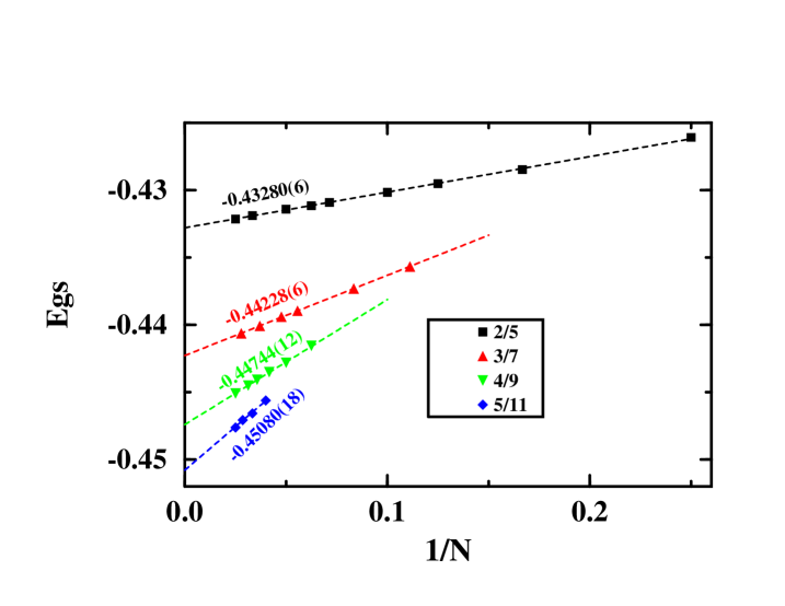
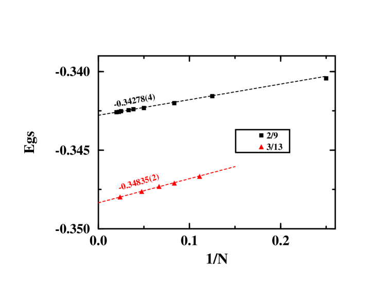
FIG. 1.: Ground state energy of various FQHE states as a function of the number of particles, $N$.

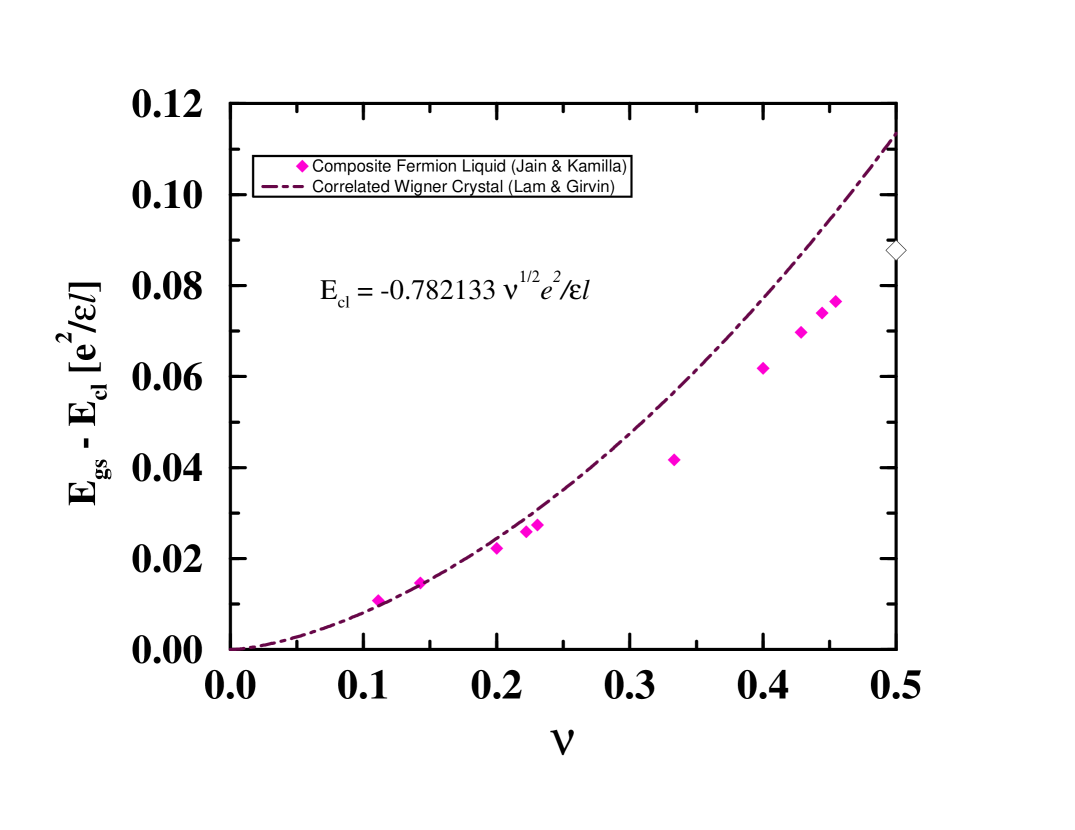
FIG. 2.: The energy of the liquid FQHE states and the correlated WC state. The WC energy is taken from [35]. Only the quantum correction to the energy of the classical ground state (a two-dimensional Wigner crystal with triangular symmetry) is shown, where $E_{cl}=-0.782133\sqrt{\nu}$ $e^{2}/\epsilon l$. The open diamond on the right vertical axis is our estimate of the CF ground state energy at $\nu=1/2$, $(E_{gs,1/2}-E_{cl}=0.0877(2)e^{2}/\epsilon l)$ obtained by extrapolating the energies of the $n/(2n+1)$ CF states. Also note that the energy of the CF liquid is shown only at the special $n/(2pn+1)$ filling factors; the full curve will have cusps at these points.

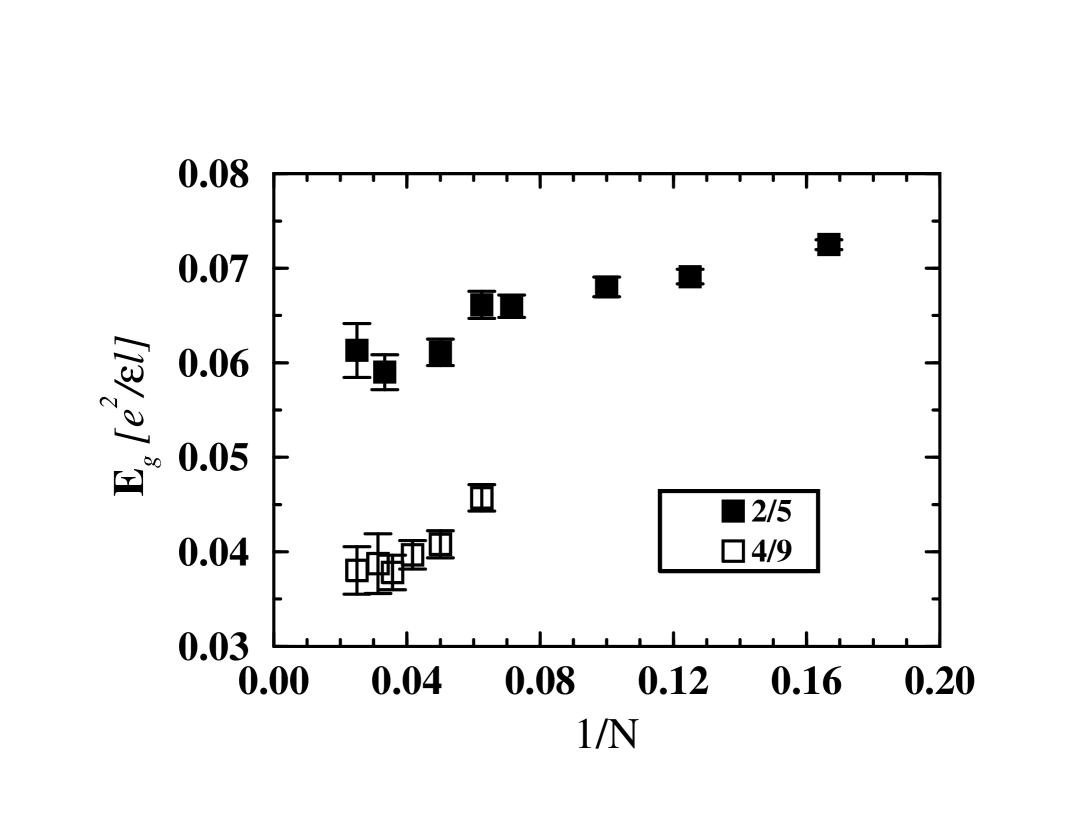
FIG. 3.: $N$ dependence of the “corrected” gap for 2/5 and 4/9.

FIG. 4.: Thermodynamic values of the gaps plotted as a function of $1/(2n+1)$. The results for the 1/3 gap are taken from Ref.[14]. The straight line is obtained by a chi-square fit, given by $E_{g}=0.000(5)+0.316(21)(2n+1)^{-1}$.

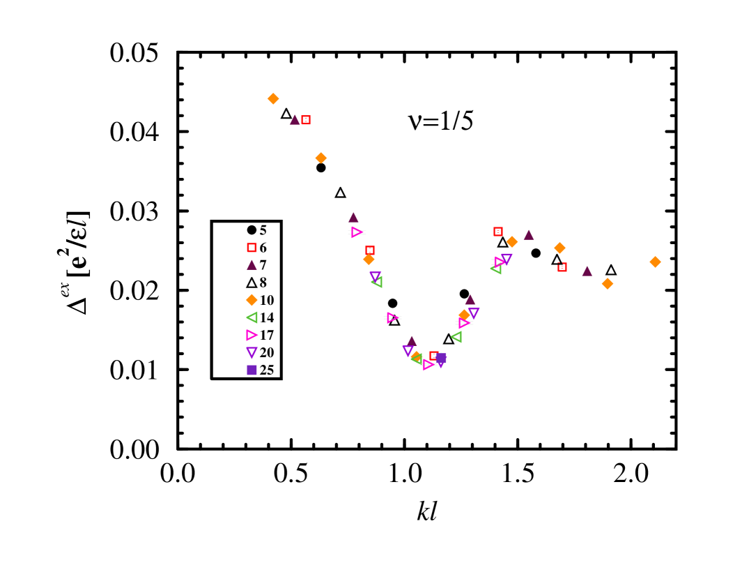
FIG. 5.: Exciton dispersions for FQHE states at $\nu=$ 1/5 for systems with several sizes, with $N$ shown on the figures. All curves assume zero thickness. The error bars are shown explicitly whenever they exceed the sizes of the symbols.

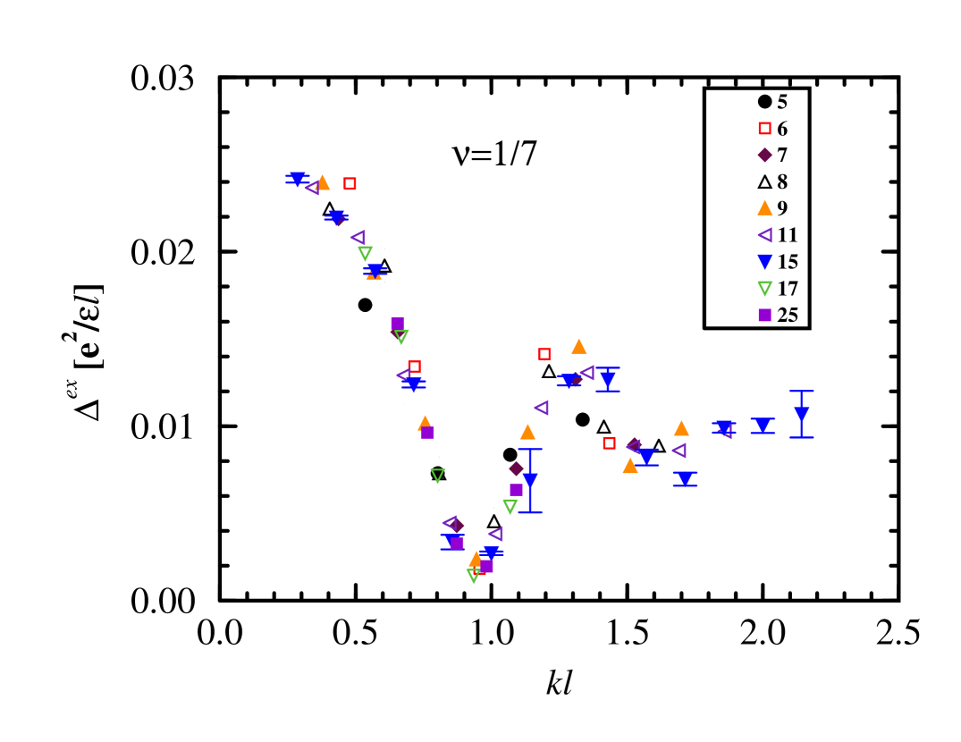
FIG. 6.: Same as in 5 for $\nu=1/7$.

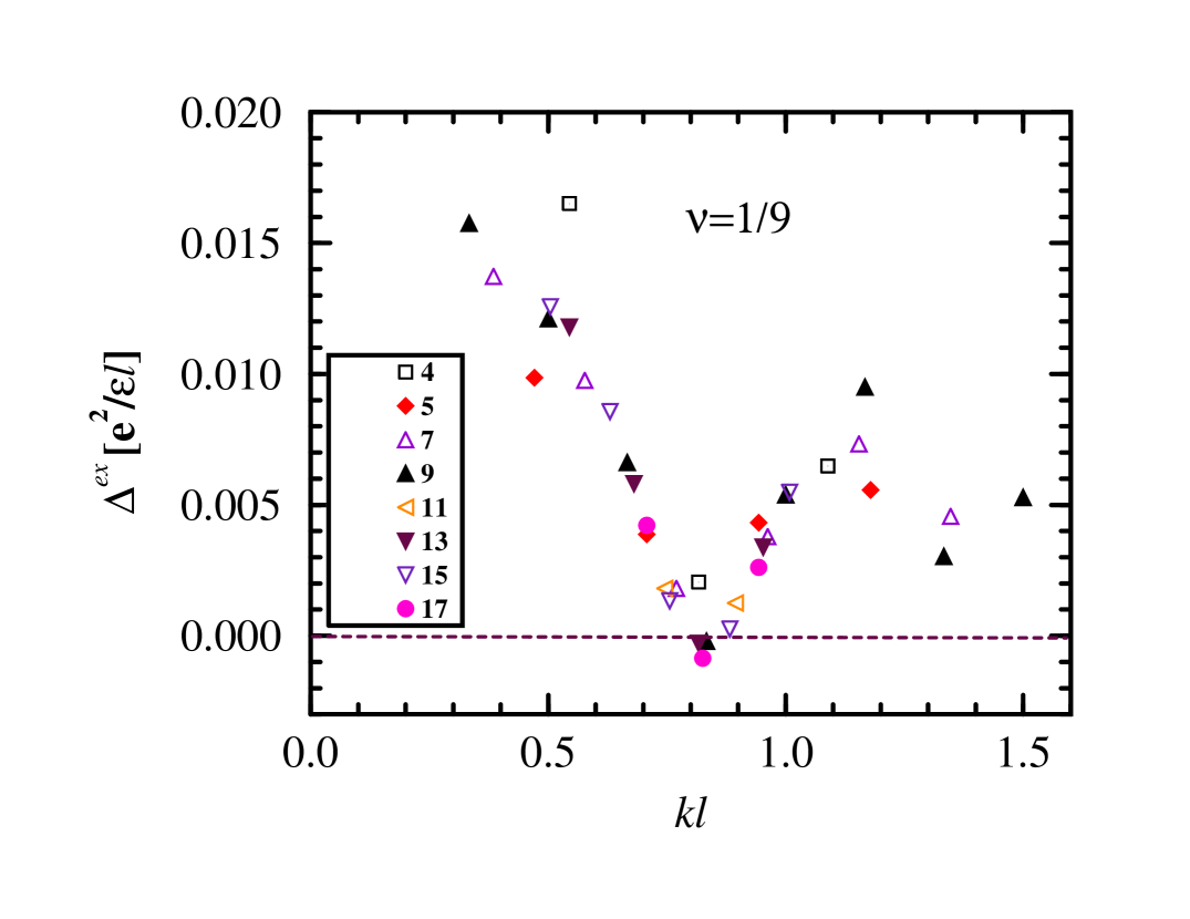
FIG. 7.: Same as in 5 for $\nu=1/9$.

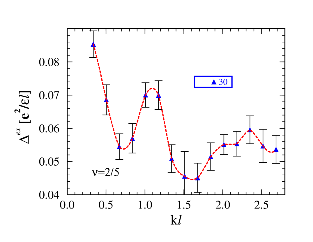
FIG. 8.: Exciton dispersions for $\nu=$ 2/5 for $N=30$. The dashed line is a guide to the eye.

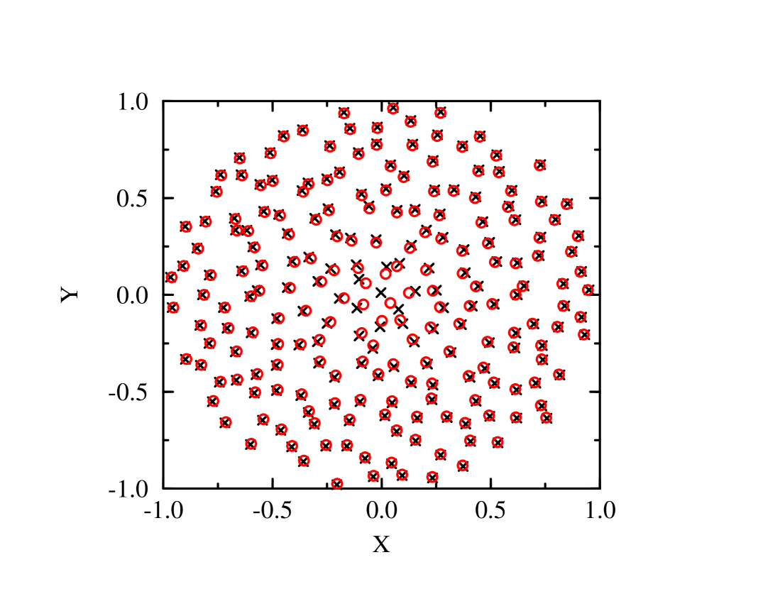
FIG. 9.: Positions of zeros (dots) of $F_{1}[z,\{z_{j}\}]$ for a given configuration of $z_{j}$ (crosses) for $N=200$. The other electrons ($z_{j}$) are taken to be in a reasonably probable configuration in the presence of a repulsive interaction. A defect is seen near the origin.

FIG. 10.: The empty circles show the exact ground state energy of seven interacting electrons confined to the lowest LL in the angular momentum $M$ sector obtained by an exact diagonalization of the Coulomb Hamiltonian. The filled triangles give the independent-defect-approximation for the energy of composite fermions in $M^{CF}$ state, $N_{D}E_{D}$, where $N_{D}$ is the minimum number of defects at $M^{CF}$ and $E_{D}$ is the energy of a single defect, chosen to be $E_{D}=0.125e^{2}/\epsilon\l$ to obtain the best fit (also, an arbitrary overall constant has been added to the defect energy). The filled dots show the Coulomb energies, evaluated by Monte Carlo. The configurations of the compact CF states are indicated on the figure in sequential order. The wave functions of these states contain no adjustable parameters. The lines are a guide to the eye

REFERENCES

- [1] See for a review, Perspectives in Quantum Hall Effects, edited by S. Das Sarma and A. Pinczuk (Wiley, New York, 1996).
- [2] J.K. Jain, Phys. Rev. Lett. 63, 199 (1989); Phys. Rev. B 41, 7653 (1990); Science 266, 1199 (1994).
- [3] R.R. Du, H.L. Stormer, D.C. Tsui, L.N. Pfeiffer, and K.W. West, Phys. Rev. Lett. 70, 2944 (1993); H.C. Manoharan, M. Shayegan, and S.J. Klepner, Phys. Rev. Lett. 73, 3270 (1994).
- [4] B.I. Halperin, P.A. Lee, and N. Read, Phys. Rev. B 47, 7312 (1993).
- [5] R.L. Willett et al., Phys. Rev. Lett. 71, 3846 (1993); W. Kang et al., ibid. 71, 3850 (1993); V.J. Goldman et al., ibid. 72, 2065 (1994); J.H. Smet et al., ibid. 77, 2272 (1996).
- [6] X.G. Wu, G. Dev, and J.K. Jain, Phys. Rev. Lett. 71, 153 (1993).
- [7] R.R. Du, A.S. Yeh, H.L. Stormer, D.C. Tsui, L.N. Pfeiffer and K.W. West, Phys. Rev. Lett. 75, 3926 (1995); H.L. Stormer, W. Kang, S. He, R.R. Du, A.S. Yeh, D.C. Tsui, L.N. Pfeiffer, K.W. Baldwin, K.W. West, Physica B 227, 164 (1996); R.R. Du, A.S. Yeh, H.L. Stormer, D.C. Tsui, L.N. Pfeiffer and K.W. West, Surf. Science, vol. 361-362, 26 (1996).
- [8] G. Dev and J.K. Jain, Phys. Rev. Lett. 69, 2843 (1992); M. Kasner and W. Apel, Phys. Rev. B 48, 11435 (1993); X.G. Wu and J.K. Jain, Phys. Rev. B 51, 1752 (1995).
- [9] E.H. Rezayi and N. Read, Phys. Rev. Lett. 72, 900 (1994).
- [10] M.P. Nightingale and C.J. Umrigar, Recent Advances in Quantum Monte Carlo Methods, edited by W.A. Lester (World Scientific Publishing, Singa pore, 1997).
- [11] N. Trivedi and J.K. Jain, Mod. Phys. Lett. B 5, 503 (1991); R.K. Kamilla and J.K. Jain, Phys. Rev. B, in print.
- [12] S. He, S.H. Simon and B.I. Halperin, Phys. Rev. B 50, 1823 (1994).
- [13] G. Fano, F. Ortolani, and E. Colombo, Phys. Rev. B 34, 2670 (1986).
- [14] N.E. Bonesteel, Phys. Rev. B 51, 9917 (1995), and private communication.
- [15] R.K. Kamilla, X.G. Wu, and J.K. Jain, Phys. Rev. Lett. 76, 1332 (1996).
- [16] J.K. Jain and R.K. Kamilla, Phys. Rev. B, 55, R4895 (1997).
- [17] R.K. Kamilla and J.K. Jain, unpublished.
- [18] F.C. Zhang and S. Das Sarma, Phys. Rev. B 33, 2903 (1986); D. Yoshioka, J. Phys. Soc. Jpn. 55, 885 (1986).
- [19] D. Yoshioka, J. Phys. Soc. Jpn. 53, 3740 (1984); X. Zhu and S.G. Louie, Phys. Rev. Lett. 70, 339 (1993) Rodney Price and S. Das Sarma, Phys. Rev. B, in print.
- [20] F.C. Zhang and S. Das Sarma, Phys. Rev. B 33, 2903 (1986).
- [21] A. Lopez and E. Fradkin, Phys. Rev. B 47, 7080 (1993); S.H. Simon and B.I. Halperin, Phys. Rev. B 48, 17368 (1993); D.H. Lee and S.C. Zhang, Phys. Rev. Lett. 66, 1220 (1991).
- [22] A. Stern and B.I. Halperin, Phys. Rev. B 52, 5890 (1995).
- [23] T.T. Wu and C.N. Yang, Nucl. Phys. B 107, 365 (1976); T.T. Wu and C.N. Yang, Phys. Rev. D 16, 1018 (1977).
- [24] F.D.M. Haldane, Phys. Rev. Lett. 51, 605 (1983).
- [25] E.P. Wigner, Phys. Rev. 46, 1002 (1934).
- [26] C.C. Grimes and G. Adams, Phys. Rev. Lett. 42, 795 (1979).
- [27] A. Pinczuk et al., Phys. Rev. Lett. 70 3983, 1993; H.D.M. Davies et al., preprint.
- [28] C.J. Mellor et al., Phys. Rev. Lett. 74, 2339 (1995).
- [29] N. d’Ambrumenil and R. Morf, Phys.Rev. 40, 6108 (1989).
- [30] R.B. Laughlin, Phys. Rev. Lett. 50, 1395 (1983).
- [31] R. Morf, N. d’Ambrumenil and B.I. Halperin, Phys. Rev. B 34, 3037 (1986).
- [32] S.M. Girvin, A.H. MacDonald and P.M. Platzman, Phys. Rev. Lett. 54 581, 1985; Phys. Rev. B 33, 2481 (1986).
- [33] U. Girlich and M. Hellmund, Phys. Rev. B 49, 17488 (1994); M. Kasner and W. Apel, ibid. 48, 11435 (1993).
- [34] D. Ceperley, G.V. Chester, M.H. Kalos; Phys. Rev. B 16, 3081 (1977); S. Fahy, X.W. Wang, and S.G. Louie, Phys. Rev. B 42, 3503 (1990).
- [35] P.K. Lam and S.M. Girvin, Phys. Rev. B 30, 473 (1984).
- [36] See, for example, G. Fano, F. Ortolani, and E. Tosatti, Il Nuovo Cimento D 9, 1337 (1987).
- [37] See, for example, G. Oritz, D.M. Ceperley, and R.M. Martin, Phys. Rev. Lett. 71, 2777 (1993).
- [38] V. Melik-Alaverdian and N.E. Bonesteel, Phys. Rev. B 52, R17032 (1996).
- [39] L. Bonsall and A.A. Maradudin, Phys. Rev. B 15, 1959 (1977).
- [40] V.J. Goldman, M. Shayegan, and D.C. Tsui, Phys. Rev. Lett. 61, 881 (1988); T. Sajoto et al., Phys. Rev. B 41, 8449 (1990).
- [41] P.M. Platzman and R. Price, Phys. Rev. Lett. 70, 3487 (1993).
- [42] P.M. Platzman and S. He, Phys. Rev. B 49, 13674 (1994).
- [43] J.N. Ginocchio and W.C. Haxton [Phys. Rev. Lett. 77, 1568 (1996)
- [44] J.K. Jain and T. Kawamura, Europhys. Lett. 29, 321 (1995); T. Kawamura and J.K. Jain, J. Phys. Cond. Matter 8, 2095 (1996); C.W.J. Beenakker and B. Rejaei, Physica B 189, 147 (1993).
- [45] J.K. Jain, Comments Cond. Mat. Phys. 16, 307 (1993).
- [46] S.M. Girvin and T. Jach, Phys. Rev. B 29, 5617 (1984).