Tunneling in quantum wires I: Exact solution of the spin isotropic case.

Abstract

We show that the problem of impurity tunneling in a Luttinger liquid of electrons with spin is solvable in the spin isotropic case ($g_{\sigma}=2$, $g_{\rho}$ arbitrary). The resulting integrable model is similar to a two channel anisotropic Kondo model, but with the impurity spin in a “cyclic representation” of the quantum algebra $su(2)_{q}$ associated with the anisotropy. Using exact, non perturbative techniques we study the RG flow, and compute the DC conductance. As expected from the analysis of Kane and Fisher we find that the IR fixed point corresponds to two separate leads. We also prove an exact duality between the UV and IR expansions of the current at vanishing temperature.

I Introduction.

Quantum impurity problems have attracted constant attention recently. The reason is, that the underlying physics is highly non trivial, that the models are manageable technically despite the presence of very strong interactions, and that there are many practical/experimental applications. The latter include the Kondo effect, quantum dots, dissipative quantum mechanics, impurity tunneling in fractional quantum Hall devices and in one dimensional quantum wires.

The physical variables are usually the temperature, the external field, the bulk interactions, the nature of the impurity (which can either be a charge or spin impurity), and the way it is coupled to the bulk degrees of freedom. A standard approach to computing physical quantities in these models would be to use perturbation theory in the bulk-impurity coupling for example. This perturbative expansion is most of the time done around the UV fixed point, and usually leads to limited results. Since all the problems of interest are essentially one dimensional (or can be reformulated as such), more powerful methods can however be used. For instance, in recent years, a conformal field theory description has allowed a much better understanding of the fixed points and their vicinity [1].

Another method, which is a priori less general, is the use of quantum integrability, pioneered in the study of the Kondo problem [2]. Integrability is a powerful, non perturbative tool, which is not limited to the vicinity of the fixed points but allows a complete description of the properties all the way along the renormalisation group flow, from the UV to the IR fixed points. Technical difficulties have for a long time restricted the use of integrability to the computation of thermodynamic, equilibrium properties. However, recent progress, in particular in the understanding of form factors [3] and integrable description of conformal field theories [4, 5], have also made possible the computation of dynamical, out of equilibrium properties for many quantum impurity problems [6, 7].

A still open challenge in that field is the problem of a single (charge) impurity in a one dimensional quantum wire, where the electrons are described by a Luttinger liquid with charge and spin degrees of freedom. This problem was studied using the renormalisation group and perturbation theory by Kane and Fisher [8] and Furusaki and Nagaosa [9]. There, a complete picture of the flows generated by the RG was obtained in terms of the “$g$” factors, $g_{\rho}$ and $g_{\sigma}$, describing the interaction of bulk charge and spin degrees of freedom. The existence of tentalizing new fixed points, which would be partly transmitting and partly reflecting, was in particular conjectured. Steps were taken to identify these fixed points using conformal field theory [10], but the problem remains open.

In this paper, we are addressing this impurity problem from the point of view of integrability. The case of an impurity in a spinless electron gas could be mapped on the boundary sine-gordon model [6], which is a completely integrable quantum field theory [11], formally analogous to the anisotropic Kondo problem, but with the impurity spin in a cyclic representation of the quantum algebra $su(2)_{q}$ [12]. Here, we show that the case of electrons with spin maps, when $g_{\sigma}=2$, onto a model analogous to the anisotropic two channel Kondo model, again with the impurity spin chosen in a cyclic representation of the quantum algebra $su(2)_{q}$. This allows us to compute the relevant physical properties.

II The model, integrability, and the $S$ matrix.

In order to fix notations, let us repeat some of the basic definitions in [8]. In the one dimensional Luttinger liquid, bosonisation of the fermionic operators is accomplished via

$$\psi_{\mu}^{\dagger}\simeq\sum_{n\ odd}e^{in[\sqrt{\pi}\Theta_{\mu}+k_{F}x]}e^{i\sqrt{\pi}\phi_{\mu}(x)},$$ (1)

with $\mu=\uparrow,\downarrow$. The fields $\phi_{\mu}$ and $\Theta_{\mu}$ have commutation relations

$$[\phi_{\mu}(x),\Theta_{\mu^{\prime}}(x^{\prime})]=i\delta_{\mu,\mu^{\prime}}\theta(x-x^{\prime})$$ (2)

from which we can devise two different representations of the Luttinger liquid (our conventions follow [8]). Here, we will work in the so called $\Theta$-representation. Changing basis to the charge and spin degrees of freedom

$$\Theta_{\rho}=\Theta_{\uparrow}+\Theta_{\downarrow},\ \ \Theta_{\sigma}=\Theta_{\uparrow}-\Theta_{\downarrow},$$ (3)

we obtain the action

$$S = S_{\rho}+S_{\sigma}$$ (4)

$$= \int dxdy\frac{1}{2g_{\rho}}[(\partial_{x}\Theta_{\rho})^{2}+(\partial_{y}\Theta_{\rho})^{2}]+\frac{1}{2g_{\sigma}}[(\partial_{x}\Theta_{\sigma})^{2}+(\partial_{y}\Theta_{\sigma})^{2}].$$ (5)

where $y$ is the imaginary time, the spin and charge velocities have been normalised such that $v_{\sigma}=v_{\rho}=1$. In this convention, the g-factors have value $g_{\sigma}=g_{\rho}=2$ for a non-interacting system. The case of quantum wires with $SU(2)$ symmetry corresponds to $g_{\sigma}=2$.

The electric and magnetic conductances of this system follow directly from Kubo’s formula

$$G_{\rho/\sigma}=\frac{e^{2}}{h}g_{\rho/\sigma}.$$ (6)

As discussed in [13], this formula might not always be physically relevant, because of the coupling to the reservoirs. It has been proposed that $G_{\rho}=2\frac{e^{2}}{h}$ might always hold, whatever the interactions in the quantum wire. Of course, this does not mean that the scattering through the impurity will be trivial in that case; it will indeed, still be controlled by the action written above, the only difference being in the meaning of the “applied voltage”. Here, we will simply follow [8] for uniformity of notations. Physical results for different reservoirs configurations can be recovered by rescaling the voltage.

In the presence of a charge impurity at the origin $x=0$, the hamiltonian gets an additional piece

$$\delta H=\int dxV(x)(\psi^{\dagger}_{\uparrow}\psi_{\uparrow}+\psi^{\dagger}_{\downarrow}\psi_{\downarrow}).$$ (7)

Here $V(x)$ is a potential which has essentially zero measure outside $x=0$. Under the bosonisation rules sketched at the beginning, this leads to the change of action

$$\delta S=\lambda\int dy\cos\sqrt{\pi}\Theta_{\rho}\cos\sqrt{\pi}\Theta_{\sigma},$$ (8)

where $\lambda\simeq V(2k_{F})$. In the physical case, there is no apparent symmetry that allows us to restrict to the action (8) - the most general form of the perturbation is

$$\delta S=\int dy\sum_{n_{\rho},n_{\sigma}\atop n_{\rho}+n_{\sigma}\ even}\frac{\lambda_{n_{\rho},n_{\sigma}}}{4}e^{i\sqrt{\pi}(n_{\rho}\Theta_{\rho}+n_{\sigma}\Theta_{\sigma})}$$ (9)

where the $\lambda$’s are real couplings. The renormalisation group equations read at first order

$$\frac{d\lambda_{n_{\rho},n_{\sigma}}}{dl}=\left(1-\frac{n_{\rho}^{2}}{4}g_{\rho}-\frac{n_{\sigma}^{2}}{4}g_{\sigma}\right)\lambda_{n_{\rho},n_{\sigma}}.$$ (10)

As mentioned before, in this paper we restrict to the case $g_{\sigma}=2$, which is the one relevant for physical quantum wires with unbroken $SU(2)$ spin symmetry. Then, beside the perturbation with $n_{\rho}=n_{\sigma}=1$, the operators $n_{\rho}=2,n_{\sigma}=0$ is relevant for $g_{\rho}<1$. The operator with $n_{\sigma}=2,n_{\rho}=0$ is always irrelevant. We will thus further restrict in the following to the (probably not physically relevant) case where only $\lambda_{11}\neq 0$ or the case where $g_{\rho}>1$, so we have to take into account the term $\lambda_{11}$ only, which we simply call $\lambda$ in what follows.

In [6], the equivalent problem for spinless electrons was exactly solved. The solution required a folding to transform the impurity problem into a boundary problem, and then used recent results on boundary integrable quantum field theories [11] together with the massless scattering approach. The same folding can easily be accomplished in the problem with spin. First, it is convenient to rescale the fields, writing the action as

$$S = S_{\rho}+S_{\sigma}+\lambda\int dy\cos\sqrt{\pi g_{\rho}}\Theta_{\rho}\cos\sqrt{2\pi}\Theta_{\sigma}$$ (11)

$$S_{\mu} = \int dxdy\frac{1}{2}[(\partial_{x}\Theta_{\mu})^{2}+(\partial_{y}\Theta_{\mu})^{2}].$$ (12)

We then introduce odd and even fields

$$\Theta^{e}_{\mu} = \frac{1}{\sqrt{2}}[\Theta_{\mu,L}(x,y)+\Theta_{\mu,R}(-x,y)]$$ (13)

$$\Theta^{o}_{\mu} = \frac{1}{\sqrt{2}}[\Theta_{\mu,L}(x,y)-\Theta_{\mu,R}(-x,y)].$$ (14)

With this, the interaction at $x=0$ involves only the even fields which have Neumann boundary conditions. The odd fields, having Dirichlet boundary conditions, completely decouple and do not interact. Also, the even field, as defined above, is left moving and we can “fold” using

$$\theta_{\mu,L} = \Theta^{e}(x+y),\ x<0$$ (15)

$$\theta_{\mu,R} = \Theta^{e}(-x,y),\ x<0.$$ (16)

We can now express everything in terms of the fields $\theta$ which is defined on the negative axis, the action becomes

$$S = S_{0}+{\cal B}$$ (17)

$$= \int_{-\infty}^{0}dx\int dy\ \frac{1}{2}\sum_{\mu=\sigma,\rho}[(\partial_{x}\theta_{\mu})^{2}+(\partial_{y}\theta_{\mu})^{2}]+\lambda\int dy\cos\sqrt{\frac{\pi g_{\rho}}{2}}\theta_{\rho}(0)\cos\sqrt{\pi}\theta_{\sigma}(0).$$ (18)

The next step in [6] was to use the integrability of the corresponding boundary quantum field theory - the boundary sine-Gordon model (BSG). In the present case with spin, the problem, involving two fields, is a priori more complicated. Indeed it is unlikely that the problem is soluble for general values of $g_{\rho},g_{\sigma}$. However, in the case $g_{\sigma}=2$, the problem can be solved, as we now demonstrate.

The trick to solve a boundary problem such as the one under consideration here, is to introduce a more general integrable problem with both bulk and boundary perturbations. The bulk term is chosen such that the theory remains integrable thus defining a basis of quasiparticles bulk excitations. These excitations are interacting through an elastic, two particles $S$ matrix derived from the constraints of unitarity, crossing-symmetry and the Yang-Baxter equation [14]. Since the theory with boundary is also integrable, there are also strong constraints on the boundary reflection matrix $R$ leading to a very simple scattering of these quasiparticles at the boundary. When one lets the bulk coupling go to zero, these become massless quasiparticles which scatter in a simple way at the boundary. Taking the massless limit is by now a standard procedure and has been discussed in [15, 16].

In our case, we need to find the appropriate bulk perturbation for the problem. The first natural idea to handle (17) is to introduce as a bulk perturbation

$$S_{B}=\Lambda\int_{-\infty}^{0}dx\int dy\ \cos 2\sqrt{\pi}\theta_{\sigma}\cos\sqrt{2\pi g_{\rho}}\theta_{\rho}$$ (19)

Note the doubling of the cosine’s arguments compared with (17): this is because, quite generally, an integrable perturbation of the form $f(\theta^{L})f(\theta^{R})$ corresponds to an integrable perturbation $f(\theta^{R})$ at the boundary. Here the function $f$ is an exponential (to make the action real, appropriate combinations of exponentials were taken), and, using Neumann boundary conditions, we wrote $\cos\theta(0)=\cos 2\theta^{R}(0)$. The problem (19) is however not integrable for generic values of $g_{\rho}$ (integrable sub-varieties have been identified in [17, 18, 19] and will be the subject of a sequel to this paper), so this approach is not satisfactory. Fortunately, we can introduce another bulk perturbation,

$$S_{B}=\Lambda\int_{-\infty}^{0}dx\int dy\ \cos 2\sqrt{\pi}\theta^{L}_{\sigma}\cos 2\sqrt{\pi}\theta^{R}_{\sigma}\cos\sqrt{2\pi g_{\rho}}\theta_{\rho}$$ (20)

This corresponds to the function $f$ being a cosine function. This problem is actually well known to be integrable. To see this, we can refermionize the $\theta_{\sigma}$ part. The term $\cos 2\sqrt{\pi}\theta^{R}_{\sigma}$ being the sum of a an exponential and its conjugate becomes now a Majorana fermion, so we have, equivalently,

$$S_{B}=\Lambda\int_{-\infty}^{0}dx\int dy\ \Psi\bar{\Psi}\cos\sqrt{2\pi g_{\rho}}\theta_{\rho}$$ (21)

while the free part can be written as a free bosonic hamiltonian, plus the sum of two decoupled free Majorana fermions, only one of them appearing into the perturbation

$$S_{0}=\int_{-\infty}^{0}dx\int dy\ \frac{1}{2}[(\partial_{x}\theta_{\rho})^{2}+(\partial_{y}\theta_{\rho})^{2}]+\Psi\bar{\partial}\Psi-\bar{\Psi}\partial\bar{\Psi}+\chi\bar{\partial}\chi-\bar{\chi}\partial\bar{\chi}.$$ (22)

Factoring out the other fermion ($\chi$), we end up with a standard integrable $c=3/2$ analog of the sine-Gordon model [33]. The boundary perturbation is also integrable. In terms of fermions, it can be written as

$$\lambda\int dy\ \cos\sqrt{\frac{\pi g_{\rho}}{2}}\theta_{\rho}(0)\left[\Psi(0)+\bar{\Psi}(0)\right]a(y)+{1\over 2}\int dy\left[\Psi\bar{\Psi}(0)+a\dot{a}\right].$$ (23)

The last part simply enforces appropriate UV boundary conditions . The quantum operator $a$ anticommutes with the fermions, and satisfies $a^{2}=1$ (see [20] for a detailed discussion of bosonization in the presence of a boundary).

In the bulk, the theory can be shown to be integrable by exhibiting a set of non-local conserved currents

$$J^{\pm}=\Psi e^{\pm i\theta^{R}_{\rho}/\sqrt{2\pi g_{\rho}}},\ \bar{J}^{\pm}=\overline{\Psi}e^{\pm i\theta^{L}_{\rho}/\sqrt{2\pi g_{\rho}}}$$ (24)

These currents in turn define conserved charges with $\widehat{su(2)}_{\hat{q}}$ commutation relations. They commute with the charges constructed from the following local currents

$$G=\Psi\partial\theta_{\rho},\ \ \overline{G}=\overline{\Psi}\ \overline{\partial}\theta_{\rho}$$ (25)

which are also conserved by the perturbation. Requiring that these symmetries are realized on the asymptotic states of the theory leads to a bulk $S$ matrix factorized into a a $\widehat{su(2)}_{\hat{q}}$, sine-Gordon type part describing the scattering of a doublet, $S_{ud}$, and a supersymmetric part, which is basically a kink $S$ matrix with 3 vacua [30].

It must be mentioned here that there are some subtle issues regarding the integrability of the previous field theory - for simplicity we discuss only the bulk case here, the boundary case being quite similar. Although naive power counting following the arguments of [21] suggests that the theory is integrable at any order, the fact that the fermions have integer dimension makes the problem more complicated. It is generally believed that the integrable theory requires an additional term of the form $\Lambda^{2}\cos 2\sqrt{2\pi g_{\rho}}\phi$, as can be checked in the semiclassical case [22], or by imposing $N=1$ supersymmetry. The universal properties of the model (21) are the same as the one with this additional coupling. Indeed, consider for instance the computation of the free energy perturbatively. If $a$ is the short distance cut-off, its expansion involves the coupling $\Lambda(R/a)^{{1\over 2}-2g_{\rho}}$ for every insertion of the first operator, and the coupling $\Lambda^{2}(R/a)^{1-8g_{\rho}}$ for every insertion of the second. For $g_{\rho}$ positive, the integrals are divergent. They could either be rendered finite by dimensional regularization (akin to taking $g_{\rho}$ negative), or by using the cut-off. In the latter case, the divergent part will only contribute to the regular, bulk part (see eg [23]). Writing the free energy per unit length $f=f_{reg}-T\hat{f}$, letting $T=1/R\to 0$ and $\Lambda\to 0$ such that $x\equiv\Lambda R^{1-2g_{\rho}}$ remains finite, we obtain a function $\hat{f}(x)$ determined fully by insertions of the first operator, not of the second one.

In fact one can avoid the appeal to this discussion of the bulk integrable theory, and $N=1$ supersymmetry, by addressing the problem from the two channel Kondo model point of view. It is well established that the anisotropic Kondo problem is integrable for any number of channels and impurity spin; the case at hand corresponds simply to a particular impurity spin - a cyclic representation of the quantum algebra $su(2)_{q}$. In particular, for the anisotropic two channel Kondo model, the S-matrix of the excitations in the bulk is precisely the one mentionned above ($S_{ud}\otimes S_{kink}$). This identification in addition gives the impurity S-matrix immediately - this is discussed in more details in appendix B.

Recall that the solution of the massless problem proceeds by first describing the bulk problem in terms of massless relativistic excitations - the limit $\Lambda\to 0$ of the excitations of (21). The basic massless particles are then either right or left moving, with dispersion relation $e=p$ ($e=-p$), and they have a spin quantum number and a kink quantum number. We denote them by the doublet $(u_{a,a\pm 1},d_{a,a\pm 1})$. The label $a$ denotes one of the 3 possible vacua; a kink connects adjacent vacua, and is thus designated by a pair of labels (see figure 1). We use for the kinematic properties of these basic particles the same parametrization, $e=me^{\theta}$, where $m$ has the dimension of a mass, although the theory is massless.

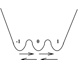
FIG. 1.: Structure of the vacuas for the RSOS sector.

The particles have factorized scattering, with trivial $LR$ scattering. The LL and RR scattering are described by the bulk S matrix with tensor product structure

$$S=S_{ud}\otimes S_{kink}$$ (26)

Here $S_{ud}$ is the usual soliton-antisoliton sine-Gordon S-matrix, corresponding to the coupling ${\beta^{2}\over 8\pi}\equiv{\gamma\over\gamma+1}$, ie a quantum group symmetry with deformation parameter $q=-e^{-i\pi/\gamma}$, where ${g_{\rho}\over 4}={\gamma\over 2(\gamma+2)}$, so the total dimension of the boundary perturbation (using that $g_{\sigma}=2$) is $d={1\over 2}+{\gamma\over 2(\gamma+2)}={\gamma+1\over\gamma+2}$. The kink S-matrix is the well known Restricted Solid on Solid S-matrix for a model with three vacua. There may also be bound states, depending on the value of $\gamma$. There are no such bound states if $\gamma$ is larger than one. When $\gamma$ is smaller than one, there are $n$ of them, where $n$ is the integer part of $1/\gamma$.

The integrability of the model with boundary interaction translates into the fact that massless particles are reflected with no particle production, in a way described by a reflection matrix $R$, solution of the boundary Yang-Baxter equation. By analogy with the higher spin two-channel Kondo model (see appendix B), we find

$$R=R_{u,d}\otimes 1$$ (27)

where $R_{u,d}$ is the reflection matrix of the boundary sine-Gordon problem at the foregoing coupling $\beta$. It is enough for our purpose to recall the physical amplitudes

$$\left|R_{u}^{u}\right|^{2}={1\over 1+e^{-{2\over\gamma}(\theta-\ln T_{B})}},\ \left|R_{u}^{d}\right|^{2}=1-\left|R_{u}^{u}\right|^{2}$$ (28)

Here $T_{B}$ is an energy scale related with the coupling $\lambda$ by $T_{B}\propto\lambda^{-1/(d-1)}\propto\lambda^{\gamma+2}$. Physical quantities to be discussed below will be expressed in terms of the squares of R-matrix elements, and therefore expand in powers of $T_{B}^{2/\gamma}$. On the other hand, these quantities expand in powers of the square of the amplitude in front of the leading irrelevant operator determining the approach to the IR fixed point. If the IR fixed point is approached along $\mu O$, with $O$ of dimension $d$, then $\mu$ has dimension $1-d$. Hence we find $2(d-1)={2\over\gamma}$ or $d={1\over\gamma}+1={\gamma+1\over\gamma}={1\over 2}+{\gamma+2\over 2\gamma}={1\over g_{\sigma}}+{1\over g_{\rho}}$. Following the discussion in [8], this indicates that the IR fixed point corresponds to “disconnected leads”, as expected in that domain of the parameters.

III DC transport properties

The whole logic of [6] can now be implemented. To compute DC properties, it is enough to treat the massless particles as free ones from the point of view of impurity scattering, ie use a Landauer Büttiker type formula. The massless particles are quantized using TBA equations. The system of equations, for $\gamma$ an integer, is, setting $\rho_{j}^{h}/\rho_{j}=e^{\epsilon_{j}}$

$$\epsilon_{j}(\theta,V/T)=\delta_{j,2}{me^{\theta}\over T}-K\star\sum_{k}N_{jk}\ln\left[1+e^{\mu_{k}}e^{-\epsilon_{k}(\theta,V/T)}\right].$$ (29)

where the kernel $K(\theta)\equiv{1\over(2\pi\cosh\theta)}$, and $N_{jk}$ is the incidence matrix of the following diagram (which is found by “gluing” the RSOS and the non-diagonal sine-Gordon TBA diagrams)

FIG. 2.: TBA diagram at zero temperature.

i.e. $N_{jk}=1$ if the nodes $j$ and $k$ are connected, and $0$ otherwise (in particular $N_{jj}=0$). The chemical potential vanishes, except for the end nodes, where $\mu=\pm(\gamma+1){V\over 2T}$, $V$ the applied voltage. Here, all the nodes but the one with $j=2$ correspond to pseudoparticles, which are necessary to diagonalize the S-matrix.

A Closed form solution at $T=0$

The simplest case is when $T=0$. Then, a Fermi sea of antisolitons is formed when a voltage is applied. All the scattering involves these antisolitons only, so the results can simply be derived for any value of $\gamma$. Introduce the quantity $\epsilon$, solution of

$$\epsilon(\theta)-\int_{-\infty}^{A}\Phi(\theta-\theta^{\prime})\epsilon(\theta^{\prime})d\theta^{\prime}={V\over 2}-{m\over 2}e^{\theta}$$ (30)

Here, $\Phi$ is a kernel with Fourier transform

$$\tilde{\Phi}(\omega)={1\over 4\cosh^{2}\pi\omega/2}+{1\over 2\cosh\pi\omega/2}{\sinh(\gamma-1)\pi\omega/2\over\sinh\gamma\pi\omega/2}$$ (31)

It is convenient to write it in the form

$$\tilde{\Phi}=1-{\sinh(\gamma+2)\pi\omega/2\over 4\cosh^{2}\pi\omega/2\sinh\gamma\pi\omega/2}$$ (32)

At zero temperature, $\epsilon(\theta)$ describes the excitation energy of the positively charged quasiparticles in the system which are the only ones filling the Fermi sea at $V\neq 0,T=0$. Taking a derivative of (30) we get the density of these quasiparticles

$$\rho(\theta)-\int_{-\infty}^{A}d\theta^{\prime}\ \rho(\theta^{\prime})\Phi(\theta-\theta^{\prime})=\frac{1}{2h}e^{\theta}.$$ (33)

The current then follows from a Boltzmann equation describing the one by one scattering of these charged excitation on the boundary. There are $\rho(\theta)d\theta$ such particles in $[\theta,\theta+d\theta]$ and the probability that a particle of type $\alpha$ is reflected as one of type $\alpha^{\prime}$ is $|R_{\alpha}^{\alpha^{\prime}}(\theta-\log(T_{B}))|^{2}$. This leads, following the arguments of [6] to the current

$$I(V,T_{B})=e\int_{-\infty}^{A}d\theta\ \rho(\theta)|R_{u}^{u}(\theta-\log(T_{B}))|^{2}.$$ (34)

Thus if we manage to determine $A$ and solve the linear integral equation for $\rho$ we get an exact evaluation for $I(V,T_{B})$. Since the integral equations are linear, this is possible by Wiener-Hopf techniques.

In the previous equations, $A$ is the Fermi rapidity defined by $\epsilon(A)=0$; it is the edge of the Fermi sea. $A$ can be determined, and the foregoing equations solved, by using a standard Wiener Hopf analysis. If we write $K(\theta)=\delta(\theta)-\Phi(\theta)$, we have

$$\tilde{K}(\omega)=\frac{1}{N(\omega)N(-\omega)},$$ (35)

with

$$N(\omega)=2\pi\sqrt{\frac{\gamma+2}{\gamma}}\frac{\Gamma(i(\gamma+2)\omega/2)e^{i\omega\Lambda}}{\Gamma(i\gamma\omega/2)\Gamma(1/2+i\omega/2)^{2}},$$ (36)

where $\Lambda$ is chosen to preserve the analyticity in the lower half plane. Here the conventions for the Fourier transforms are

$$g(\theta)=\int_{-\infty}^{\infty}\frac{d\omega}{2\pi}e^{-i\omega\theta}\tilde{g}(\omega),\ \ \tilde{g}(\omega)=\int_{-\infty}^{\infty}d\theta e^{i\omega\theta}g(\theta).$$ (37)

Then following exactly the same steps as in [6] we find the solution for the fourier transform of the density

$$\tilde{\rho}(\omega)=\frac{1}{2h}\frac{e^{(1+i\omega)A}}{(1+i\omega)}N(-i)N(\omega).$$ (38)

The excitation energy of the particles follows

$$\tilde{\epsilon}(\omega)e^{-i\omega A}=-i\frac{qV}{2}\frac{N(0)N(\omega)}{\omega}+\frac{ie^{A}}{2}\frac{N(-i)N(\omega)}{\omega-i}.$$ (39)

The condition $\epsilon(A)=0$ is equivalent to

$$\lim_{\omega\rightarrow\infty}\omega\tilde{\epsilon}(i\omega)e^{-i\omega A}=0,$$ (40)

which in turns gives the explicit value of the Fermi rapidity, $A$

$$e^{A}=eV\frac{N(0)}{N(-i)}.$$ (41)

We are then left with the evaluation of the current given in (34). After a few manipulations we get the exact expression

$$I(V,T_{B})=\frac{e}{2h}e^{A}N(-i)\int_{-\infty}^{A}d\theta\int_{-\infty}^{\infty}\frac{d\omega}{2\pi}\frac{e^{-i\omega\theta}}{(1+i\omega)}\frac{N(\omega)}{1+e^{-2/\gamma(\theta+A-\log T_{B})}}.$$ (42)

This can be expanded in powers of $V/T_{B}$ to get an IR expansion given by

$$I(V,T_{B}) = \frac{ee^{A}}{2h}N(-i)\sum_{n=1}^{\infty}(-1)^{n+1}\frac{N(-2in/\gamma)}{(1+2n/\gamma)}\left(\frac{e^{A}}{T_{B}}\right)^{2n/\gamma}$$ (43)

$$= 2\pi\frac{e^{2}V}{h}\sum_{n=1}^{\infty}(-1)^{n+1}\frac{\Gamma(2n/g_{\rho})}{(n-1)!\ \Gamma(\frac{1}{2}+\frac{n(2-g_{\rho})}{2g_{\rho}})^{2}[1+n(\frac{2-g_{\rho}}{g_{\rho}})]}\left(\frac{eV}{T_{B}^{\prime}}\right)^{n(2-g_{\rho})/g_{\rho}}$$ (44)

where we have reinstated the dependence on $g_{\rho}$ in the last expression and we have introduced the parameter

$$T_{B}^{\prime}=T_{B}\frac{2\pi}{2-g_{\rho}}$$ (45)

for convenience. We can also separate the integral over rapidities to get an expansion in the UV. After a few manipulations we get

$$I(V,T_{B})=\frac{e}{2h}N(-i)e^{A}PP\int\frac{d\omega}{2\pi}\frac{N(\omega)}{(1+i\omega)}\left\{\sum_{n=0}^{\infty}(-1)^{n+1}\frac{b^{n}}{2n/\gamma+i\omega}+\frac{\gamma}{2}\frac{b^{-i\omega\gamma/2}}{\sin(i\pi\omega\gamma/2)}\right\}$$ (46)

with $b=(T_{B}e^{-A})^{2/g_{\rho}}$. We integrate the first sum by closing the contour in the lower half plane and the second term by closing in the upper half plane. In the second term, the zeroes of $N(\omega)$ cancels the poles of $\sinh(\pi\omega\gamma/2)$ and the one at $\omega=i$, only the poles $\omega=2ni/(\gamma+2)$ with $n$ integer contribute. We get

$$I(V,T_{B})=\frac{e^{2}V}{h}g_{\rho}+\sum_{n=1}^{\infty}U_{n}\left(\frac{T_{B}^{\prime}}{eV}\right)^{n(1-g_{\rho}/2)},$$ (47)

with the coefficients

$$U_{n}=\frac{\pi}{2}\frac{e^{2}V}{h}g_{\rho}^{2}\frac{(-1)^{n}}{(n-1)!}\frac{\Gamma(ng_{\rho}/2)}{\Gamma(1/2-n(2-g_{\rho})/4)^{2}[1-n(2-g_{\rho})/2]},$$ (48)

where again we have reexpressed things in terms of $g_{\rho}$. From these two expressions we can check that there is an exact duality between the UV expansion and the IR expansion under the exchange $g_{\rho}\rightarrow 4/g_{\rho}$. This duality is more transparent through the relation

$$I(V,T_{B}^{\prime},g_{\rho})=\frac{e^{2}V}{h}g_{\rho}-\frac{g_{\rho}^{2}}{4}I(V,T_{B}^{\prime},4/g_{\rho}).$$ (49)

In order to make contact with perturbation theory, we need to find the relation between the boundary scale $T_{B}$ and $\lambda$. This is done in appendix B using a first order Keldysh computation.

B Conductance at finite temperature

To compute the conductance in the case $T\neq 0$ and $\gamma$ an integer is difficult. The reason is, that the bulk scattering is not diagonal in the soliton antisoliton basis, and the TBA equations are written, in fact, for quasiparticles with no definite charge. The transport equation of [12] becomes then ambiguous to use. In the case without spin, it was possible to conjecture a formula, based on limiting cases, that reproduced well numerical results, and later was established using more complicated functional relations. A similar conjecture in the present case would be

$$G={\gamma^{2}\over 2}\int{d\theta\over\cosh^{2}(\theta-\ln T_{B}/T)}\left[{1\over 1+e^{\epsilon_{\gamma+1}(\theta)}}-{1\over 1+e^{\epsilon_{\gamma+1}(\infty)}}\right]$$ (50)

It does go to zero in the infrared, as $T/T_{B}\to 0$. In the ultraviolet, when $T/T_{B}\to\infty$, it is easy to see that $G$ goes to $g_{\rho}$ as desired. This is because, in that limit, the only contribution to the integral comes from the region $\theta$ near infinity, where the $\epsilon$’s go to a constant, in particular, $e^{-\epsilon_{\gamma+1}(-\infty)}\to\gamma+1$ (while $e^{-\epsilon_{\gamma+1}(\infty)}\to\gamma-1$).

The case $\gamma=1/n$, $n$ an integer, belongs to the attractive regime of the sine-Gordon part of our scattering, and corresponds to the case with purely diagonal scattering. It is thus more favorable to study the conductance via the approach of [12]. However, while the attractive regime of the ordinary sine-Gordon model has been much studied, we are not aware of many such studies for the $N=1$ sine-Gordon model of interest here. The complete S-matrix was found in [31]. The TBA has never been written, as far as we know. We will present a detailed discussion of this problem elsewhere. Here, we content ourselves by giving the relevant equations and the corresponding conductance. The diagram looks as follows

FIG. 3.: TBA diagram at finite temperature.

The TBA equations have the form

$$\epsilon_{j}(\theta,V/T)=K*\sum_{k}N_{jk}\ln\left[1+e^{-\mu_{k}}e^{\epsilon_{k}(\theta,V/T)}\right]$$ (51)

with $K(\theta)={n\over 2\pi\cosh n\theta}$ and $j=3,\ldots,n+2$, $\mu_{n+1}=-\mu_{n+2}={V\over 2T}$, $\mu_{k}=0$ otherwise. In addition we have

$$\epsilon_{2}(\theta,V/T)=K*\left(\ln\left[1+e^{\epsilon_{3}}\right]-\ln\left[1+e^{-\epsilon_{1}}\right]\right)$$ (52)

and

$$\epsilon_{1}=-K*\ln\left[1+e^{\epsilon_{2}}\right]-K^{\prime}*\ln\left[1+e^{-\epsilon_{1}}\right]+\frac{e^{\theta}}{T}\frac{\sin\pi/2n}{\cos\pi/2n}.$$ (53)

Here we have

$$\tilde{K}={1\over 2\cosh\pi\omega/2n},\ \ \tilde{K^{\prime}}={\cosh(n-1)\pi\omega/2n\over 2\cosh\pi\omega/2n\cosh\pi\omega/2}$$ (54)

The other mass terms appear in the TBA in the form of asymptotic conditions:

$$\epsilon_{j}(\theta)\approx\frac{m_{j}}{T}e^{\theta}$$ (55)

where $m_{j}=2\sin{(j-1)\pi\over 2n}\,\,\,\,j>1$, $m_{n+1}=m_{n+2}=1$.

We can present, as a quick check of the validity of this TBA, a computation of the central charge of the theory. Setting $x\equiv e^{-\epsilon(-\infty)}$ we have the system

$${1\over x_{j}}=\prod_{k}\left(1+{1\over x_{k}}\right)^{N_{jk}/2}$$ (56)

supplemented by

$${1\over x_{2}}=\left(1+{1\over x_{3}}\right)^{1/2}(1+x_{1})^{-1/2}$$ (57)

and

$$x_{1}=\left(1+{1\over x_{2}}\right)^{1/2}(1+x_{1})^{1/2}$$ (58)

The solution of this system of equations is

$$x_{1}=3;{1\over x_{j}}=\left(j-{1\over 2}\right)^{2}-1,j=2,\ldots,n;{1\over x_{n+1}}={1\over x_{n+2}}=n-{1\over 2}$$ (59)

Similarly, introducing $y\equiv e^{-\epsilon(\infty)}$ we clearly have that all the $y$’s vanish, except $y_{1}=1$. Therefore, using the general formula

$$c={6\over\pi^{2}}\sum L\left({x\over 1+x}\right)-L\left({y\over 1+y}\right)$$ (60)

where $L$ is the dilogarithm function, we find

$$c={6\over\pi^{2}}\left[2L\left({1\over n+{1\over 2}}\right)+\sum_{k=1}^{n-1}L\left({1\over(k+{1\over 2})^{2}}\right)+L(3/4)-L(1/2)\right]={3\over 2}$$ (61)

where we used the identities

$$L\left({1\over x}\right)-L\left({1\over 1+x}\right)={1\over 2}L\left({1\over x^{2}}\right)$$ (62)

and

$$L(x)+L(1-x)={\pi^{2}\over 6}$$ (63)

The formula for the linear conductance follows

$$G={n\over 2}\int{d\theta\over\cosh^{2}n(\theta-\ln T_{B}/T)}{1\over 1+e^{\epsilon_{n+1}(\theta)}}$$ (64)

with the UV value $G={2\over 2n+1}=g_{\rho}$. In the limit $T_{B}/T\to\infty$, the integral is dominated by the region $\theta\to\infty$ where $\epsilon_{n}$ diverges. It is then legitimate to simply expand the $\cosh$ in the integral, and one finds that $G$ expands in powers of $\left({T\over T_{B}}\right)^{2n}=\left({T\over T_{B}}\right)^{{2-g_{\rho}\over g_{\rho}}}$, as required.

IV Conclusions

To complete the analysis of this problem, we finally compute the boundary entropy. This is easy to do in the atractive regime. Since the boundary acts trivially on the kink degrees of freedom, the boundary scattering of the bound states is completely given in terms of the boundary scattering of the sine-Gordon part. This problem has been studied in [11, 16], and the R-matrices of breathers computed. The boundary free energy then follows

$$f_{imp}=-T\sum_{j=2}^{n+2}\int{d\theta\over 2\pi}\kappa_{j}(\theta-\ln(T/T_{B}))\ln\left(1+e^{-\epsilon_{j}(\theta)}\right)$$ (65)

where complete expressions for the $\kappa_{j}$ can be found in [16] (in the latter reference, $\lambda=n+1$). We can thus write

$$s_{UV}-s_{IR}=\sum_{j=2}^{n}I^{(j)}\ln(1+x_{j})+(I^{(+)}+I^{(-)})\ln(1+x_{n+1})$$ (66)

where $I^{(j)}=\int{d\theta\over 2\pi}\kappa_{j}(\theta)$. One finds thus

$$s_{UV}-s_{IR}=\sum_{j=2}^{n}{j-1\over 2}\ln\left[{(j-1/2)^{2}\over(j+1/2)(j-3/2)}\right]+{n\over 2}\ln\left({n+1/2\over n-1/2}\right)={1\over 2}\ln(1+2n).$$ (67)

We find therefore $s_{UV}-s_{IR}=\ln\sqrt{{4\over g_{\rho}g_{\sigma}}}$, in agreement with the IR fixed point being made of disconnected leads, and a computation of the boundary entropies using conformal partition functions [34].

In the repulsive regime, the computation is more difficult, again because the scattering on the impurity is non diagonal. However, when $\gamma$ is an integer, we expect, by analogy with the ordinary boundary sine-Gordon case,

$$f_{imp}=-T\int{d\theta\over 2\pi}{1\over\cosh(\theta-\ln(T_{B}/T)}\ln\left(1+e^{-\epsilon_{\gamma+1}}\right)$$ (68)

Hence we find the difference of entropies

$$s_{UV}-s_{IR}={1\over 2}\ln\left(1+e^{-\epsilon_{\gamma+1}(-\infty)}\right)-{1\over 2}\ln\left(1+e^{-\epsilon_{\gamma+1}(\infty)}\right)={1\over 2}\ln{\gamma+2\over\gamma}=\ln\sqrt{{4\over g_{\rho}g_{\sigma}}}$$ (69)

as required.

The tunneling problem with spin is expected to present many interesting features for arbitrary $g_{\rho}$ and $g_{\sigma}$. While it presumably is not always integrable, we have identified several integrable varieties besides the isotropic one just discussed. These include the case $g_{\rho}+g_{\sigma}=2$, $g_{\rho}+g_{\sigma}=4$, and ${1\over g_{\rho}}+{1\over g_{\sigma}}=2$. We hope to report on the corresponding solutions (and, in some cases, new IR fixed points) in a subsequent publication.

Acknowledgements.

We thank N. Andrei, P. Fendley, T. Hollowood for very useful discussions. This work was supported by the Packard Foundation, the National Young investigator program (NSF-PHY-9357207) the DOE (DE-FG03-84ER40168) and the National Science Foundation (PHY94-07194). F. Lesage is also partly supported by a canadian NSERC Postdoctoral Fellowship.

A Analogy with the two channel Kondo problem, and derivation of the boundary S-matrix

In this appendix, we discuss along more traditional lines how the impurity problem with $g_{\sigma}=2$ can be mapped onto an anisotropic Kondo-type model. We start with a general anisotropic two-channel Kondo-type problem with hamiltonian

$$H_{0}=i\sum_{i,\alpha=1,2}\int_{-\infty}^{\infty}dx\ \psi^{+}_{i\alpha}(x){\partial\over\partial x}\psi_{i\alpha}(x),$$ (A1)

where we have reformulated the problem so that all quantities are right movers. Here $\alpha$ are the spin indices and $i$ indicates the “flavor” or fermion type. The impurity part is

$$H_{1}=\sum_{\alpha,\beta,i=1}^{2}\sum_{\lambda=x,y,z}J_{\lambda}\ S^{\lambda}\sigma^{\lambda}_{\alpha\beta}\psi^{+}_{i\alpha}(0)\psi_{i\beta}(0)$$ (A2)

where the $\sigma$ are Pauli matrices, while the $S$ are generators of the $U_{q}sl(2)$ algebra

$$\left[S^{+},S^{-}\right] = {q^{2S^{z}}-q^{-2S^{z}}\over q-q^{-1}}$$ (A3)

$$\left[S^{z},S^{\pm}\right] = \pm S^{\pm}.$$ (A4)

The coupling constant are $J_{x}=J_{y}\neq J_{z}$; the parameter $q$ is related with the anisotropy in a manner to be described below.

Abelian bosonization (as in [24] which we follow closely here) is readily accomplished by introducing chiral bosons as

$$\psi_{i\alpha}(x)={e^{-i\sqrt{4\pi}\phi^{R}_{i\alpha}(x)}\over\sqrt{2\pi a}}.$$ (A5)

The bulk part becomes just a free right moving boson hamiltonian, while the impurity part reads

$$H_{1}={J_{z}\over\sqrt{\pi}}\sigma^{z}\left.{\partial\phi^{R}_{s}\over\partial x}\right|_{x=0}+{J\over\pi a}\left\{S^{+}e^{i\sqrt{4\pi}\phi^{R}_{s}(0)}+S^{-}e^{-i\sqrt{4\pi}\phi^{R}_{s}(0)}\right\}\cos\sqrt{4\pi}\phi^{R}_{sf}(0).$$ (A6)

In (A6) we have expressed the result in terms of new boson fields defined by

$$\phi^{R}_{c} = {1\over 2}\sum_{i,\alpha=1}^{2}\phi^{R}_{i\alpha}$$ (A7)

$$\phi^{R}_{s} = {1\over 2}\sum_{i,\alpha=1}^{2}\sigma^{z}_{\alpha\alpha}\phi^{R}_{i\alpha}$$ (A8)

$$\phi^{R}_{f} = {1\over 2}\sum_{i,\alpha=1}^{2}\sigma^{z}_{ii}\phi^{R}_{i\alpha}$$ (A9)

$$\phi^{R}_{sf} = {1\over 2}\sum_{i,\alpha=1}^{2}\sigma^{z}_{\alpha\alpha}\sigma^{z}_{ii}\phi^{R}_{i\alpha}$$ (A10)

for the charge, spin, flavor and spin-flavor fields respectively. We find it convenient to absorb the $J_{z}$ term by performing a unitary transformation with $U=\exp[i{J_{z}\over\sqrt{\pi}}S^{z}\phi^{R}_{s}(0)]$ that suppresses the $J_{z}$ term in the impurity hamiltonian which reads now

$$H_{1}=+{J\over\pi a}\left\{S^{+}e^{i\sqrt{\pi g_{\rho}}\phi^{R}_{s}(0)/\sqrt{2}}+S^{-}e^{-i\sqrt{\pi g_{\rho}}\phi^{R}_{s}(0)/\sqrt{2}}\right\}\cos\sqrt{\pi}\phi^{R}_{sf}(0).$$ (A11)

with $\sqrt{\pi g_{\rho}/2}=\sqrt{\pi}-{J_{z}\over\sqrt{\pi}}$. Normalizations are such that the dimension of the impurity operator is $d={1\over 2}+{g_{\rho}\over 4}$. In what follows, we shall use $g_{\rho}$ (instead of $J_{z}$) as the only dimensionless parameter of the problem. The quantum group parameter for the impurity spin is then $q=e^{i\pi d}$.

The boson fields $\phi_{c}$ and $\phi_{f}$ are totally decoupled from the hamiltonian. If $q$ is a root of unity, and if we chose for the impurity spin a periodic (cyclic) representation of the quantum algebra, then, by following the argument of [12], it is easy to see that the problem is equivalent to the “double” impurity sine-Gordon model

$$H_{1}={J^{\prime}\over\pi a}\cos(\sqrt{4\pi g_{\rho}}\phi^{R}_{s}(0)/\sqrt{2})\cos\sqrt{4\pi}\phi^{R}_{sf}(0).$$ (A12)

with $J\propto J^{\prime}$. Equivalently, we can fold the problem to recover left and right movers on a half line, transforming in this way an impurity into a boundary problem

$$H_{1}={J^{\prime}\over\pi a}\cos(\sqrt{2\pi g_{\rho}}\phi_{s}(0))\cos 2\sqrt{\pi}\phi_{sf}(0).$$ (A13)

This coincides with the hamiltonian in the main text, after identification $\theta_{\rho}\equiv\phi_{s}$ and $\theta_{\sigma}\equiv\phi_{sf}$.

On the other hand, the integrability of the higher spin, multiflavour Kondo hamiltonian is well established. Although the isotropic case is usually considered, the proof immediately generalizes to an impurity spin in an arbitrary quantum group representation [25, 26, 27]. To understand the integrability structure, it is useful to perform non abelian bosonization. Introduce the currents

$${\cal J} = \psi_{i\alpha}^{+}\psi_{i\alpha}$$ (A14)

$${\cal J}^{\lambda} = \psi_{i\alpha}^{+}\sigma^{\lambda}_{\alpha\beta}\psi_{i\beta}$$ (A15)

$${\cal J}^{a} = \psi_{i\alpha}^{+}\sigma^{a}_{ij}\psi_{i\alpha}$$ (A16)

for the $U(1)$ charge, $SU(2)$ spin and $SU(2)$ flavor currents respectively. The bulk hamiltonian is then quadratic in currents

$$H_{0}={\cal J}{\cal J}+{\cal J}^{\lambda}{\cal J}^{\lambda}+{\cal J}^{a}{\cal J}^{a}.$$ (A17)

In the same manner the interaction with the impurity reads

$$H_{1}=J({\cal J}^{+}S^{-}+{\cal J}^{-}S^{+})+J_{z}{\cal J}^{z}S^{z}.$$ (A18)

Only the spin currents are interacting with the impurity, and we can forget in what follows the free charge boson (a $c=1$ theory) , as well as the flavor current (a $c={3\over 2}$ theory).

The massless scattering description of the general Kondo model was given in [28]. The bulk degrees of freedom are the massless limit of the well known $N=1$ supersymmetric sine-Gordon model. The effect of the impurity is described by an R-matrix, whose form depends on the impurity spin $s$. In the underscreened case ($s\geq 3/2$), it is given by a solution of the Yang Baxter equation corresponding to scattering a spin $1/2$ (the $(u,d)$ doublet) through a spin $s-1$ (this renormalisation of the spin occurs, because the scattering theory is realy an IR description, and that, in the IR, $2$ electrons screen the impurity). The RSOS degrees of freedom scatter then trivially. On the other hand, the cyclic representations behave in many ways like an infinite spin. As a result, the R-matrix is given by an object similar to the underscreened case, with the $(u,d)$ doublet scattering through a cyclic representation of parameter $\hat{q}=-e^{-i\pi/\gamma}$. As discussed in [12], this cyclic spin can be gauged away, and one obtains the well known boundary sine-Gordon R-matrix for the $(u,d)$ degrees of freedom, as discussed in the text.

B Keldysh Computation.

In order to compute the differential conductance we need to use the Keldysh formalism since the system is driven by reservoirs. To do so, we will use the formulation of the model on the full line as described by the equations (11). The effect of the reservoirs can be implemented by shifting the charge fields, $\Theta_{\rho}\rightarrow\Theta_{\rho}+\sqrt{g_{\rho}/\pi}a(t)/2$ with $\partial_{t}a(t)=V$. Under this prescription the current is evaluated by taking the functional derivative

$$I(t)=-i\frac{\delta\log Z[a(t)]}{\delta a(t)},$$ (B1)

where we have used conventions in which $\hbar=e=1$. Using the Keldysh contour, ${\cal C}$, which goes from $-\infty$ to $\infty$ and then comes back (see figure 3), to expand the partition function we obtain to first order

FIG. 4.: Contour for the perturbative evaluation.

$$I^{(2)}(0)=-i\frac{\lambda^{2}g_{\rho}}{8}\int_{\cal C}dt\ \sin[\frac{g_{\rho}}{2}a(t)]\left\{P_{g_{\rho}+g_{\sigma}}^{\mu+}(t)+P_{g_{\rho}+g_{\sigma}}^{+\mu}(-t)\right\}$$ (B2)

where $\mu=\pm$ depending on the location of $t$, ie upper part of the contour or lower part of the contour. The functions $P^{\mu,\mu^{\prime}}_{g}(t)$ are the corresponding contraction of the vertex operators time ordered on the Keldysh contour

$$P^{\pm\pm}_{g}(t)={1\over(\delta\pm|t|)^{g/2}},\ \ P^{\pm\mp}_{g}(t)={1\over(\delta\mp t)^{g/2}}.$$ (B3)

To this order the result can be found explicitely, it is given by

$$I^{(2)}(0)=-\frac{\pi}{2\Gamma[(g_{\rho}+g_{\sigma})/2]}\left(\frac{g_{\rho}}{2}\right)^{(g_{\rho}+g_{\sigma})/2}|\lambda|^{2}V^{\frac{g_{\rho}+g_{\sigma}}{2}-1}.$$ (B4)

This is in agreement with the Bethe ansatz solution given in the bulk of the text provided we make the identification (putting $h=2\pi$ and $e=1$ in the TBA expressions and $g_{\sigma}=2$ in the previous perturbative expression)

$$|\lambda|^{2}=\frac{8}{g_{\rho}(2-g_{\rho})}\left(\frac{\Gamma(g_{\rho}/2+1)}{\Gamma(g_{\rho}/4)}\right)^{2}\left(\frac{2-g_{\rho}}{\pi g_{\rho}}\right)^{g_{\rho}/2}T_{B}^{1-g_{\rho}/2}.$$ (B5)

REFERENCES

- [1] I. Affleck, Acta Physica Polonica 26, 1869 (1995); cond-mat/9512099.
- [2] A.M. Tsvelick, P.B. Wiegmann, Adv. Phys. 32 (1983) 453; N. Andrei, K. Furuya, J. Lowenstein, Rev. Mod. Phys. 55 (1983) 331.
- [3] F.A. Smirnov, “Form factors in completly integrable models of quantum field theory”, World Scientific, and references therein.
- [4] A. B. Zamolodchikov, Al. B. Zamolodchikov, Nucl. Phys. B379 (1992) 602; P. Fendley, H. Saleur, Al. B. Zamolodchikov, Int. J. of Mod. Phys. A8 (1993) 5751.
- [5] V. Bazhanov, S. Lukyanov, A. B. Zamolodchikov, Comm. Math. Phys. 11 (1996) 381; hep-th/9604044; hep-th/9607099.
- [6] P. Fendley, A. Ludwig, H. Saleur, Phys. Rev. B52 (1995) 8934.
- [7] F. Lesage, H. Saleur, S. Skorik, Nucl. Phys. B474 (1996) 602.
- [8] C.L. Kane, M.P.A. Fisher, Phys. Rev. B46 (1992) 15233.
- [9] A. Furusaki, N. Nagaosa, unpublished (1992); Phys. Rev. B47 (1993) 4631.
- [10] I. Affleck, E. Wong, Nucl. Phys. B417 (1994) 403.
- [11] S. Ghoshal, Al. Zamolodchikov, Int. J. Mod. Phys. A9, (1994) 3841.
- [12] P. Fendley, F. Lesage, H. Saleur, J. Stat. Phys. 85 (1996) 211.
- [13] A.Yu. Alekseev, V.V. Cheianov, J. Frö lich, cond-mat/9607144.
- [14] Al. Zamolochikov, A. Zamolodchikov, Ann. Phys. 120, (1979) 253.
- [15] G. Delfino, G. Mussardo, P. Simonetti, Phys. Rev. D51, (1995) 6620.
- [16] P. Fendley, H. Saleur, N. Warner, Nucl. Phys. B340, (1994) 577.
- [17] F. Lesage, H. Saleur, P. Simonetti, To appear.
- [18] A. P. Bukhvostov, L.N. Lipatov, Nucl. Phys. B180, (1981) 116.
- [19] V. A. Fateev, Nucl. Phys. B473 (1996) 509.
- [20] M. Ameduri, R. Konik, A. LeClair, Phys. Lett. B354 (1995) 376.
- [21] A. B. Zamolodchikov, Int. J. Mod. Phys. A3 (1988) 743.
- [22] S. Sengupta, P. Majumdar, Phys. Rev. D33 (1986) 3138.
- [23] J. Cardy, A. Ludwig, Nucl. Phys. B285 (1987) 687.
- [24] V. Emery, S. Kivelson, Phys. Rev. B46 (1992) 10812.
- [25] V. A. Fateev, Phys. Lett. 81A (1981) 179.
- [26] N. Andrei, C. Destri, Phys. Rev. Lett. 52 (1984) 364.
- [27] P. Wiegmannn, J. Phys. C. 14 (1981) 1463.
- [28] P. Fendley, Phys. Rev. Lett. 71, (1993) 2485.
- [29] K.I. Kobayashi, T. Uematsu, Y.Z. Yu, Proceedings of KEK Workshop on Superstrings and Conformal field theory, Dec. 1990.
- [30] C. Ahn, D. Bernard, A. LeClair, Nucl. Phys B346, (1990) 409.
- [31] T. J. Hollowood, E. Mavrikis, hep-th/9606116; C. Ahn, Nucl. Phys. B354 (1991) 57.
- [32] I. Affleck, Nucl. Phys. B265 (1986) 409.
- [33] D. Bernard, A. Leclair, Phys. Lett. 247B, 309 (1990).
- [34] I. Affleck, A. Ludwig, Phys. Rev. Lett. 67 (1991) 161.