Off-equilibrium fluctuation dissipation relation in binary mixtures

Abstract

In this note we present numerical simulations of binary mixtures. We study the diffusion of particles and the response to an external driving force. We find evidence for the validity of the Cugliandolo Kurchan off-equilibrium fluctuation dissipation relation. The results are in agreement with the predictions of one step replica symmetry breaking and the dependance of the breakpoint parameter on the temperature coincides with that found in simple generalized spin glass models.

The behaviour of an Hamiltonian system (with dissipative dynamics) approaching equilibrium is well understood in a mean field approach for infinite range disordered systems [2, 3, 4]. In this case we must distinguish an high and a low temperature region. In the low temperature phase the correlation and response functions satisfy some simple relations derived by Cugliandolo and Kurchan [2]. In a previous note [5, 6] we have found some preliminary evidence for the validity of these relations. Here we perform a different and more accurate numerical experiment and we are able to study the temperature dependance of the phenomenon.

Let us define our notations. We concentrate our attention on a quantity $A(t)$, which depends on the dynamical variables $x(t)$. Later on we will make a precise choice of the function $A$. We suppose that the system starts at time $t=0$ from a given initial condition and subsequently it is at a given temperature $T$. If the initial configuration is at equilibrium at a temperature $T^{\prime}>T$, we observe an off-equilibrium behaviour when we change the temperature. In this note we will consider only the case $T^{\prime}>>T$ (in particular we will study the case $T^{\prime}=\infty$).

We can define a correlation function

$$C(t,t_{w})\equiv<A(t_{w})A(t+t_{w})>$$ (1)

and the response function

$$G(t,t_{w})\equiv\frac{\delta A(t+t_{w})}{\delta\epsilon(t_{w})}{\Biggr{|}}_{\epsilon=0},$$ (2)

where we are considering the evolution in presence of a time dependent Hamiltonian in which we have added the term

$$\int dt\epsilon(t)A(t).$$ (3)

The off-equilibrium fluctuation dissipation relation (OFDR) states some among the correlation functions and response function in the limit $t_{w}$ going to infinity. The usual equilibrium fluctuation dissipation theorem (FDT) tell us that

$$G(t)=-\beta\frac{dC(t)}{dt},$$ (4)

where

$$G(t)=\lim_{t_{w}\to\infty}G(t,t_{w}),\ \ C(t)=\lim_{t_{w}\to\infty}C(t,t_{w}).$$ (5)

It is convenient to define the integrated response:

$$R(t,t_{w})=\int_{0}^{t}d\tau G(\tau,t_{w}),\ \ R(t)=\lim_{t_{w}\to\infty}R(t,t_{w}),$$ (6)

which is the response of the system to a field acting for a time $t$.

The usual FDT relation is

$$R(t)=\beta(C(t)-C(0)).$$ (7)

The off-equilibrium fluctuation dissipation relation state that the response function and the correlation functions satisfy the following relations for large $t_{w}$:

$$R(t,t_{w})\approx\beta\int_{C(t,t_{w})}^{C(0,t_{w})}X(C)dC.$$ (8)

In other words for large $t_{w}$ if we plot $R$ versus $C$ the data collapse on the same universal curve and the slope of that curve is $X(C)$. The function $X(C)$ is system dependent and its form tells us interesting information.

We must distinguish two regions:

• A short time region where $X(C)=1$ (the so called FDT region) and $C$ belongs to the interval $I$ (i.e. $C_{1}<C<C_{2}$.).

• A large time region (usually $t=O(t_{w})$) where $C\notin I$ and $X(C)<1$ (the aging region) [7, 8].

In the simplest non trivial case, i.e. one step replica symmetry breaking [9, 10] , the function $X(C)$ is piecewise constant, i.e.

$$X(C)=m\ \ \ \mbox{for}\ \ C\in I,$$

$$X(C)=1\ \ \ \mbox{for}\ \ C\notin I.$$ (9)

In all known cases in which one step replica symmetry holds, the quantity $m$ vanishes linearly with the temperature at small temperature. It often happens that $m=1$ at $T=T_{c}$ and $m(t)$ is roughly linear in the whole temperature range. The relation 8 has been numerically verified in ref. [11]¿ The previous considerations are quite general and can be applied also to systems without quenched disorder [12].

If replica symmetry is broken at one step, the value of $m$ does not depend on the observable $A$ and the same value of $m$ should be obtained for all the observables. In this case the OFDR has an highly predictive power because the value of $m$ may be measured by using quite different quantities.

The aim of this note is to show that for a binary mixture of spheres the function $X(C)$ is similar to predictions the one step formula (9) with a linear dependance of $m$ on the temperature. It was already shown that in this model simple aging is well satisfied and some indications for the validity of the OFDR were already found [5, 6] by looking to the correlations of the stress energy tensor. In this note we study a different observable and we find much more accurate results which confirm the previous findings.

We consider a mixture of soft particles of different sizes. Half of the particles are of type $A$, half of type $B$ and the interaction among the particle is given by the Hamiltonian:

$$H=\sum_{{i<k}}\left(\frac{(\sigma(i)+\sigma(k)}{|{\bf x}_{i}-{\bf x}_{k}|}\right)^{12},$$ (10)

where the radius ($\sigma$) depends on the type of particles. This model has been carefully studied in the past [13, 14, 15, 16]. It is known that a choice of the radius such that $\sigma_{B}/\sigma_{A}=1.2$ strongly inhibits crystallisation and the systems goes into a glassy phase when it is cooled. Using the same conventions of the previous investigators we consider particles of average diameter $1$, more precisely we set

$${\sigma_{A}^{3}+2(\sigma_{A}+\sigma_{B})^{3}+\sigma_{B}^{3}\over 4}=1.$$ (11)

Due to the simple scaling behaviour of the potential, the thermodynamic quantities depend only on the quantity $T^{4}/\rho$, $T$ and $\rho$ being respectively the temperature and the density (which we take equal to 1). The model has been widely studied especially for this choice of the parameters. It is usual to introduce the quantity $\Gamma\equiv\beta^{4}$. The glass transition is known to happen around $\Gamma_{c}=1.45$ [14].

Our simulation are done using a Monte Carlo algorithm. We start by placing the particles at random and we quench the system by putting it at final temperature (i.e. infinite cooling rate). Each particle is shifted by a random amount at each step, and the size of the shift is fixed by the condition that the average acceptance rate of the proposal change is about .4. Particles are placed in a cubic box with periodic boundary conditions. In our simulations we have considered a relatively small number of particles, i.e. $N=66$. Previous studies have shown that such a small sample is quite adequate to show interesting off-equilibrium behaviour.

The main quantity on which we will concentrate our attention is the diffusion of the particles. i.e.

$$\Delta(t,t_{w})\equiv{\sum_{i=1,N}|{\bf x}_{i}(t_{w})-{\bf x}_{i}(t_{w}+t))|^{2}\over N}$$ (12)

The usual diffusion constant is given by $D=\lim_{t\to\infty}\Delta(t,t_{w})/t$.

The other quantity which we measure is the response to a force. We add at time $t_{w}$ the term $\epsilon{\bf f}\cdot{\bf x}_{k}$, where $f$ is vector of squared length equal to 3 (in three dimensions) and we measure the response

$$R(t_{w},t)={\partial{\bf f}\cdot{\bf x}_{k}(t_{w}+t))\over\partial\epsilon}{\Biggr{|}}_{\epsilon=0}\approx{{\bf f}\cdot{\bf x}_{k}(t_{w}+t))\over\epsilon}$$ (13)

for sufficiently small $\epsilon$.

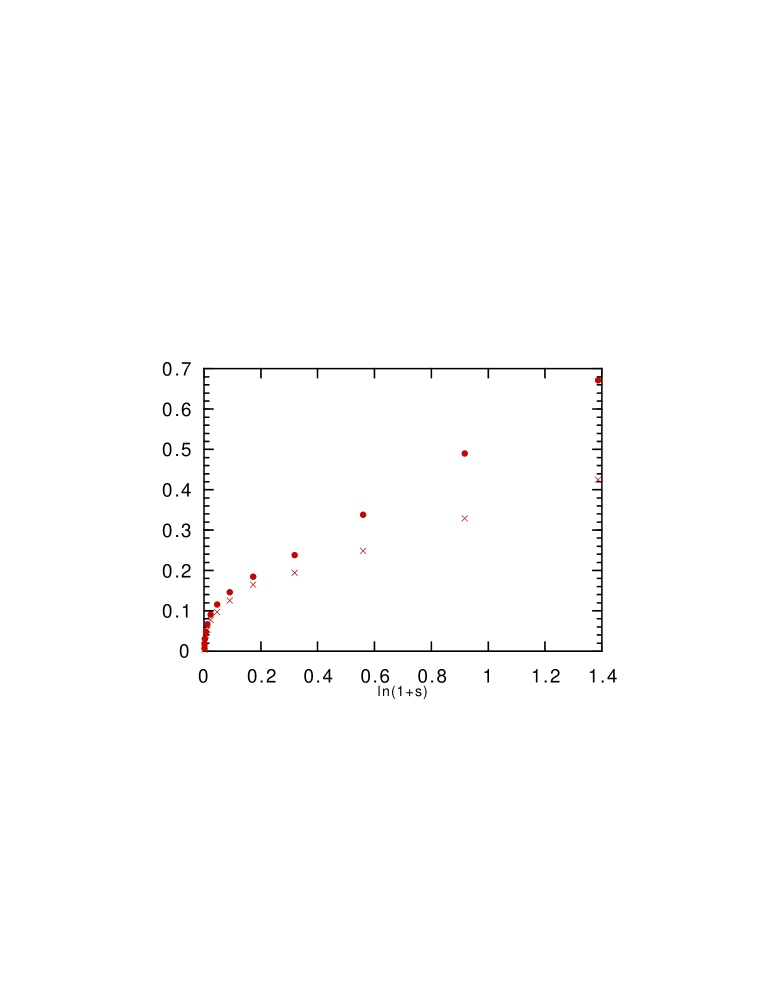
Figure 1: $\beta\Delta$ (points) and $R$ (crosses) as function the ratio $\ln(1+s)\equiv\ln(1+t/t_{w})$ at $\Gamma=1.7$ for $t_{w}=2048.$

The usual fluctuation theorem tells that at equilibrium $\beta\Delta=R$. This relation holds in spite of the fact that $\Delta(t,t_{w})$ is not the product of two observables one at time $t_{w}$, the other at time $t_{w}+t$. However it can be written as

$$\Delta(t,t_{w})\equiv{\sum_{i=1,N}{\bf x}_{i}(t_{w})^{2}+{\bf x}_{i}(t_{w}+t))^{2}-2{\bf x}_{i}(t_{w})\cdot{\bf x}_{i}(t_{w}+t))}/{N}$$ (14)

and a detailed analysis [17] shows that the fluctuation dissipation theorem is valid also in this case.

In the following we will look for the validity in the low temperature region of the generalized relation $\beta X(\Delta)\Delta=R$. This relation can be valid only in the region where the diffusion constant $D$ is equal to zero. Strictly speaking also in the glassy region $D\neq 0$, because diffusion may always happens by interchanging two nearby particles ($D$ is different from zero also in a crystal); however if the times are not too large the value of $D$ is so small in the glassy phase that this process may be neglected in a first approximation.

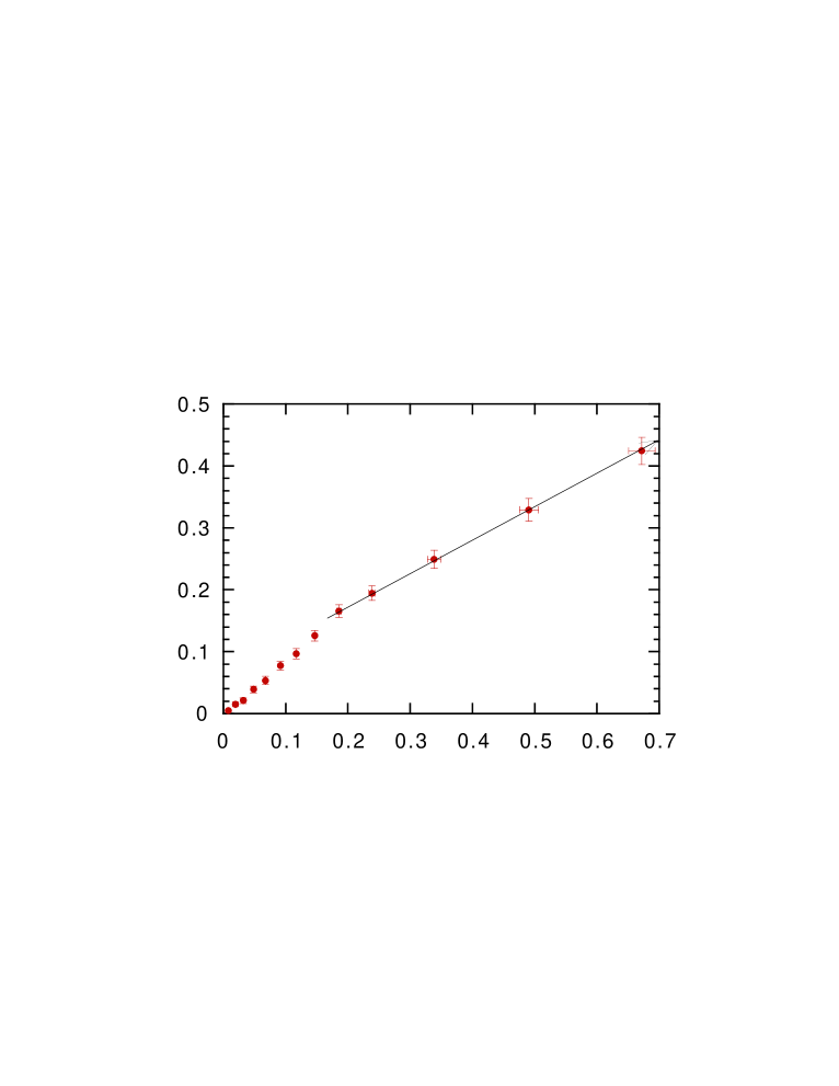
Figure 2: $R$ versus $\beta\Delta$ at $\Gamma=1.6$ for $t_{w}=t_{w}=8192.$ and $t_{w}=2048$

We have done simulations for $N=66$. For $N=66$ we average over 250 samples in absence of the force and on 1000 samples in presence of the force. We have done simulations for $\Gamma=1.4,1.5...2.0\$. The dynamics was implemented using the Monte Carlo method, with an acceptance rate fixed around .4. In order to decrease the error on the determination of $R$ we follow (as suggested in [18]) the method of computing in the same simulation the response function for different particles [19]. In other words we add to the Hamiltonian the term $\epsilon\sum_{k=1,N}{\bf}f_{k}\cdot{\bf x}_{k}$ where the $f$ are random Gaussian vectors of average squared length equal to 3. The quantity $R$ can be computed as the average over $f$ of

$${\sum_{k=1,N}{\bf f}_{k}\cdot{\bf x}_{k}(t_{w}+t))\over N\epsilon}.$$ (15)

The value of $\epsilon$ should be sufficient small in order to avoid non linear effects: we have done extensive tests for $\epsilon=.1$ and $\epsilon=.2$. We found that $\epsilon=.2$ is in the linear region, but we have followed the more conservative option $\epsilon=.1$. We present the results for $t_{w}=2048$. We have done also some simulations at $t_{w}=8192$, but we have not observed any systematic shift.

In fig.1 we show the dependence of $\Delta$ and $R$ on the ratio $s\equiv t/t_{w}$ in the low temperature region, i.e. at $\Gamma=1.7$ for $t_{w}=2048$. They coincide in the small $s$ region, where FDT holds, but they differ for $s>.1$.

In fig.2 we show $R$ versus $\beta\Delta$ at $t_{w}=2048$, still at $\Gamma=1.7$. We see two linear regions with different slope as follows from the assumption of one step replica symmetry breaking. The slope in the first region is 1, as expected form the FDT theorem, while tre slope in the second region is definitively smaller that 1.

Also the data at different temperatures for all values of $\Gamma\geq 1.5$ show a similar behaviour. The value of $R$ in the region where the FDT relation does not hold can be very well fitted by a linear function of $\Delta$ as can be seen in fig. 2.The region where a linear fit (with $m<1$) is quite good correspond to $t/t_{w}>.2$. The fitted value of $m\equiv\partial R/\partial(\beta\Delta)$ is displayed in fig. 3. When $m$ becomes equal to 1, the fluctuation dissipation theorem holds in the whole region and this happens at higher temperatures. The straight line is the prediction of the approximation $m(T)=T/T_{c}$, using $\Gamma_{c}=1.45$ which seems to be rather good..

The value of $m$ we find at $\Gamma=1.8$ (i.e. $m=.33\pm.04$) is compatible with the value $(m=.3\pm.1$) of ref. [6] extracted from the fluctuation of the stress energy tensor. The method described in this note is much more accurate for two reasons:

• The quantities which we consider becomes larger when we enter in the OFDR region: they increase (not decrease) as function of time.

• The correlation quantity we measure is an intensive quantity which becomes self averaging in the limit of infinite volume.

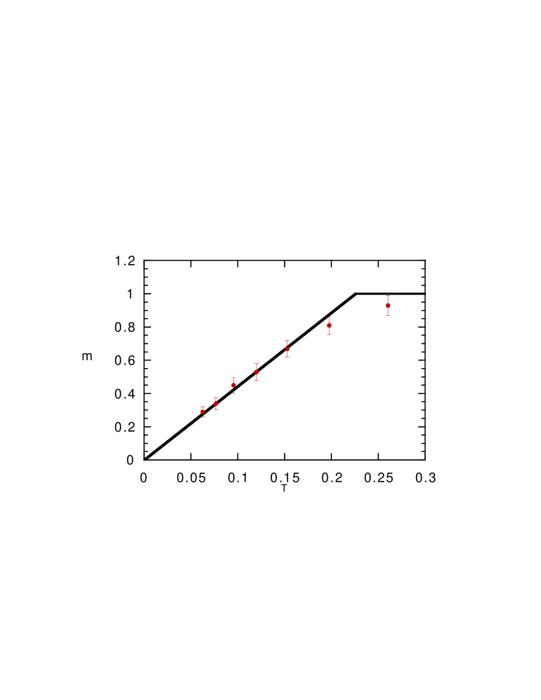
Figure 3: The quantity $m\equiv{\partial R\over\partial\beta\Delta}$ as $t_{w}=2048$ as function of the temperature. The straight line is the prediction of the approximation $m(T)=T/T_{c}$.

It is amusing to notice (as stressed to me by G. Ruocco) that the simple aging relation $\Delta(t_{w},t_{w})=cost$ for large $t_{w}$ implies that the particle move in average by a constant amount in each interval of time $2^{K}<t<2^{K+1}$. If we assume that the movement in each time interval are uncorrelated, it follows that in the glassy phase $\Delta(t,t_{w})\propto\ln(1+t/t_{w})$ for not too small $t/t_{w}$. This is what happens outside the FDT region, (i.e. $t/t_{w}>.2$), as it can be seen from fig. 1. In fig. 4 we show the data for $t_{w}=1$, i.e. the distance from the initial configuration. The data seem to display a very nice logarithmic behaviour.

All these results are in very good agreement with the theoretical expectations based on our knowledge extracted from the mean field theory for generalized spin glass models. The approximation $m(T)=T/T_{c}$ seems to work with an embarrassing precision. We can conclude that the ideas developed for generalized spin glasses have a much wider range of application than the models from which they have been extracted. It likely that they reflect quite general properties of the phase space and therefore they can be applied in cases which are quite different from the original ones.

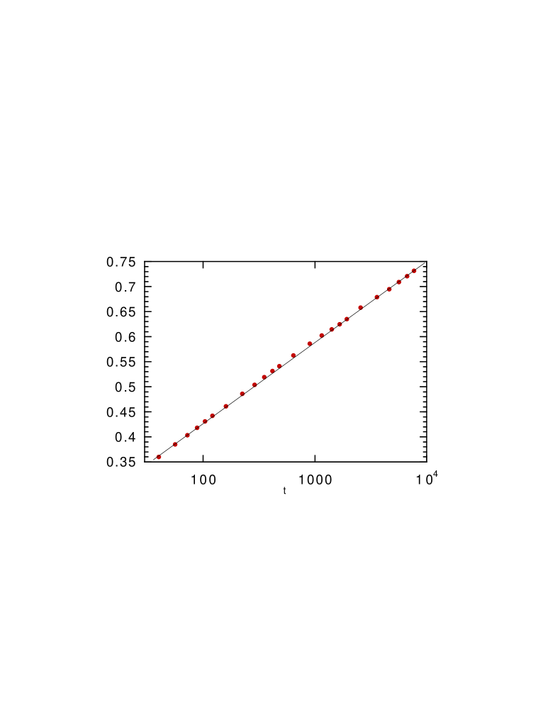
Figure 4: The distance from the initial configuration as function of the time in a logarithmic scale.

The most urgent theoretical task would be now to develop an analytic theory for glasses in the low temperature region from which one could compute the function $m(t)$. This goal should not be out of reach: a first step in this direction can be found in [20]

References

- [1]
- [2] L. F. Cugliandolo and J.Kurchan, Phys. Rev. Lett. 71, 1 (1993).
- [3] S. Franz and M. Mézard On mean-field glassy dynamics out of equilibrium, cond-mat 9403004.
- [4] J.-P. Bouchaud, L. Cugliandolo, J. Kurchan, Marc Mézard, cond-mat 9511042.
- [5] G. Parisi, Short time aging in binary glasses, cond-mat 9701015.
- [6] G. Parisi, Numerical indications for the existence of a thermodynamic transition in binary glasses, cond-mat 9701100.
- [7] J.-P. Bouchaud; J. Phys. France 2 1705, (1992).
- [8] L. C. E. Struik; Physical aging in amorphous polymers and other materials (Elsevier, Houston 1978).
- [9] M.Mézard, G.Parisi and M.A.Virasoro, Spin glass theory and beyond, World Scientific (Singapore 1987).
- [10] G.Parisi, Field Theory, Disorder and Simulations, World Scientific, (Singapore 1992).
- [11] S. Franz and H. Rieger Phys. J. Stat. Phys. 79 749 (1995).
- [12] E. Marinari, G. Parisi and F. Ritort, J. Phys. A: Math. Gen. 27 7615 (1994).
- [13] B.Bernu, J.-P. Hansen, Y. Hitawari and G. Pastore, Phys. Rev. A36 4891 (1987).
- [14] J.-L. Barrat, J-N. Roux and J.-P. Hansen, Chem. Phys. 149, 197 (1990).
- [15] J.-P. Hansen and S. Yip, Trans. Theory and Stat. Phys. 24, 1149 (1995).
- [16] D. Lancaster and G. Parisi, A Study of Activated Processes in Soft Sphere Glass, cond-mat 9701045.
- [17] L. Cugliandolo and J. Kurchan and G. Parisi, Off equilibrium dynamics and aging in unfrustrated systems, cond-mat/9406053, J. Phys. I (France) 4 1691 (1994).
- [18] L. Cugliandolo and J. Kurchan, private communication.
- [19] A. Billoire, E. Marinari, G. Parisi, Phys. Lett. 162B (1985) 160.
- [20] M.Mézard and G.Parisi, A tentative Replica Study of the Glass Transition, cond-mat/9602002.