Two interacting particles in a random potential:
The random matrix model revisited

Abstract

We reinvestigate the validity of mapping the problem of two onsite interacting particles in a random potential onto an effective random matrix model. To this end we first study numerically how the non-interacting basis is coupled by the interaction. Our results indicate that the typical coupling matrix element decreases significantly faster with increasing single-particle localization length than is assumed in the random matrix model. We further show that even for models where the dependency of the coupling matrix element on the single-particle localization length is correctly described by the corresponding random matrix model its predictions for the localization length can be qualitatively incorrect. These results indicate that the mapping of an interacting random system onto an effective random matrix model is potentially dangerous. We also discuss how Imry’s block-scaling picture for two interacting particles is influenced by the above arguments.

I Introduction

The interplay of disorder and many-body interactions in electronic systems has been studied intensively within the last two decades.[1] For non-interacting electrons, the highly successful “scaling hypothesis of localization” was put forward in 1979 by Abrahams et al.,[2] but the role played by many-particle interactions is much less understood and still no entirely consistent picture exists.[1] The recent discovery of a metal-insulator transition in certain two-dimensional electron gases at zero magnetic field [3] has renewed the interest in this problem, since in the samples considered the electron interaction is estimated to be much larger than the Fermi energy. [3] Thus the observed transition may be due to an interaction-driven enhancement of the conductivity.

The simplest version of the interacting disordered particle problem is perhaps the case of just two interacting particles (TIP) in a random potential in one dimension (1D). For a Hubbard on-site interaction this problem has recently also attracted a lot of attention after Shepelyansky [4, 5] argued that attractive as well as repulsive interactions between the two particles (bosons or fermions) lead to the formation of particle pairs whose localization length $\lambda_{2}$ is much larger than the single-particle (SP) localization length $\lambda_{1}$.[6] Based on a mapping of the TIP Hamiltonian onto an effective random matrix model (RMM) he predicted

$$\lambda_{2}\sim(U/V)^{2}\lambda_{1}^{2}$$ (1)

at two-particle energy $E=0$, with $V$ the nearest-neighbor transfer matrix element and $U$ the Hubbard interaction strength. Shortly afterwards, Imry [7] used a Thouless-type block-scaling picture (BSP) in support of this. The most surprising aspect of Eq. (1) is the fact that in the limit of weak disorder the ratio $\lambda_{2}/\lambda_{1}$ diverges. Thus, in the limit of weak disorder the particle pair can travel infinitely further than a SP. This should be contrasted with renormalization group studies of the 1D Hubbard model at finite particle density which indicate that a repulsive onsite interaction leads to a strongly localized ground state.[8]

Subsequent analytical investigations further explored the mapped TIP problem as an RMM problem.[9, 10, 11, 12] Direct numerical approaches to the TIP problem have been based on the time evolution of wave packets, [4] transfer matrix methods (TMM),[13] Green function approaches,[14, 15] or exact diagonalization [16]. In these investigations usually an enhancement of $\lambda_{2}$ compared to $\lambda_{1}$ has been found but the quantitative results differ both from the analytical prediction in Eq. (1), and from each other. Furthermore, a check of the functional dependence of $\lambda_{2}$ on $\lambda_{1}$ is numerically very expensive since it requires very large system sizes. Following the approach of Ref. [13], two of us studied the TIP problem by a different TMM [17] and found that (i) the enhancement $\lambda_{2}/\lambda_{1}$ decreases with increasing system size $M$, (ii) the behavior of $\lambda_{2}$ for $U=0$ is equal to $\lambda_{1}$ in the limit $M\rightarrow\infty$ only, and (iii) the enhancement $\lambda_{2}/\lambda_{1}$ also vanishes completely in this limit. Therefore it was concluded [17] that the TMM applied to the TIP problem in 1D measures an enhancement of the localization length which is entirely due to the finiteness of the systems considered.

In this paper we return the attention to the original mapping [4] of the TIP problem onto an effective RMM. We argue that the mapping as in Ref. [4] is potentially dangerous since (A) it overestimates the typical coupling matrix element and (B) it neglects phase correlations which we believe to be essential, because it is known that interference effects are responsible for Anderson localization to begin with. In order to establish that the mapping procedure [4] can lead to incorrect results we first numerically investigate the interaction-induced coupling matrix elements between the non-interacting basis states for various values of the SP localization length. We find that the typical coupling matrix element decreases significantly faster with increasing SP localization length than assumed in Ref. [4]. This alone would lead to a significantly smaller increase, if any, of the TIP localization length than in Eq. (1). We further show that even if the RMM correctly described the dependency of the coupling matrix element on the SP localization length, its results for the TIP localization length cannot be trusted. To this end we present two simple physical examples, namely Anderson models with additional perturbing random potentials for which the RMM mapping yields the same enhancement of the localization length as for the TIP problem. However, for our examples this enhancement is obviously incorrect. We also show that analogous problems exist for the BSP.[7] We argue that the failure of the RMM approach in our toy models is caused by neglecting the correlations between the coupling matrix elements. This has already been made responsible [13, 14] for quantitative differences between Eq. (1) and numerical results for the TIP problem. We show, however, that neglecting the correlations not only changes the quantitative predictions of the theory but can lead to qualitatively incorrect results.

The paper is organized as follows. In section II we briefly summarize the RMM approach to the TIP problem. In section III we present our numerical results for the TIP coupling matrix elements and their dependence on the SP localization length. The failure of the RMM approach to correctly predict the localization length of two toy models is discussed in section IV while section V shows the failure of the BSP for these toy models. We discuss the relevance of our results for the original TIP problem and conclude in section VI.

II The random matrix model approach

Let us start by recalling the basic steps of the RMM approach [4] to TIP in a random potential. The relevant energy scales are chosen such that the SP band width $4V$ is larger than the (uniform) spread of the disorder $W$ which in turn is supposed to be larger than the interaction strength $U$. The basic idea is to represent the TIP Hamiltonian in the eigenbasis of the non-interacting problem and then to replace the full Hamiltonian by a suitably chosen random matrix.

The (non-interacting) SP eigenstates are approximately described by

$$\psi_{n}(x)\sim{1\over\sqrt{\lambda}_{1}}\exp\left[-\frac{|x-x_{n}|}{\lambda_{1}}+i\theta_{n}(x)\right],$$ (2)

where $x_{n}$ is the localization center of the $n$th eigenstate and $\theta_{n}(x)$ is a phase which appears to be random but contains all the information about interferences necessary for Anderson localization. In the absence of interactions and neglecting symmetry considerations the two-particle eigenstates are just products of two SP eigenstates,

$$\psi_{nm}(x,y)\sim{1\over\lambda_{1}}\exp\left[-\frac{|x-x_{n}|}{\lambda_{1}}-\frac{|y-y_{m}|}{\lambda_{1}}+i\theta_{n}(x)+i\theta_{m}(y)\right],$$ (3)

where $x$ and $y$ are the coordinates of the first and second particle, respectively. Switching on the Hubbard interaction $U(x,y)=U\delta_{xy}$ between the two particles induces transitions between the eigenstates $\psi_{nm}$ of the non-interacting problem. To estimate the transition rates it is first noted that the matrix element $\langle\psi_{nm}|U|\psi_{n^{\prime}m^{\prime}}\rangle$ is exponentially small for $|x_{n}-y_{m}|>\lambda_{1}$ or $|x_{n^{\prime}}-y_{m^{\prime}}|>\lambda_{1}$ or $|x_{n}-x_{n^{\prime}}|>\lambda_{1}$ or $|y_{m}-y_{m^{\prime}}|>\lambda_{1}$. Thus, the interaction couples each of the two-particle states (3) close to the diagonal in the 2D configuration space ($|x_{n}-y_{m}|<\lambda_{1}$) to ${\cal O}(\lambda_{1}^{2})$ other such states. The interaction matrix element is then the sum of $\lambda_{1}$ contributions each with magnitude $U\lambda_{1}^{-2}$ and approximately random phases. Neglecting possible correlations among these contributions, Shepelyansky found the magnitude $u$ of the matrix element

$$u_{nmn^{\prime}m^{\prime}}=\langle\psi_{nm}|U|\psi_{n^{\prime}m^{\prime}}\rangle\sim U\lambda_{1}^{-3/2},$$ (4)

independent of the interaction being attractive, repulsive or even random. Eq. (4) is one of the essential ingredients of the RMM. In section III we will present numerical data in order to check its validity. We remark that the validity of Eq. (4) has recently been questioned in Ref. [18] where the authors have computed a different estimate taking into account the nearly Bloch-like structure of the eigenstates for small $W$.

Shepelyansky [4, 5] now replaced the full TIP Hamiltonian by an effective RMM for those of the two-particle states that are coupled by the interaction. Thus the Hamiltonian matrix becomes a banded matrix whose elements are independent Gaussian random numbers with zero mean. The diagonal elements are drawn from a distribution of width $V$, because for small disorder $W$ the nearest-neighbor transfer $V$ determines the band width of the SP states. The distribution of the off-diagonal elements has width $|U|\lambda_{1}^{-3/2}$ within a band of width $\lambda_{1}$.

In order to obtain results for the localization properties of such an RMM one has to distinguish different regimes, depending on the strength of the interaction. If the interaction is strong enough to couple many non-interacting eigenstates, i.e., the inverse lifetime $\Gamma$ of a non-interacting state is large compared to the level spacing of the coupled states, Fermi’s golden rule can be applied. This regime was investigated in Ref. [4] and also gives the largest enhancement of $\lambda_{2}$ compared to $\lambda_{1}$. We note that in this regime the level-spacing distribution of the non-interacting system cannot play a significant role since the interactions couple a large number of levels and lead to a decay into a quasi-continuum of final states. In the opposite limit, i.e., if the interaction couples only few non-interacting eigenstates, Fermi’s golden rule cannot be applied. Instead, one finds Rabi oscillations between the few coupled states.[10] We note that in this regime the level spacing distribution of the non-interacting states becomes important. In the following we will only consider the golden rule regime.

The localization length of the effective RMM can be determined by several equivalent methods. Here we follow Shepelyansky:[5] Calculating the decay rate $\Gamma$ of a non-interacting eigenstate by means of Fermi’s golden rule gives $\Gamma\sim U^{2}/\lambda_{1}V$. Since the typical hopping distance is of the order of $\lambda_{1}$ the diffusion constant is $D\sim U^{2}\lambda_{1}/V$. Within a time $\tau$ the particle pair visits $N\sim U\lambda_{1}^{3/2}V^{-1/2}\tau^{1/2}$ states. Diffusion stops when the level spacing of the visited states is of the order of the frequency resolution $1/\tau$. This determines the cut-off time $\tau^{*}$ and the corresponding pair-localization length is obtained as $\lambda_{2}\sim\sqrt{D\tau^{*}}\sim(U/V)^{2}\lambda_{1}^{2}$ in agreement with Eq. (1). Applicability of Fermi’s golden rule requires $\Gamma\gg V/\lambda_{1}^{2}$ which is equivalent to $U^{2}\lambda_{1}/V^{2}\gg 1$. This is exactly the condition for an enhancement of $\lambda_{2}$ compared to $\lambda_{1}$.

Let us recapitulate: The mapping of the TIP problem onto the RMM described above relies on two assumptions: (A) the non-interacting wavefunctions can be described by a decaying amplitude with finite localization length and a random phase which leads to the $U/\lambda_{1}^{3/2}$ behavior in Eq. (4) and (B) any correlations between the matrix elements in the Hamiltonian can be neglected. In the next two sections we will closer analyze the validity of these two assumptions.

III Numerical results for the matrix elements

In this section we present results for the interaction-induced coupling matrix elements in order to check whether they follow the $\lambda_{1}^{-3/2}$ power law (4) as assumed in Ref. [4]. Since $\lambda_{1}$ deviates from the simple power-law prediction [6] $\lambda_{1}\approx 104/W^{2}$ at $E=0$ already for $\lambda_{1}\lesssim 4$ ($W\gtrsim 5$), we have first computed $\lambda_{1}$ by TMM [6] in 1D with $0.1\%$ accuracy for all $W\geq 0.3$ ($\lambda_{1}\approx 1156$). We next exactly diagonalize the SP Hamiltonian and obtain the eigenstates. We then compute the “center-of-mass” (CM) of these eigenstates as $x_{n}=\sum_{x}x|\psi_{n}(x)|/\sum_{x}|\psi_{n}(x)|$. For hard wall boundary conditions, we have checked that using this definition of the CM we can reproduce the disorder dependence of $\lambda_{1}$ from the decay of the SP wave function $\psi_{n}$ via $1/\lambda_{1}=-\lim_{|x-x_{n}|\rightarrow\infty}\ln|\psi_{n}(x)|/|x-x_{n}|$ to within $10\%$ up to $\lambda_{1}=104$ ($W=1$) for $50$ samples of length $M=1200$. For periodic boundary conditions, we use a suitably generalized definition for the CM. We next calculate the matrix elements $\langle\psi_{nm}|U|\psi_{n^{\prime}m^{\prime}}\rangle$ for all states with appropriate CM, i.e., $|x_{n}-y_{m}|\leq\lambda_{1}$, $|x_{n^{\prime}}-y_{m^{\prime}}|\leq\lambda_{1}$, $|x_{n}-x_{n^{\prime}}|\leq\lambda_{1}$ and $|y_{m}-y_{m^{\prime}}|\leq\lambda_{1}$. Since the interaction strength $U$ appears only as a multiplicative prefactor in the matrix elements, we choose $U=1$ in all of what follows. We emphasize that the bottleneck in such a computation is not the system size $M$, but rather the exponentially growing number of overlapping matrix elements for increasing $\lambda_{1}$.

In Fig. 1 we show the unnormalized probability distributions $P_{\text{d/o}}(u)$ of diagonal and off-diagonal coupling matrix elements. $P_{\text{d/o}}(u)$ was computed at disorder $W=2$ where the enhancement of $\lambda_{2}$ with respect to $\lambda_{1}$ is expected to be large.[13, 14, 15] We have averaged over $50$ different disorder configurations for $M=200$. For a more detailed inspection we plot the data on a doubly logarithmic scale in Figs. 2 and 3. As already discussed before [13, 14, 19] we note that (i) the diagonal elements are non-negative, (ii) $P_{\text{o}}(u)$ is symmetric around $u=0$. The deviation from symmetry for $|u|\gtrsim 0.02$, i.e., $P_{\text{o}}(|u|)>P_{\text{o}}(-|u|)$, is most likely due to the finite size of the samples. More importantly, (iii) $P_{\text{o}}(u)$ is strongly non-Gaussian. We remark that a fit to a Lorentzian distribution does also not describe the data. (iv) apart from a peak at $u\approx 0$, $P_{\text{d}}(u)$ is approximately Gaussian, (v) $P_{\text{o}}(u)$ and $P_{\text{d}}(u)$ have rather long tails, (vi) the total distribution of matrix elements $P(u)$ is dominated by $P_{\text{o}}(u)$ (as in any matrix) and thus $P(u)$ is strongly non-Gaussian with long tails.

For such a non-Gaussian $P(u)$ the average of the absolute matrix elements $u_{\text{abs}}=\langle|u|\rangle$, with $\langle\cdot\rangle$ denoting the average over $u$ according to $P(u)$, is strongly influenced by rare events in the tails of the distribution. This is even more so when using the mean-square value $\sqrt{\langle u^{2}\rangle}$. However, in the physical problem considered here these rare large couplings lead to oscillations of the system between the corresponding two TIP states but not to delocalization. The typical value $u_{\text{typ}}$ is thus better defined as the logarithmic average $u_{\text{typ}}=\exp[\langle\log(|u|)\rangle]$.

We have calculated both $u_{\text{abs}}$ and $u_{\text{typ}}$ for different values of $W$ and $50$ samples for $M\leq 200$ and $30$ samples for $M=250$. As shown in Fig. 4, the dependence of $u_{\text{abs}}$ on $\lambda_{1}$ for $\lambda_{1}>5$ follows $u_{\text{abs}}\propto\lambda_{1}^{-\alpha}$. A fit for $20\leq\lambda_{1}\leq 111$ yields $\alpha={-1.5\pm 0.1}$ as predicted in Ref. [4]. However, the typical TIP matrix element $u_{\text{typ}}$ decreases much faster with increasing $\lambda_{1}$. Fitting the $u_{\text{typ}}$ data to a power law for $20\leq\lambda_{1}\leq 111$, we obtain $\alpha=1.95\pm 0.10$. Furthermore, for the largest $\lambda_{1}$ the numerical data deviate — albeit weakly — from the above power law showing a slight downward curvature in the double-logarithmic representation. In fact, if we only consider the data points from the large chains with $M=250$, we already find $\alpha=2.02\pm 0.10$. This indicates that asymptotically the dependence is even stronger than $\lambda_{1}^{-1.95}$.

In Fig. 5, we show $u_{\text{abs}}$ and $u_{\text{typ}}$ for the diagonal matrix elements only. For $20\leq\lambda_{1}\leq 111$ the data can be fitted by $u_{\text{d,abs}}\propto\lambda_{1}^{-0.9\pm 0.1}$ and $u_{\text{d,typ}}\propto\lambda_{1}^{-1.0\pm 0.1}$. Thus as expected $u_{\text{d,abs}}$ and $u_{\text{d,typ}}$ behave similarly since $P_{\text{d}}(u)$ may be approximated by a Gaussian distribution. Furthermore, $\alpha=1$ is in agreement with Eq. (21) of Ref. [18].

Repeating the RMM calculation of section II with a dependence $u_{\text{typ}}\sim U\lambda_{1}^{-\alpha}$ instead of Eq. (4), we obtain

$$\lambda_{2}\sim(U/V)^{2}\lambda_{1}^{-2\alpha+5}~{}.$$ (5)

If we use now use $\alpha=1.95\pm 0.10$ we find $\lambda_{2}\sim\lambda_{1}^{1.1\pm 0.2}$. However, as discussed above the true asymptotic dependence of $u_{\text{typ}}$ on $\lambda_{1}$ is likely to be even stronger than $\lambda_{1}^{-1.95}$ which in turn results in an even weaker enhancement of $\lambda_{2}$. We emphasize that the enhancement predicted by Shepelyansky [4, 5] will vanish for $\alpha=2$ in the limit $\lambda_{1}\to\infty$. A value of $\alpha>2$ will in fact correspond to even stronger localization of the TIP.

In order to further explore the validity of assumption (A) we compute $P_{\text{d/o}}(u)$ for a site-dependent random onsite interaction $U(x)\in[-U,+U]$, averaging as before over $50$ samples. If assumption (A) is correct, the resulting distribution of the coupling matrix elements should qualitatively be similar to the one obtained for the original TIP problem. But as shown in Figs. 2 and 3, we find that the randomness of the interaction already leads to a significant decrease of the long-range nature of $P(u)$. E.g., at $|u|=0.02$, there is a reduction in $P_{\text{d/o}}(0.02)$ by a factor of approximately $10$ for diagonal and approximately $5$ for off-diagonal matrix elements when compared to $P_{\text{d/o}}(0.02)$ of the original TIP problem. We further compute $P(u)$ for states with the same CM as previously, but otherwise chosen according to Eq. (3) with uncorrelated random phases and exponentially decaying envelope. The disorder averaging is again over $50$ samples. As shown in Fig. 1, $P_{\text{d}}(u)$ now has a maximum at finite $u$. For these states $P_{\text{o}}(u)$ is well approximated by a Gaussian just as expected by Shepelyansky.[4, 5] The double-logarithmic plot of Fig. 3 shows deviations from the symmetry $P_{\text{o}}(u)=P_{\text{o}}(-u)$ for $|u|\gtrsim 0.008$, i.e., $P_{\text{o}}(|u|)>P_{\text{o}}(-|u|)$. As for the TIP problem, we attribute this to the finite size of the samples considered. Again, we note that when compared to $P_{\text{o}}(u)$ for the TIP problem, the present distribution of matrix elements decreases much faster and at $|u|=0.02$ is about one order of magnitude smaller. Furthermore, for $|u|>0.008$ the distribution $P_{\text{o}}(u)$ is also smaller than that for the model with random interaction. Thus assumption (A) clearly oversimplifies the problem and the neglect of phase correlations leads to a wrong $P_{\text{d/o}}(u)$. In Fig. 4, we show $u_{\text{abs}}$ and $u_{\text{typ}}$ for the artificial states of Eq. (3). In complete agreement with our previous discussion, we find that for $\lambda_{1}>20$ both the average and the typical matrix element vary as $u\propto\lambda_{1}^{-1.4\pm 0.1}$ compatible with $\alpha=3/2$.

In Fig. 4, we show also TIP data for chain lengths $M=100$. We note that deviations due to the small system size lead to a smaller slope for $u_{\text{abs}}$ and thus may give rise to an apparent enhancement of $\alpha$. As can be seen in the figure, this decreasing of the slope happens for $M=100$ already at $\lambda_{1}\gtrsim 20$ ($W\lesssim 2.3$). A power-law fit for $30\leq\lambda_{1}\leq 57$ yields $u_{\text{abs}}\propto\lambda_{1}^{-1.39\pm 0.10}$. The finite-size deviations for $u_{\text{typ}}$ are different. A power-law fit for $7\leq\lambda_{1}\leq 30$ gives $u_{\text{typ}}\propto\lambda_{1}^{-1.77\pm 0.10}$ whereas for $30\leq\lambda_{1}\leq 57$ we find $u_{\text{typ}}\propto\lambda_{1}^{-2.06\pm 0.10}$. Thus first there is a decrease of $\alpha$ followed by a finite-size increase of $\alpha$. For still larger $\lambda_{1}\gg M/2$ the finite-size deviations of $u_{\text{abs}}$ and $u_{\text{typ}}$ become very large even resulting in a positive slope. This finite-size effect may be at least partially responsible for the enhancement observed in Refs. [13] and [17] for this value of $M$.

In Fig. 6, we show $u_{\text{abs}}$ and $u_{\text{typ}}$ for $M=100$ with hard wall and periodic boundary conditions. Up to $\lambda_{1}\approx 10$, the data for both boundary conditions agree quite well. For $10\leq\lambda_{1}\leq 25$, the slope for the data with periodic boundaries is slightly smaller than for the data with hard wall boundaries. Lastly, around $\lambda_{1}\approx M/2$, the data for periodic boundaries shows a very fast decrease of $u$. Thus the data for periodic boundaries is influenced by the finite size of the sample already earlier than the data for hard wall boundaries. Nevertheless, except for these finite size effects, our results for both boundary conditions are similar and we will restrict ourselves to the hard wall boundaries in the following. We remark that most numerical studies of the TIP problem also use this type of boundaries. [13, 14, 15, 16, 17]

IV Failure of the RMM approach for toy models

In this section we show that even an RMM which contains the correct dependence of the coupling matrix elements on the SP localization length may give qualitatively incorrect results. To this end we consider two toy models, viz. Anderson models of localization with additional perturbing random potentials. By a procedure analogous to that of section II we map these models onto RMMs and then show that these RMMs give erroneous enhancements of the localization length.

A 2D Anderson model with perturbation on a line

The first example is set up to lead to the same RMM as the TIP problem. It consists of the usual 2D Anderson model of localization perturbed by an additional weak random potential of strength $U$ at the diagonal $x=y$ in real space. Since this increases the width of the disorder distribution at the diagonal we expect the localization length to decrease. We now map onto an RMM as in Refs. [4, 5]. As above, the eigenstates of the unperturbed system are localized with a localization length $\lambda_{1}$ and approximately given by

$$\psi_{n}(x,y)\sim{1\over\lambda_{1}}\exp\left[-\frac{|{\bf r}-{\bf r}_{n}|}{\lambda_{1}}+i\theta_{n}({\bf r})\right]$$ (6)

where ${\bf r}=(x,y)^{T}$ is the coordinate vector of the particle and $\theta$ is again a phase which is assumed to be random. The Hamiltonian of this model differs from the TIP Hamiltonian in two points: (i) the diagonal elements are independent random numbers instead of being partially correlated as in the TIP problem and (ii) the interaction potential $U(x,x)\in[-U,U]$ at each site of the diagonal is random instead of having a definite sign and modulus $U$ as in the TIP problem. However, none of these points enters the mapping procedure outlined above. Thus, applying exactly the same arguments as for the TIP problem in section II we find that the perturbation couples each state close to the diagonal ($|x_{n}-y_{n}|<\lambda_{1}$) to ${\cal O}(\lambda_{1}^{2})$ other such states. The interaction matrix element is again a sum of ${\cal O}(\lambda_{1})$ terms of magnitude $U/\lambda_{1}^{2}$ and random phases giving a typical value of $U\lambda_{1}^{-3/2}$. Consequently, our toy model is mapped onto exactly the same RMM as TIP in a random potential.

As for the TIP case we now numerically check the relation between the coupling matrix element and the SP localization length $\lambda_{1}$. We first note that the disorder dependence of $\lambda_{1}$ in the 2D Anderson model is no longer approximated by the simple power law cited in section III.[20] In fact, $\lambda_{1}$ is usually much larger in the 2D case for the same value of $W$. Thus we compute estimates $\lambda_{1}(M)$ as a function of $W$ for quasi-1D strips of finite strip width $M$ with $1\%$ accuracy by TMM. We remark that due to the self-averaging [20] of $1/\lambda_{1}(M)$ this is equivalent to computing $\lambda_{1}(M)$ for many samples of $M\times M$ disordered squares. In Fig. 7, we show data of $\lambda_{1}(M)$ as a function of $W$. We take $\lambda_{1}(50)$ to compute the coupling matrix elements. Since $\lambda_{1}(50)$ is always larger than for smaller system size, this choice only means that we sum over a few additional but very small terms when computing $u$. Next, we calculate both $u_{\text{abs}}$ and $u_{\text{typ}}$ for different values of $W$ and various $M\times M$ squares. Disorder averaging is over $20$ samples and we study $u_{\text{abs}}$ and $u_{\text{typ}}$ as functions of $\lambda_{1}(M)$. We emphasize that instead of the well-known extrapolations of $\lambda_{1}(M)$ to infinite system size by means of finite-size scaling,[20] we take the finite-size approximants $\lambda_{1}(M)$ on purpose, since we compute $\lambda_{2}$ also for comparable finite sizes only.

In Fig. 8 we show the computed distributions $P_{\text{d/o}}(u)$ for the present model. As for the TIP model the diagonal elements are non-negative and $P_{\text{d}}(u)$ has a large peak at $u=0$; $P_{\text{o}}(u)$ is again strongly non-Gaussian. The results for $u_{\text{abs}}$ and $u_{\text{typ}}$ are presented in Fig. 9. The dependence of $u_{\text{abs}}$ on $\lambda_{1}(M)$ for $2\leq\lambda_{1}(M)\leq 12$ follows $u_{\text{abs}}\propto\lambda_{1}(M)^{-1.6\pm 0.1}$ in agreement with our above prediction. Furthermore, here we also have $u_{\text{typ}}\propto\lambda_{1}(M)^{-1.5\pm 0.1}$. As before, we note that the slopes of $u_{\text{abs}}$ and $u_{\text{typ}}$ become smaller for $\lambda_{1}(M)\approx M/2$ due to the finite sample sizes. This finite-size effect is just the same as for TIP and thus further supports our use of the finite-size values $\lambda_{1}(M)$. We remark that if instead of $\lambda_{1}(M)$, we use $\lambda_{1}(50)$ for plotting the $u_{\text{abs}}$ and $u_{\text{typ}}$ data, that is irrespective of the system sizes for which they had been computed, we obtain $u_{\text{abs}}\propto\lambda_{1}^{-1.54\pm 0.10}$ and $u_{\text{typ}}\propto\lambda_{1}^{-1.47\pm 0.10}$. Thus both choices of $\lambda_{1}$ show that $u_{\text{abs}}$ and $u_{\text{typ}}$ vary as $\lambda_{1}^{-1.5}$ within the accuracy of the calculation.

Since our toy model is mapped onto the same RMM as the TIP problem the resulting localization length along the diagonal is also given by Eq. (1). We thus arrive at the surprising conclusion, that adding a weak random potential at the diagonal of a 2D Anderson model leads to an enormous enhancement of the localization length along this diagonal, in contradiction to the expectation expressed above, viz. that increasing disorder leads to stronger localization.

B 1D Anderson model with perturbation

An even more striking contradiction can be obtained for a 1D Anderson model of localization. The eigenstates are again given by Eq. (2) with $\lambda_{1}$ known from second order perturbation theory [21] and numerical calculations [6] to vary as $\lambda_{1}\sim V^{2}/W^{2}$ for small disorder. We now add a weak random potential of strength $U$ at all sites. Since the result is obviously a 1D Anderson model with a slightly higher disorder strength the localization length will be reduced, $\lambda_{1}(U)\sim V^{2}/(W^{2}+U^{2})$. Now we map onto an RMM according to Refs. [4, 5]. The additional potential leads to transitions between the unperturbed eigenstates $\psi_{n}$. Each such state is now coupled to ${\cal O}(\lambda_{1})$ other states by coupling matrix elements $\langle\psi_{n}|U|\psi_{n^{\prime}}\rangle$ with magnitude $u\sim U\lambda_{1}^{-1/2}$ since we sum over $\lambda_{1}$ contributions with magnitude $U/\lambda_{1}$ and supposedly random phases.

Again we numerically check the relation between $u_{\text{abs}}$ and $u_{\text{typ}}$ as functions of $\lambda_{1}$. In Fig. 10, we show results obtained for chains with various lengths and $50$ disorder configurations for each $W$. $\lambda_{1}$ is computed by TMM as in section III. In Fig. 11 we show the distributions $P_{\text{d/o}}(u)$. We note that $P_{\text{o}}(u)$ is non-Gaussian as for the TIP model and the perturbed 2D Anderson model. $P_{\text{d}}(u)$ is similar to the previous models, but the fluctuations are much larger. For $10\leq\lambda_{1}\leq 250$, $u_{\text{abs}}$ varies as $\lambda_{1}^{-0.48\pm 0.10}$ as we predicted above. $u_{\text{typ}}$ varies as $\lambda_{1}^{-0.59\pm 0.10}$. Both variations are compatible with $\alpha=1/2$. Again we need at least $\lambda_{1}\gtrsim M/2$ in order to suppress the effects of the finite chain lengths.

In analogy to section II the application of Fermi’s golden rule in this 1D case leads to a diffusion constant $D\sim U^{2}\lambda_{1}^{2}/V$. The number of states visited within a time $\tau$ is now $N\sim U\lambda_{1}V^{-1/2}\tau^{1/2}$. Again, diffusion stops at a time $\tau^{*}$ when the level spacing of the states visited equals the frequency resolution. This gives $\tau^{*}\sim U^{2}\lambda_{1}^{2}/V^{3}$. The localization length $\lambda$ of the perturbed system thus reads $\lambda\sim\sqrt{D\tau^{*}}\sim U^{2}\lambda_{1}^{2}$ as in Eq. (1), in clear contradiction to the correct result.

V Failure of the BSP for toy models

We now discuss the relation of our results to Imry’s BSP [7] for the TIP problem. In this approach one considers blocks of linear size $\lambda_{1}$ and calculates the dimensionless pair conductance on that scale,

$$g_{2}\sim{u^{2}\over\Delta^{2}},$$ (7)

where $u$ represents the typical interaction-induced coupling matrix element between states in neighboring blocks and $\Delta\sim V/\lambda_{1}^{2}$ is the level spacing within the block. If the typical coupling matrix element depends on $\lambda_{1}$ as $u\sim U\lambda_{1}^{-\alpha}$ the pair conductance obeys

$$g_{2}\sim(U/V)^{2}\lambda_{1}^{4-2\alpha}.$$ (8)

Again, an estimate analogous to Shepelyansky’s (4) gives $\alpha=3/2$ which leads to a strong enhancement of the pair conductance $g_{2}\sim\lambda_{1}$ as compared to the SP conductance $g_{1}$ which is of order unity on scale $\lambda_{1}$. In contrast, the numerical data of section III suggest that the pair conductance increases much less, viz. $g_{2}\sim(U/V)^{2}\lambda_{1}^{0.1\pm 0.2}$ for the fitted exponent $\alpha=1.95\pm 0.10$. Asymptotically for large $\lambda_{1}$ the pair conductance is likely to be enhanced even less than that. The behavior will be close to or even smaller than the marginal case $g_{2}\sim g_{1}$. All this is in complete agreement with our corresponding considerations for the RMM.

For the 2D Anderson model considered in the last section, the BSP can be applied analoguously. Again, we consider blocks of linear size $\lambda_{1}$ and compute the typical perturbation-induced matrix elements between these blocks as in section IV A. We then find that according to the BSP the conductance of a 2D Anderson model with additional weak perturbing potential along the diagonal is given by Eq. (7). Using $\alpha=1.5\pm 0.1$ as obtained in section IV A from the numerical data for $u_{\text{abs}}$ and $u_{\text{typ}}$, we then have $g_{2}\sim(U/V)^{2}\lambda_{1}$. Thus the BSP yields the same unphysical result as the RMM approach of section IV A.

Let us also apply the BSP to the 1D toy example. The level spacing in a 1D block of size $\lambda_{1}$ is $\Delta\sim V/\lambda_{1}$, and the coupling matrix element between states in neighboring blocks is $t\sim U\lambda_{1}^{-1/2}$. Thus, the conductance of the perturbed system on a scale $\lambda_{1}$ is obtained as $g_{p}\sim(U/V)^{2}\lambda_{1}$. For large $\lambda_{1}$ this again contradicts the correct result, viz. a decrease of the conductance compared to the unperturbed system.

Thus, the BSP applied to the two toy models introduced in section IV gives the same qualitatively incorrect results for the localization properties as the RMM. This is not surprising since the only ingredients of the BSP are the intra-block level spacing $\Delta\sim V/\lambda_{1}^{2}$ and the inter-block coupling matrix elements $u$ which also enter the RMM and have been discussed in section IV.

VI Conclusions

To summarize, we have reinvestigated the RMM approach to the problem of TIP in a random potential. We have shown that this kind of mapping an interacting disordered system onto an effective random matrix model is potentially dangerous since (A) it may overestimate the typical coupling matrix element and (B) it neglects correlations between the matrix elements.

In the first part of the paper we investigated the dependence of the matrix elements entering the RMM on the SP localization length $\lambda_{1}$. We found the dependence of the typical matrix element $u_{\text{typ}}$ to be significantly stronger than for the averaged absolute value $u_{\text{abs}}$ which is used in Refs. [4, 5, 7, 10, 12]. If the RMM approach of section II is modified by using the numerically determined relation between $u_{\text{typ}}$ and $\lambda_{1}$ instead of Eq. (4) the resulting enhancement of $\lambda_{2}$ with respect to $\lambda_{1}$ becomes much weaker. We showed that the difference between $u_{\text{typ}}$ and $u_{\text{abs}}$ is due to the over-simplified assumption (A) that the wave functions behave according to Eq. (2). Moreover, our data for $u_{\text{typ}}$ show systematic deviations from power-law behavior indicating that the true asymptotic dependence of $u_{\text{typ}}$ on $\lambda_{1}$ is likely to be very close to or stronger than the marginal case $u_{\text{typ}}\sim\lambda_{1}^{-2}$. If the asymptotic dependence is stronger than $u_{\text{typ}}\sim\lambda_{1}^{-2}$ the Shepelyansky enhancement vanishes in the limit of large $\lambda_{1}$ even within the RMM approach.

In the second part of this paper we showed that there are physical situations where mapping onto an RMM as in Ref. [4] gives qualitatively incorrect results, e.g., an increase of the localization length in physical situations where it should rather decrease. This failure occurs even if the RMM contains the correct dependence of $u_{\text{typ}}$ on $\lambda_{1}$. This shows in contrast to assumption (B) that in general the correlations between the matrix elements cannot be neglected since they contain information essential for the interference leading to Anderson localization. Note that the approach of Ref. [18], while correcting assumption (A), still includes a mapping onto an RMM and thus is plagued by the same problems as assumption (B). Analogously, in Ref. [22] the decay rate $\Gamma$ is calculated numerically, avoiding assumption (A). However, the formula $\lambda_{2}/\lambda_{1}\sim\Gamma\lambda_{1}^{2}/V$ employed in Ref. [22] is also based on an assumption similar to (B).

Let us comment on the relevance of this work for the original problem of TIP in a random potential. None of our results constitute, of course, a proof that the enhancement of the TIP localization length $\lambda_{2}$ predicted in Ref. [4] does not exist. However, in our opinion, the toy counter examples to the RMM approach introduced in section IV let the analytical arguments giving Eq. (1) appear much weaker. Taking the RMM approach seriously but using the numerical results for the typical coupling matrix element presented in section III we find that the dependence of the enhancement factor $\lambda_{2}/\lambda_{1}$ on $\lambda_{1}$ is significantly weaker than in Eq. (1). Nevertheless, an enhancement of the pair localization length for TIP as compared to $\lambda_{1}$ may still exist, although the underlying mechanism should then be different. Results supporting such an enhancement have been obtained by Green function methods [14] together with finite-size scaling arguments.[15] The most recent data obtained in Ref. [15] finds an exponent $\alpha=1.45\pm 0.2$ for $U=1$.

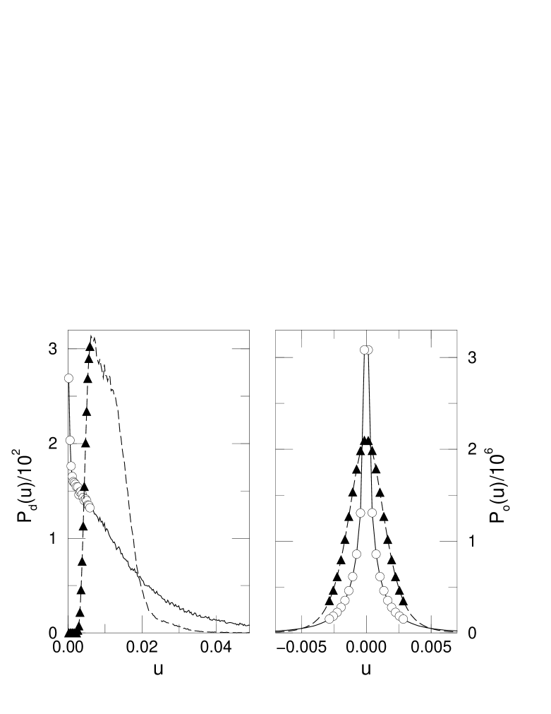
FIG. 1.: Unnormalized distribution $P_{\text{d/o}}(u)$ of the diagonal (left panel) and off-diagonal (right panel) coupling matrix elements $u$ with bin width $\Delta=0.0003$ for $\lambda_{1}=26$ ($W=2$) and $M=200$. Circles and solid lines indicate TIP data, triangles and dashed lines indicate matrix elements computed using Eq. (3). The symbols mark the data for the 20 smallest $|u|$.

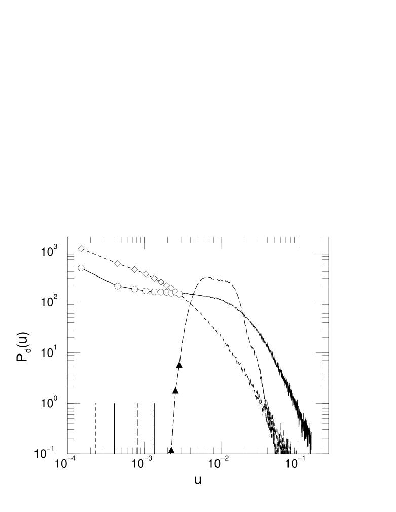
FIG. 2.: Double-logarithmic plot of the unnormalized distribution $P_{\text{d}}(u)$ of the diagonal coupling matrix elements $u$ for $\lambda_{1}=26$ ($W=2$) and $M=200$ as in Fig. 1. Solid, short-dashed, and long-dashed lines correspond to the TIP problem, the TIP problem with random interaction, and Eq. (3), respectively. Circles, diamonds and triangles mark the data for the $10$ smallest $u$ in each case, only three of which are larger than $10^{-1}$ for the triangles. The vertical lines on the $u$-axis indicate $u_{\text{abs}}$ (right) and $u_{\text{typ}}$ (left) as computed from the total distribution $P(u)$.

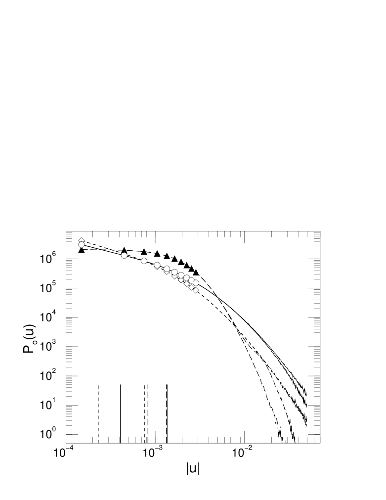
FIG. 3.: Double-logarithmic plot of the unnormalized distribution $P_{\text{o}}(u)$ of the off-diagonal coupling matrix elements $u$ for $\lambda_{1}=26$ ($W=2$) and $M=200$ as in Fig. 1. Solid, short-dashed, and long-dashed lines correspond to the TIP problem, the TIP problem with random interaction, and Eq. (3), respectively. Circles, diamonds and triangles mark the data for the $10$ smallest $|u|$ in each case. The vertical lines on the $u$-axis indicate $u_{\text{abs}}$ (right) and $u_{\text{typ}}$ (left) as computed from the total distribution $P(u)$.

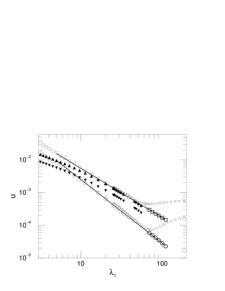
FIG. 4.: Dependence of $u_{\text{abs}}$ ($\Box$, $\blacktriangle$) and $u_{\text{typ}}$ ($\circ$, $\blacktriangledown$) on $\lambda_{1}$ for the TIP eigenstates (open symbols) and states chosen according to Eq. (3) (filled symbols) for $M=200$. The small (bold) symbols indicate $u_{\text{abs}}$ and $u_{\text{typ}}$ for $M=100$ ($M=250$). The solid lines represent the power laws $u_{\text{abs}}\sim\lambda_{1}^{-1.5}$ and $u_{\text{typ}}\sim\lambda_{1}^{-1.95}$.

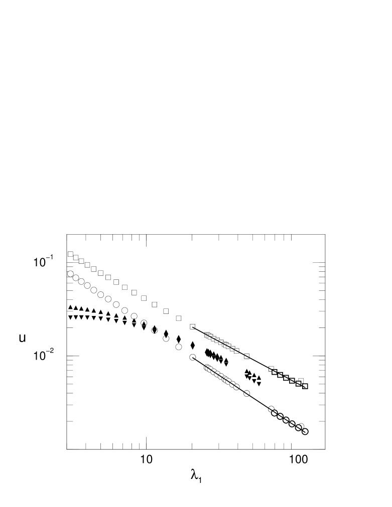
FIG. 5.: Dependence of $u_{\text{d,abs}}$ ($\Box$, $\blacktriangle$) and $u_{\text{d,typ}}$ ($\circ$, $\blacktriangledown$), i.e., for diagonal matrix elements only, on $\lambda_{1}$ for the TIP eigenstates (open symbols) and states chosen according to Eq. (3) (filled symbols) for $M=200$. The bold symbols indicate $u_{\text{d,abs}}$ and $u_{\text{d,typ}}$ for $M=250$. The solid lines represent the power laws $u_{\text{d,abs}}\sim\lambda_{1}^{-0.9}$ and $u_{\text{d,typ}}\sim\lambda_{1}^{-1.0}$.

FIG. 6.: Dependence of $u_{\text{abs}}$ ($\Box$, $+$) and $u_{\text{typ}}$ ($\circ$, $\times$) on $\lambda_{1}$ for the TIP eigenstates for hard wall ($\Box$,$\circ$) and periodic ($+$, $\times$) boundary conditions and size $M=100$.

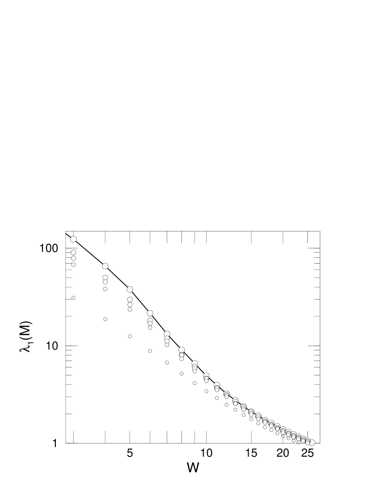
FIG. 7.: Dependence of $\lambda_{1}(M)$ on disorder $W$ for the 2D Anderson model at $E=0$ for $M=10,25,30,35$ and $50$ indicated by increasing symbol size. We use the $M=50$ data, emphasized by the solid line, as finite-size estimate of $\lambda_{1}$.

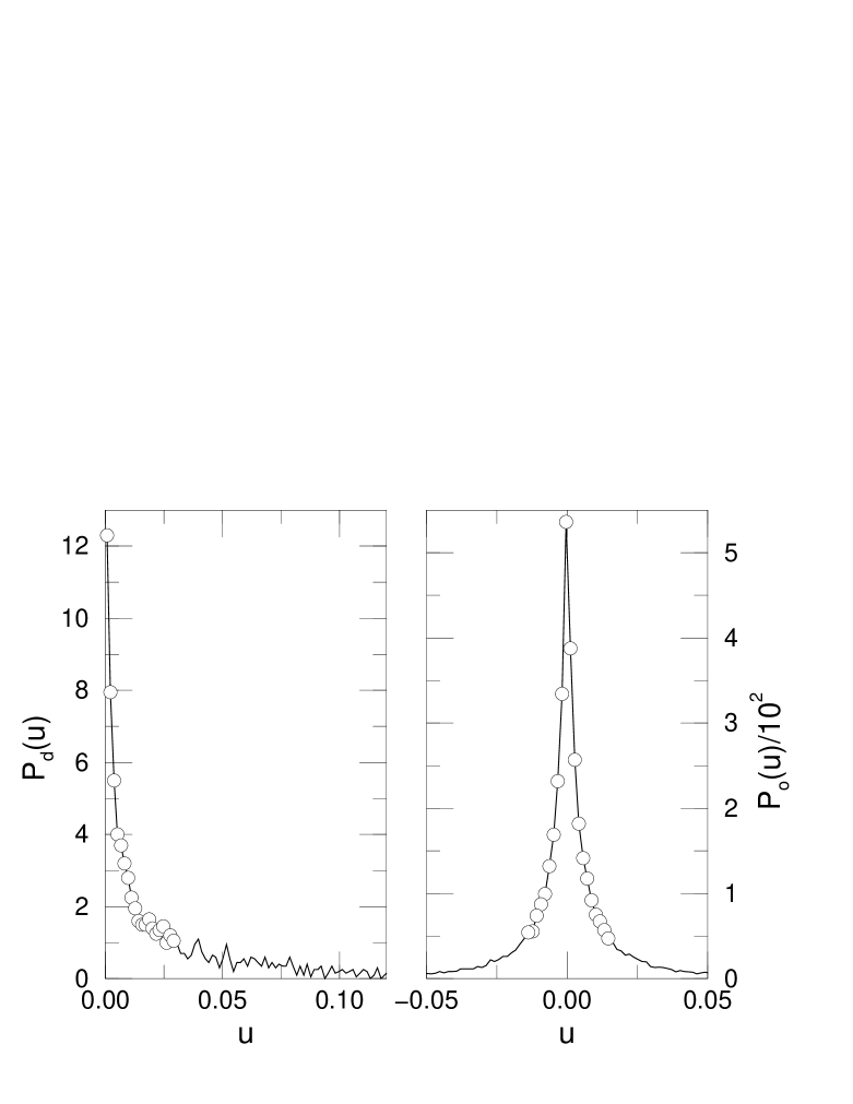
FIG. 8.: Unnormalized distribution for the diagonal (left panel) and off-diagonal (right panel) coupling matrix elements $u$ with bin width $\Delta=0.0015$ for the perturbed 2D Anderson model with $\lambda_{1}=3.1$ ($W=12$) and $M=25$. The circles indicate the 20 smallest $u$ (largest $P_{\text{o}}(u)$) for diagonal (off-diagonal) data.

FIG. 9.: Dependence of $u_{\text{abs}}$ (squares) and $u_{\text{typ}}$ (circles) on $\lambda_{1}(M)$ for the perturbed 2D Anderson model and $M=10,25,30$ and $35$ indicated by increasing symbol size. The solid lines represent the power laws $u_{\text{abs}}\sim\lambda_{1}^{-1.6}$ and $u_{\text{typ}}\sim\lambda_{1}^{-1.5}$.

FIG. 10.: Dependence of $u_{\text{abs}}$ (squares) and $u_{\text{typ}}$ (circles) on $\lambda_{1}$ for the perturbed 1D Anderson model and $M=200,300,500$ and $800$ indicated by increasing symbol size. The solid lines represent the power laws $u_{\text{abs}}\sim\lambda_{1}^{-0.48}$ and $u_{\text{typ}}\sim\lambda_{1}^{-0.59}$.

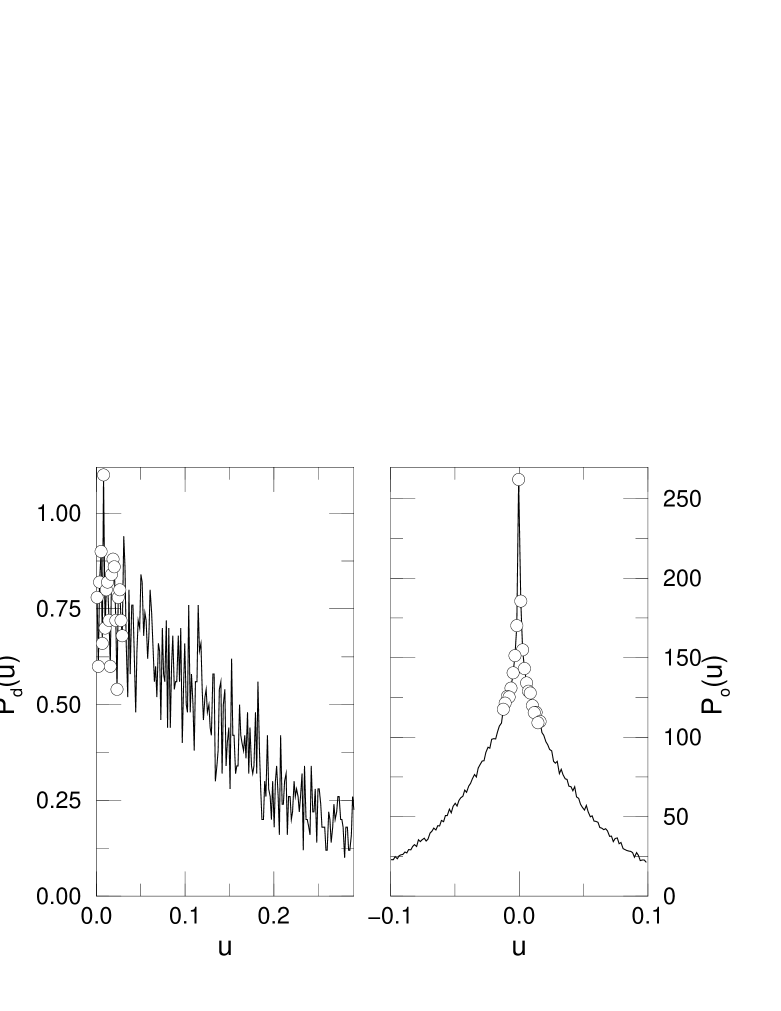
FIG. 11.: Unnormalized distribution for the diagonal (left panel) and off-diagonal (right panel) coupling matrix elements $u$ with bin width $\Delta=0.0015$ for the perturbed 1D Anderson model with $\lambda_{1}=26$ ($W=2$) and $M=200$. The circles indicate the 20 smallest $u$ (largest $P_{\text{o}}(u)$) for the diagonal (off-diagonal) data.

- [1] see, e.g., P. A. Lee and T. V. Ramakrishnan, Rev. Mod. Phys. 57, 287 (1985) and D. Belitz and T. R. Kirkpatrick, Rev. Mod. Phys. 66, 261 (1994).
- [2] E. Abrahams, P. W. Anderson, D. C. Licciardello, and T. V. Ramakrishnan, Phys. Rev. Lett. 42, 673 (1979).
- [3] S. V. Kravchenko, D. Dimonian, and M. P. Sarachik, Phys. Rev. Lett. 77, 4938 (1996).
- [4] D. L. Shepelyansky, Phys. Rev. Lett. 73, 2607 (1994); F. Borgonovi and D. L. Shepelyansky, Nonlinearity 8, 877 (1995); —, J. Phys. I France 6, 287 (1996).
- [5] D. L. Shepelyansky, Proc. Moriond Conf., Jan. 1996, cond-mat/9603086.
- [6] G. Czycholl, B. Kramer, and A. MacKinnon, Z. Phys. B 43, 5 (1981); M. Kappus and F. Wegner, Z. Phys. B 45, 15 (1981); J.-L. Pichard, J. Phys. C 19, 1519 (1986).
- [7] Y. Imry, Europhys. Lett. 30, 405 (1995).
- [8] T. Giamarchi and H. J. Schulz, Phys. Rev. B 37, 325 (1988).
- [9] Ph. Jacquod and D. L. Shepelyansky, Phys. Rev. Lett. 75, 3501 (1995).
- [10] D. Weinmann and J.-L. Pichard, Phys. Rev. Lett. 77, 1556 (1996).
- [11] K. Frahm and A. Müller-Groeling, Europhys. Lett. 32, 385 (1995).
- [12] K. Frahm, A. Müller-Groeling, and J.-L. Pichard, Phys. Rev. Lett. 76, 1509 (1996).
- [13] K. Frahm, A. Müller-Groeling, J.-L. Pichard, and D. Weinmann, Europhys. Lett. 31, 169 (1995).
- [14] F. v. Oppen, T. Wettig, and J. Müller, Phys. Rev. Lett. 76, 491 (1996).
- [15] P. H. Song and D. Kim, Phys. Rev. B 56, 12217 (1997).
- [16] D. Weinmann, A. Müller-Groeling, J.-L. Pichard, and K. Frahm, Phys. Rev. Lett. 75, 1598 (1995).
- [17] R. A. Römer and M. Schreiber, Phys. Rev. Lett. 78, 515 (1997); D. Weinmann, A. Müller-Groeling, J.-L. Pichard, and K. Frahm, Phys. Rev. Lett. 78, 4889 (1997); R. A. Römer and M. Schreiber, Phys. Rev. Lett. 78, 4890 (1997); R. A. Römer and M. Schreiber, phys. stat. sol. (b) 205, 275 (1998).
- [18] I. V. Ponomarev and P. G. Silvestrov, Phys. Rev. B 56, 3742 (1997).
- [19] S.-J. Xiong and S. N. Evangelou, preprint (1997), cond-mat/9703188.
- [20] A. MacKinnon and B. Kramer, Z. Phys. B 53, 1 (1983).
- [21] D. J. Thouless, J. Phys. C 5, 77 (1972).
- [22] Ph. Jacquod, D. L. Shepelyansky, and O. P. Sushkov, Phys. Rev. Lett. 78, 923 (1997).