[

Dephasing by time-dependent random potentials

Abstract

Diffusion of electrons in a two-dimensional system with time-dependent random potentials is investigated numerically. The correction to the conductivity due to inelastic scatterings by oscillating potentials is shown to be a universal function of the frequency $\omega$, which is consistent with the weak localization prediction $\frac{e^{2}}{3\pi^{2}\hbar}\log\omega$.

] Transport properties of the two-dimensional disordered electron systems have attracted much attention in recent years. To understand the transport properties of a random system, the concept of quantum interference plays an important role. The constructive interference of two time-reversed trajectories enhances the probability for backscattering, leading to the contribution called weak localization correction.[1, 2] Another example is the phenomenon of the sample specific reproducible conductance fluctuation,[3, 4] which is highly sensitive to the motion of a single impurity atom in the metallic region.[5, 6, 7, 8] More recently, such impurity-motion-induced conductance fluctuations have been utilized experimentally to study the detailed dynamics of impurity atom tunneling in a single two-level system in disordered metals.[9] The motion of an interstitial impurity between two energetically equivalent stability points that have different effects on the conductivity is also studied to understand the temporal fluctuations of the conductance, where one can observe $1/f$ noise.[10]

Such effects of quantum interference are suppressed in the presence of the inelastic scattering, for instance, due to the electron-phonon interaction or due to the Coulomb interaction of conduction electrons. There exists a time scale called dephasing time $\tau_{\phi}$, after which the interference effects are destroyed.[11, 12] The dephasing time is determined by the inelastic process and usually depends on the magnetic field or on the temperature. Consequently, the effect of interference can be observed experimentally by controlling these parameters .

In this paper, we study the effect of dynamically fluctuating potentials on the conductivity by solving the time-dependent Schrödinger equation numerically. We adopt here the formula for solving the time-dependent Schrödinger equation proposed by Suzuki,[13, 14, 15, 16, 17, 18] which make it possible to deal numerically with the time-dependent potential on the sufficiently large system of two-dimensional lattice. We observe the second moment of the wave packet, which gives information about extension of the wave packet. We then evaluate the conductivity and discuss how the conductivity depends on the motion of potentials, in particular, on the frequency of potentials.

In order to solve numerically the time-dependent Schrödinger equations, we adopt the method based on the higher-order decomposition of exponential operators.[13, 19] The basic formula we have used is the fourth-order decomposition of exponential operators:

$$\exp[x(A_{1}\ +\ A_{2}\ +\ \cdots\ +\ A_{q})]$$ (1)

$$= S(xp)S\left(x(1-2p)\right)S(xp)+O(x^{5}),$$ (2)

where

$$S(x)\ =\ e^{xA_{1}/2}e^{xA_{2}/2}\cdots e^{xA_{q-1}/2}e^{xA_{q}}e^{xA_{q-1}/2}\cdots e^{xA_{1}/2},$$ (3)

and the parameter $p$ is given by $p\ =\ (2-\sqrt[3]{2})^{-1}$. Here $A_{1},\dots,A_{q}$ are arbitrary operators.

We consider the tight-binding Hamiltonian with time-dependent potential $\varepsilon_{i}(t)$ on the two-dimensional square lattice:

$$H(t)\ =\ -\ V\sum_{(i,j)}C_{i}^{\dagger}C_{j}\ +\ \sum_{i}\varepsilon_{i}(t)C_{i}^{\dagger}C_{i},$$ (4)

where $C^{\dagger}_{i}(C_{i})$ denotes a creation (annihilation) operator of an electron at the site $i$ and $(i,j)$ is the nearest neighbor site. We then decompose this Hamiltonian into five parts as described in ref. [20], namely,

$$H(t) = \sum_{n=1}^{4}H_{n}\ +\ H_{5}(t),$$ (5)

$$H_{1} \equiv V\sum_{r_{x}\in{\rm odd}}\sum_{r_{y}}C_{\vec{r}+\hat{x}}^{\dagger}C_{\vec{r}}+{\rm h.c.},$$ (6)

$$H_{2} \equiv V\sum_{r_{x}\in{\rm even}}\sum_{r_{y}}C_{\vec{r}+\hat{x}}^{\dagger}C_{\vec{r}}+{\rm h.c.},$$ (7)

$$H_{3} \equiv V\sum_{r_{x}}\sum_{r_{y}\in{\rm odd}}C_{\vec{r}+\hat{y}}^{\dagger}C_{\vec{r}}+{\rm h.c.},$$ (8)

$$H_{4} \equiv V\sum_{r_{x}}\sum_{r_{y}\in{\rm even}}C_{\vec{r}+\hat{y}}^{\dagger}C_{\vec{r}}+{\rm h.c.},$$ (9)

$$H_{5}(t) \equiv \sum_{\vec{r}}\varepsilon_{\vec{r}}(t)C_{\vec{r}}^{\dagger}C_{\vec{r}},$$ (10)

where $\hat{x}(\hat{y})$ denotes the unit vector in the $x(y)-$direction and $r_{x}(r_{y})$ the $x(y)$ component of the position vector $\vec{r}$ of the sites. All the length-scales are measured in units of the lattice constant $a_{0}$. Each Hamiltonian $H_{n}$ consists of operators which commute with each other, hence we can obtain the analytical expressions for $\exp(-{\rm i}H_{n}t/\hbar)$ by diagonalizing two by two matrices.

The state vector $|\psi(t\ +\ \delta t)\rangle$ at time $t\ +\ \delta t$ is obtained as

$$|\psi(t\ +\ \delta t)\rangle\ =\ U(t\ +\ \delta t,t)|\psi(t)\rangle,$$ (11)

where the time-development operator $U(t\ +\ \delta t,t)$ is defined by

$$U(t\ +\ \delta t,t)\ =\ T\left(\exp{\left[-\frac{i}{\hbar}\int_{t}^{t\ +\ \delta t}H(s)ds\right]}\right),$$ (12)

with $T$ the time-ordering operator. Using the formula proposed by Suzuki,[17] this ordered exponential can be expressed by an ordinary exponential operator as

$$U(t\ +\ \delta t,t)\ =\ \exp{\left[\delta t(-\frac{i}{\hbar}H(t)\ +\ {\cal T})\right]},$$ (13)

where the super-operator $\cal T$ is defined by

$$F(t)e^{\delta t{\cal T}}G(t)\ =\ F(t\ +\ \delta t)G(t).$$ (14)

Using formula (2) and (13), the time-development operator (12) is decomposed as the product of exponential operators;[17]

$$U(t+\delta t,t)\ = S_{2}(-{\rm i}\delta tp/\hbar,\ t+(1-p/2)\delta t)$$ (15)

$$\times S_{2}(-{\rm i}\delta t(1-2p)/\hbar,\ t+\delta t/2)$$ (16)

$$\times S_{2}(-{\rm i}\delta tp/\hbar,\ t+p\delta t/2)$$ (17)

$$+ O(\delta t^{5})$$ (18)

with

$$S_{2}(x,t) \equiv {\rm e}^{xH_{1}/2}{\rm e}^{xH_{2}/2}\cdots{\rm e}^{xH_{4}/2}{\rm e}^{xH_{5}(t)}$$ (19)

$$\times {\rm e}^{xH_{4}/2}\cdots{\rm e}^{xH_{2}/2}{\rm e}^{xH_{1}/2}.$$ (20)

In order to consider the time evolution of the wave packet with fixed energy $E$, we have carried out a numerical diagonalization of a subsystem $H_{N_{0}}$ whose size is $N_{0}$ by $N_{0}$, located at the center of the whole system and have chosen an eigenstate of $H_{N_{0}}$ with eigenvalue $E_{N_{0}}\approx E$ as the initial wave packet.

The quantity we observe is the second moment of the wave packet $\langle r^{2}(t)\rangle_{c}$ defined by

$$\langle r^{2}(t)\rangle_{c}\equiv\langle|\vec{r}(t)|^{2}\rangle-\langle\vec{r}(t)\rangle^{2}$$ (21)

with

$$\langle r^{2}(t)\rangle\equiv\int{\rm d}\Omega r^{d-1}{\rm d}rr^{2}|\psi(\vec{r},t)|^{2},$$ (22)

where $\psi(\vec{r},t)$ denotes the wave function at time $t$, and $d$ the dimensionality of the system. If the wave function extends throughout the whole system, the second moment is expected to grow in proportion to time $t$

$$\langle r^{2}\rangle_{c}\ =\ 2dDt.$$ (23)

Here, the coefficient $D$ denotes the diffusion coefficient. In contrast, if the wave function is localized, it is clear that the second moment remains finite in the limit $t\rightarrow\infty$.[19] In the metallic region the Einstein relation

$$\sigma\ =\ e^{2}\rho(E_{\mbox{F}})D$$ (24)

relates the conductivity $\sigma$ to the diffusion constant, where $\rho(E_{\mbox{F}})$ is the density of state at Fermi energy $E_{\mbox{F}}$.

In order to take into account the effect of moving potential, we assume that the site-potentials take the form:

$$\varepsilon_{\vec{r}}(t)\ =\ \varepsilon_{\vec{r}}(0)\cos{\left[\omega t+\theta\left(\vec{r}\right)\right]},$$ (25)

where $\omega$ is the frequency. Effects of scattering from impurities are introduced through randomness of site energy $\varepsilon_{\vec{r}}(0)$ and phase $\theta(\vec{r})$ at $t\ =\ 0$ distributed uniformly in the regions,

$$|\varepsilon_{\vec{r}}(0)| < W/2,$$ (26)

$$|\theta(\vec{r})| < \pi.$$ (27)

We consider the adiabatic case $\omega\ll V/\hbar$, where impurities move slower than electrons.

We have calculated the second moment of the wave packet $\langle r^{2}\rangle_{c}$ at various random potential strength. The size of the systems are 500 by 500 for the energies $E_{\mbox{F}}/V\ =\ -1$. We have carried out an exact diagonalization for the 20 by 20 subsystem at the center of the system and taken the eigenfunction of the subsystem whose eigenvalue is closest to the given energy $E_{\mbox{F}}$ as the initial wave packet. By this procedure we can simulate the diffusion of the wave packet whose energy is approximately equal to $E_{\mbox{F}}$. The single time step $\delta t$ is taken to be $0.2(\hbar/V)$ in the simulation. With this choice of $\delta t$, fluctuations of the expectation value of the Hamiltonian $\langle H\rangle\equiv\langle\psi(t)|H|\psi(t)\rangle$ for $\omega=0$ can be safely neglected [19, 20] throughout our simulations ($t\leq 2000(\hbar/V)$).

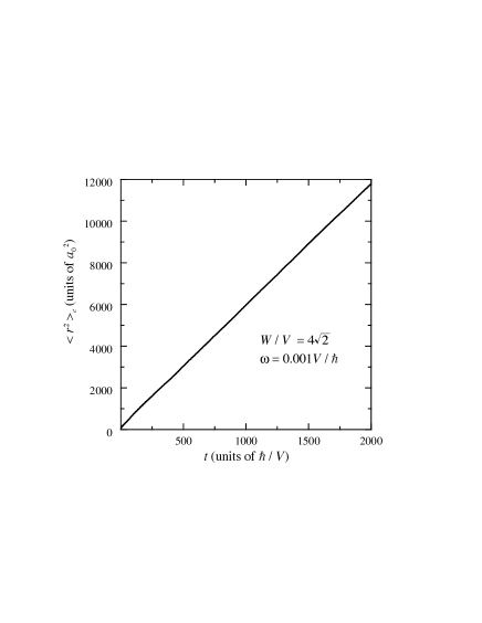
FIG. 1.:

Fig. 1 gives an example of the calculated second moment for $\omega\ =\ 10^{-3}V/\hbar,$ $W/V\ =\ 4\sqrt{2}$. The second moment is proportional to the time in a wide range up to $2\times 10^{3}\hbar/V$. We can evaluate the diffusion constant of this system from Eq. (23) with least square fit to these data and obtain the diffusion constant of the sample to be $D\ =\ 1.46a^{2}V/\hbar$. In the actual simulation, the quantities $\langle r^{2}\rangle_{c}$ are averaged over at least five samples of random potential distribution. The density of states $\rho(E_{\mbox{F}})$ in Eq. (24) is evaluated from the direct diagonalization of the two-dimensional lattice model for 40 by 40 sites for $\omega\ =\ 0$, and an average over 100 samples is performed. We have obtained that $\rho(E_{\mbox{F}})a_{0}^{2}V\ =\ 0.292,\ 0.291,\ 0.281,$ and $0.251$ for $W/V\ =\ 2,\ 2\sqrt{2},\ 4,$ and $4\sqrt{2}$, respectively.

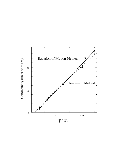
FIG. 2.:

In Fig. 2, we show the conductance for $\omega\ =\ 0$ obtained by the present method, and compare it with that calculated by a conventional recursive Green’s function method.[21] The results show that two methods agree fairly well with each other. We can also see the conductivity is proportional to $(W/V)^{-2}$ in a wide range of $W/V$.

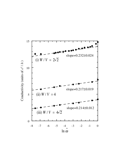
FIG. 3.:

In Fig. 3 we show examples of the conductivity as the function of $\ln{\tilde{\omega}}$ for $W/V\ =\ 2\sqrt{2},4,$ and $4\sqrt{2}$, where $\tilde{\omega}\ =\ \omega/(V/\hbar)$. The conductivity linearly depends on $\ln{\tilde{\omega}}$ as

$$\sigma\ =\ A\ln{\tilde{\omega}}\ +\ \sigma(0).$$ (28)

The coefficients $A(\approx 0.22)$ calculated by the least square fit to the averaged conductivity, are almost the same among these three different disorder cases, although the conductivity $\sigma(0)$ for $\omega\ =\ 0$ is significantly different from each other.

To interpret the above universal correction due to frequency $\omega$, we recall the weak localization correction,

$$\delta\sigma=-\frac{e^{2}}{2\pi^{2}\hbar}\ln{\frac{\tau_{\phi}}{\tau}},$$ (29)

where $\tau_{\phi}$ is the dephasing time, and $\tau$ the elastic scattering time. The $\omega$ dependence of $\tau_{\phi}$ in the kicked rotator problem[22] as well as that in the one-dimensional disordered system [23] in the presence of noise is estimated to be $\sim\omega^{-2/3}$. Then the weak localization correction $\delta\sigma$ [24, 25] is estimated to be

$$\delta\sigma=\frac{2}{3\pi}\frac{e^{2}}{h}\ln{\frac{\omega}{\omega_{0}}}.$$ (30)

The pre-factor $2/3\pi\ =\ 0.212\dots$ of the $\ln{\omega}$ term agrees with the numerical calculation shown in Fig. 3, which is universal and independent of the potential strength $W$. Note that this $\omega$-dependence is also observed in the case of low energy phonon scattering.[26]

To justify our argument, the condition $\tau\ll\tau_{\phi}$ is necessary. This is why the conductivity deviates from the $\log\omega$ behavior in large $\omega$ region, where $\tau$ is the order of $\tau_{\phi}$. We also see the deviation from the $\log\omega$ behavior in a small $\omega$ region. In this case, $\omega$ is too small for the potential to be changed in a finite time where our simulation has been performed.

In conclusion, we have analyzed the weak localization effect in the two-dimensional system with time-dependent random potentials using the equation-of-motion method. It has been shown numerically that the weak localization correction to the conductivity due to the fluctuating potentials takes universal value independent of the random potential strength $W$. The correction term agrees with the formula $\delta\sigma\ =\ \frac{2}{3\pi}\frac{e^{2}}{h}\ln{\frac{\omega}{\omega_{0}}}$, proposed for the inelastic scattering by moving impurities. Our results will open a new way to incorporate the dephasing mechanism in numerical simulations.

One of the authors (T. N.) acknowledges the financial support from the Proposal-Based Advanced Industrial Technology R&D Program of the NEDO. Numerical calculations were performed on FACOM VPP500 in Supercomputer Center, Institute for Solid State Physics, University of Tokyo.

Fig. 1: An example of the second moment as the function of time for $\omega\ =\ 10^{-3}V/\hbar,$ $W/V\ =\ 4\sqrt{2},$ and $E_{\mbox{F}}/V\ =\ -1$. The solid line corresponds to $D\ =\ 1.46a^{2}V/\hbar$.
Fig. 2: Conductivity obtained by the equation-of-motion method (solid line) for $\omega\ =\ 0$. The dashed line corresponds to the conductance calculated by the recursive Green’s function method.
Fig. 3: The calculated conductivity of the two-dimensional system with time dependent impurity potential for (i) $W/V\ =\ 2\sqrt{2}$, (ii)$W/V\ =\ 4$, and (iii) $W/V\ =\ 4\sqrt{2}$. The solid lines indicate the corrections $\delta\sigma\ =\ 0.232\frac{e^{2}}{h}\ln{\tilde{\omega}}$, $\delta\sigma\ =\ 0.217\frac{e^{2}}{h}\ln{\tilde{\omega}}$, and $\delta\sigma\ =\ 0.214\frac{e^{2}}{h}\ln{\tilde{\omega}}$, respectively.

REFERENCES

- [1] E. Abrahams, P. W. Anderson, D. C. Licciardello and T. V. Ramakrishnan, Phys. Rev. Lett. 42 (1979) 673.
- [2] L. P. Gorkov, A. I. Larkin, and D. E. Khmelnitskii, Pis’ma Zh. Eksp. Teor. Fiz. 30 (1979) 248 [Sov. Phys. JETP 30 (1979) 288].
- [3] P. A. Lee and A. D. Stone, Phys. Rev. Lett. ,55 (1985) 1622.
- [4] B. L. Alt’shuler, Pis’ma Zh. Eksp. Teor. Fiz. 41 (1985) 530 [JETP Lett. 41 (1985) 648].
- [5] S. Feng, P. A. Lee, and A. D. Stone, Phys. Rev. Lett. ,56 (1986) 1960.
- [6] S. Feng, J. -L. Pichard and F. Zeng, Phys. Rev. B48 (1993) 2529.
- [7] S. J. Klepper, O. Millo, M. W. Keller, D. E. Prober, and R. N. Sacks, Phys. Rev. B44 (1991) 8380.
- [8] D. E. Beulter, T. L. Meisenheimer, and N. Giordano, Phys. Rev. Lett. 58 (1987) 1240.
- [9] N. M. Zimmerman, B. Golding, and W. H. Haemmerle, Phys. Rev. Lett. 67 (1991) 1322.
- [10] M. B. Weissmann, Rev. Mod. Phys. 60 (1988) 537.
- [11] B. L. Al’tshuler, A. G. Aronov, and P. A. Lee, Phys. Rev. Lett. 44 (1980) 1288.
- [12] H. Fukuyama, J. Phys. Soc. Japan 48 (1980) 2169.
- [13] M. Suzuki, Phys. Lett. A146 (1990) 319.
- [14] M. Suzuki, J. Math. Phys. 32 (1991) 400.
- [15] M. Suzuki, J. Phys Soc. Jpn. 61 (1992) 3015.
- [16] M. Suzuki, Phys. Lett. A165 (1992) 387.
- [17] M. Suzuki, Proc. Jpn Acad. 69, Ser. B (1993) 161.
- [18] M. Suzuki, Commun. Math. Phys. 163 (1994) 491.
- [19] H. De Raedt, Computer Phys. Rep. 7 (1987) 1; Europhys. Lett. 3 (1987) 139.
- [20] T. Kawarabayashi and T. Ohtsuki, Phys. Rev. B51 (1995) 10897; B53 (1996) 6975.
- [21] T. Ando, Phys. Rev. B44 (1991) 8017.
- [22] S. Fishman and D. L. Shepelyansky, Europhys. Lett. 16 (1991) 643.
- [23] F. Borgonovi, and D. L. Shepelyansky, Phys. Rev. E51 (1995) 1026.
- [24] G. Bergmann, Phys. Rep. 107 (1984) 1.
- [25] S. Hikami, A. Larkin and Y. Nagaoka: Prog. Theor. Phys. 63 (1980) 707.
- [26] In the case of low energy phonon scattering, the dephasing time is estimated to be where is the phonon velocity. Assuming we obtain . See, M. J. Stephen, Phys. Rev. B36 (1987) 5663. A. A. Golubentsev, Zh. Eksp. Teor. Fiz. 86 (1984) 47. [Sov. Phys. JETP 59 (1984) 26.]
Fig. 1:
An example of the second moment as the function of time for
and
. The solid line corresponds
to .
Fig. 2:
Conductivity obtained by the equation-of-motion
method (solid line) for . The dashed line corresponds to
the conductance calculated by the recursive Green’s function method.
Fig. 3:
The calculated conductivity of the two-dimensional system with time
dependent impurity potential for (i) , (ii),
and (iii) .
The solid lines indicate the corrections
,
,
and ,
respectively.