[

On Nonlinear Diffusion with Multiplicative Noise

Abstract

Nonlinear diffusion is studied in the presence of multiplicative noise. The nonlinearity can be viewed as a “wall” limiting the motion of the diffusing field. A dynamic phase transition occurs when the system “unbinds” from the wall. Two different universality classes, corresponding to the cases of an “upper” and a “lower” wall, are identified and their critical properties are characterized. While the lower wall problem can be understood by applying the knowledge of linear diffusion with multiplicative noise, the upper wall problem exhibits an anomaly due to nontrivial dynamics in the vicinity of the wall. Broad power-law distribution is obtained throughout the bound phase.

PACS: 64.60.Ht, 02.50.-r, 47.20.Ky

]

The diffusion equation with multiplicative noise has been used as a paradigm to describe a large class of nonequilibrium dynamical processes [1] ranging from light propagation in random media to wealth fluctuations in economic systems. In this paper, we study the effect of nonlinearities, which inevitably occur in such processes due to the existence of characteristic scales of the diffusing fields. For instance, the growth of a population is bounded from above by a characteristic density determined by the competition of resources [2], and an investor’s wealth can be taken as bounded from below by a fixed income source [3]. At sufficiently coarse grained scales, these effects may be captured by the following nonlinear diffusion equation with multiplicative noise,

$${\partial}_{t}n={\bf\nabla}^{2}n+a\,n-b\,n^{1+p}+n({\bf x},t)\,\eta({\bf x},t)$$ (1)

where $a$ and $b$ are constants, $p$ specifies the degree of nonlinearity, and $\eta({\bf x},t)$ is a Gaussian noise with zero mean and the variance $\left\langle\eta({\bf x},t)\eta({\bf x}^{\prime},t^{\prime})\right\rangle=2D\,\delta({\bf x}-{\bf x}^{\prime})\,\delta(t-t^{\prime})$. Note that Eq. (1) should be interpreted either in the Ito or Stratanovich sense [4], depending on the details of the specific process being considered. We shall fix the nonlinearity coefficient to be $b=p$ from here on, so that for $p>0$, the nonlinear term acts like a soft upper wall preventing $n({\bf x},t)$ from reaching large values even if $a$ is large and positive, while for $p<0$, the nonlinear term acts like a soft lower wall repelling $n({\bf x},t)$ from approaching zero even for large and negative $a$’s. The specific choice of $p$ depends on the symmetries and constraints of the system. The limits $p\rightarrow\pm\infty$ mimic the effect of hard upper/lower walls and are also of interest.

It will be convenient to cast the upper/lower wall problems in a more “symmetric” form. By making use of the Cole-Hopf transform, $h({\bf x},t)=\log n({\bf x},t)$, we have

$$\partial_{t}h=\mbox{\boldmath$\nabla$}^{2}h+(\mbox{\boldmath$\nabla$}h)^{2}+(a-a_{0})-pe^{ph}+\eta({\bf x},t),$$ (2)

which is a Langevin equation similar to the KPZ equation describing the kinetic roughening of a growing interface $h$ [5, 6], with an additional drift term $a-a_{0}$ ($a_{0}=0$ for Stratanovich dynamics and $a_{0}=D$ for Ito dynamics [4]), and an “exponential wall” at $h\approx 0$. Thus a wall in the diffusion problem corresponds to a wall also in the interface problem. Eq. (2) shows that the sign of $p$ determines the orientation of the wall while the magnitude of $p$ describes the hardness of the wall. In the interface representation, it is clear that for large positive [negative] $a$’s, the system is pushed against the upper [lower] wall, while for large negative [positive] $a$’s, the system is pushed away from the wall to $h=-\infty$ [$h=+\infty$], corresponding to $n=0$ [$n=\infty$]. A critical point separates the two regimes where the system “unbinds” from the wall. In this paper, we study the nature of this dynamic unbinding transition for walls characterized by different $p$’s. We will show that while the soft and hard walls yield the same critical phenomena, the upper and lower walls yield two different universality classes.

We start with a review of the exactly solvable “zero-dimensional” (single-site) version of Eqs. (1) and (2) [7]. Without spatial couplings, the stationary probability distribution $\widetilde{P}(h)$ of Eq. (2) is simply

$$\widetilde{P}(h)\propto\exp\left[\frac{a-a_{0}}{D}h\right]\cdot\exp\left[-\frac{1}{D}e^{ph}\right],$$ (3)

where the second exponential merely enforces the constraint of the wall, suppressing $\widetilde{P}$ for $h>0$ [$h<0$] if $p>0$ [$p<0$]. From (3), the stationary distribution of $n$ is easily obtained using the relation $P(n)=n^{-1}\,\widetilde{P}(\log n)$, yielding $P(n)\propto n^{[(a-a_{0})/D]-1}\exp(-n^{p}/D)$. Note that the distribution functions are normalizable as long as $(a-a_{0})\cdotp>0$, and hence a power-law distribution in $n$ is obtained for a large range of parameter values. [A similar result was obtained previously for the case of a hard lower wall [8, 9]; it was proposed as an explanation of the observed power-law distribution of wealth [10].]

As $a\to a_{0}^{\pm}$, the average $h$ diverges according to Eq. (3) as $\langle h\rangle\sim\mp|a-a_{0}|^{-1}$ for the upper/lower wall, indicating the onset of an “unbinding transition” of $h$ from the wall. This transition can be characterized quantitatively by singularities in moments of $n$. From $P(n)$, we find for the upper wall problem $\langle n^{m}\rangle\sim(a-a_{0})^{{\beta}_{m}}$ and ${\beta}_{m}=1$ for all integer $m$’s. The distribution collapses towards $P(n)=\delta(n)$ as $a\to a_{0}^{+}$. For the lower wall, $\langle n^{m}\rangle$ diverge as $a\rightarrow a_{0}^{-}$ since $P(n)$ has no upper cutoff. It is convenient to characterize the phase transition in this case by monitoring $\bar{n}\equiv 1/n$. One finds $\langle\bar{n}^{m}\rangle\sim(a_{0}-a)^{\bar{\beta}_{m}}$, with $\bar{\beta}_{m}=1$ also. The symmetry between the upper and lower wall problems is evident from the $h\rightarrow-h$ symmetry of Eq. (2) in the absence of spatial couplings. Note that the asymptotic critical properties given above are independent of the parameter $p$, indicating that in the vicinity of the unbinding transition, where $\langle n\rangle$ approaches zero or infinity (or as $\langle h\rangle\to\mp\infty$), the detailed form of the wall at finite $n$ (or at $h\approx 0$) is irrelevant.

Time-dependent properties of the system can be obtained by solving the full Fokker-Planck equation [4, 7]. Qualitative features can be obtained alternatively by considering the simpler Langevin equation for $h(t)$. We illustrate the solution by analyzing the problem with a lower wall $(p<0)$. For $a<a_{0}$, $h$ is confined to the range $0\lesssim h\lesssim\delta h$, where $\delta h\sim(a_{0}-a)^{-1}$ is the scale of typical fluctuations in $h$. Right at the critical point $a=a_{0}$, $\delta h$ diverges, i.e., $\delta h(t)\rightarrow\infty$ as $t\rightarrow\infty$. The form of $\delta h(t)$ is dictated by the equation of motion at the critical point, $\partial_{t}h=-p\,e^{ph}+\eta(t).$ $\delta h(t)$ must be at least of $O(t^{1/2})$ due to the random forcing $\eta$; the presence of the wall can only speed up the motion away from the wall. On the other hand, as $h$ drifts far away from the wall, it should not be affected by the wall. Thus $\delta h(t)\sim t^{1/2}$ at the transition, with the distribution given by the scaling form

$$\widetilde{P}(h,t)=\left(\delta h\right)^{-1}\,g\left[h/\delta h(t)\right]\quad{\rm for}\quad ph<0.$$ (4)

In (4), the factor $\left(\delta h(t)\right)^{-1}$ provides the proper normalization, and $g(y)$ is a scaling function with the limiting behaviors $g(y)\approx{\rm const}$ for $|y|\ll 1$ and $g(y)\rightarrow 0$ for $|y|\gg 1$. The distribution $P(n,t)$ follows from (4), yielding $\langle n^{m}\rangle\sim\delta h\sim t^{1/2}$ for all positive moments $m$.

We now proceed to characterize the behavior of the system in arbitrary spatial dimension $d$. This is accomplished by generalizing the above zero-dimensional picture and utilizing the known properties of the KPZ equation in finite dimensions [5]. The Cole-Hopf transformation has already been exploited in Ref. [11] to derive some properties of the system with a soft upper wall $(p>0)$. Some of the arguments there (but not all [12]) can be generalized also to the case of a lower wall.

Close to the critical point, $h({\bf x},t)$ is on average far from the wall, and the main source of fluctuation comes from the stochastic KPZ equation without walls (for all length scales below the correlation length $\xi$). The scaling properties of the KPZ equation can be described in terms of the dynamic exponent $z$ alone [5]: the typical correlation time is $\tau\sim\xi^{z}$ and typical height fluctuation is $\delta h\sim\xi^{2-z}$. These properties yield the scaling form for the additive renormalization $\langle(\mbox{\boldmath$\nabla$}h)^{2}\rangle$ of the bare drift $(a-a_{0})$, with $\langle(\mbox{\boldmath$\nabla$}h)^{2}\rangle=a_{1}-a_{2}(\xi)$, where $a_{1}\propto D$ is a constant and $a_{2}(\xi)\sim(\delta h/\xi)^{2}\sim\xi^{-1/(2z-2)}$. Thus one obtains the important result $\xi\sim|a-a_{c}|^{-\nu}$ with $a_{c}=a_{0}-a_{1}$ [13] and $\nu=1/(2z-2)$ for both the upper and lower wall. In particular, in one dimension where it is known exactly that $z=3/2$, we have $\nu=1$, while in $d=2$, $z\approx 1.60$ yields $\nu\approx 0.83$. The exponents $\nu$ and $z$ can be used to relate the exponents $\beta$ [$\overline{\beta}$] and $\theta$[$\overline{\theta}$] which describe the behavior of the “order parameter” $n$ [$\overline{n}=n^{-1}$] close to the critical point for the problem with an upper [lower] wall. From the definitions $\left\langle n^{m}\right\rangle\sim\left|a-a_{c}\right|^{\beta_{m}}$ and $\left\langle n^{m}\right\rangle\sim t^{-\theta_{m}}$ at $a=a_{c}$, it follows that $\theta_{m}=\beta_{m}/(\nu z)$; similarly, $\overline{\theta}_{m}=\overline{\beta}_{m}/(\nu z)$.

To find the exponents $\beta$ and $\theta$, we first perform a naive scaling analysis. Let us assume that the probability distribution $\widetilde{P}(h,t)$ at the critical point is still given by the scaling form (4) as in the zero-dimensional case, but with $\delta h(\tau)\sim\tau^{\omega}$ where $\omega=(2-z)/z$ in $d>0$. We then find $\langle n^{m}\rangle_{{\rm upper}}\sim\langle\bar{n}^{m}\rangle_{{\rm lower}}\sim\delta h$ as before, yielding $\theta_{m}=\overline{\theta}_{m}=\omega=(2-z)/z$ and $\beta_{m}=\overline{\beta}_{m}=(2-z)/(2z-2)$ for all $m$’s. These exponents take on the value $\theta=1/3$, $\beta=1/2$ in 1d and $\theta\approx 0.25$ and $\beta\approx 0.33$ in 2d.

In the above analysis, we have not distinguished between systems with a lower or upper wall. On the other hand, it is evident that the equation of motion (2) for $p>0$ and $p<0$ are different in finite $d$ due to the presence of the nonlinear term $(\mbox{\boldmath$\nabla$}h)^{2}$. Thus the problems with upper and lower wall can no longer be mapped onto each other. In order to see whether the orientation of the wall is relevant to the critical behaviors, and whether the above scaling ansatz is correct, we perform a numerical simulation in one spatial dimension. We expose now the algorithm and the main results.

To speed up the computations, we use a discrete model which, in the absence of walls, belongs to the KPZ universality class [6]. This model is similar to that of ballistic deposition: At each point $x$ of a one dimensional lattice of size $L$, we define a continuous height variable, $h_{t}(x)$. At every time step a new variable $h^{\prime}(x)=h_{t}(x)+a+\eta_{t}(x)$ is obtained, with $\eta_{t}(x)$ being a random number uniformly distributed in the interval $[0,1]$. The value of $h$ is updated simultaneously according to the rule $h_{t+1}(x)=\max\left[h^{\prime}(x\pm 1)+\gamma,\,h^{\prime}(x,t)\right]$, where $\gamma=0.1$ is a fixed constant, and periodic boundary condition is applied. The parameter $a$ controls the average drift of the system and is the only tunning parameter in this model. A hard wall at $h=0$ is introduced by including the additional rule $h_{t}(x)=\min\left[h_{t}(x),0\right]$ for an upper wall or $h_{t}(x)=\max\left[h_{t}(x),0\right]$ for a lower wall.

We describe first the results for an upper wall. The first step to studying critical properties is to locate the critical point accurately. Starting with the initial condition, $h_{0}(x)=0$ for all $x$, we let the system evolve long enough so that a stationary state is reached ($\sim 10^{5}$ time steps are typically required for system size of $L\sim 10^{3}$). To compute any magnitude we average over up to 1000 independent runs. For a given size $L$, the critical point $a_{c}(L)$ is taken as the first value of $a$ for which the steady state value $\left\langle n\right\rangle=\left\langle\exp(h)\right\rangle$ becomes indistinguishable from zero as $a$ is decreased. A plot of $a_{c}(L)$ vs $1/L$ is shown in Fig. 1(a). Linearity of the data suggests $\nu\approx 1.$ Extrapolating to $L\rightarrow\infty$, we get $a_{c}\approx-1.5750$. The scaling of $\left\langle n\right\rangle$ and $\left\langle n^{2}\right\rangle$ upon approaching the critical point $a_{c}(L)$ are shown in Fig. 1(b) for $L=400$. We obtain the exponents $\beta_{1}\approx\beta_{2}=1.50\pm 0.15$. In Fig. 1(b), we plot $\langle n(t)\rangle$ and $\langle n^{2}(t)\rangle$ vs. $t$ at $a=a_{c}$, and find $\theta_{1}\approx\theta_{2}=1.10\pm 0.12$.

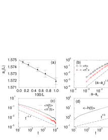
FIG. 1.: Results with an upper wall: (a) Size dependence of the critical point $a_{c}(L)$; (b) first two moments of the spatially-averaged $n$ vs. $a-a_{c}$ in the steady state; (c) time dependence of $\langle n\rangle$ and $\langle n^{2}\rangle$ at $a=a_{c}$; (d) $\langle-h(t)\rangle$ at $a=a_{c}$.

The scaling of $\langle h\rangle$ at $a=a_{c}$ is shown in Fig. 1(d). We find the exponent $\omega\approx 0.33$. To compute the dynamic exponent $z$, we perform a slightly different simulation [15]: We take as initial condition a state in which $h$ is a large negative constant at every lattice point except for the origin where $h=0$. The spreading of this “localized seed” is followed, and from the time evolution of the average size of the “infected region”, we find $z=1.50\pm 0.05$. All the measured exponents coincide, within numerical accuracy, with those computed previously [11] for Eq. (1) with $p=1,2$, i.e., soft walls. This indicates that the introduction of an upper soft or a hard wall to a model belonging to the KPZ universality class yields the same critical behavior. As found in Ref. [11], the exponents $\nu$ and $z$ agree with the result of the scaling analysis. Also the scaling relation $\theta_{m}=\beta_{m}/(\nu z)$ [11, 15] is satisfied. However, the values of $\beta$ and $\theta$ are significantly different from those derived above using the naive scaling analysis.

We next describe the results for a lower wall. Following the same analysis procedure for the “order parameter” $\left\langle\bar{n}\right\rangle=\left\langle\exp\left(-h\right)\right\rangle$, we obtain the critical point at $a_{c}\approx-1.5743$, and $\nu\approx 1$ (see Fig. 2(a)). From Fig. 2(b), we find $\bar{\beta}_{1}\approx\bar{\beta}_{2}=0.48\pm 0.05$ [12] and from Figs. 2(c) and 2(d), we find $\bar{\theta}_{1}\approx\bar{\theta}_{2}=0.32\pm 0.03$, $\omega=0.33\pm 0.04$. The dynamical exponent $z\approx 1.5$ is again determined using the seed-spreading method (a suitable initial condition is $h(x)=0$ for all $x$ except for the origin where $h(0)>0$). Note that in contrast to the case with an upper wall, all of the measured exponents here are consistent with the expected results based on the naive scaling analysis, including the values of $\bar{\beta}$ and $\bar{\theta}$. The clear difference between $\beta,\theta$ and $\bar{\beta},\bar{\theta}$ indicate that problems with upper and lower walls belong to different universality classes.

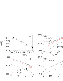
FIG. 2.: Results with a lower wall: (a) Size dependence of the critical point $a_{c}(L)$; (b) first two moments of the spatially-averaged $\bar{n}$ vs. $a_{c}-a$ in the steady state; (c) time dependence of $\langle\bar{n}\rangle$ and $\langle\bar{n}^{2}\rangle$ at $a=a_{c}$; (d) $\langle h(t)\rangle$ at $a=a_{c}$.

As the fluctuations in $\langle h(t)\rangle$ obey the same scaling law ($\omega\approx 0.33$) for both the upper and lower wall problems (see Figs. 1(d) and 2(d)), differences in the scaling of $\langle n^{m}\rangle_{{\rm upper}}$ and $\langle\bar{n}^{m}\rangle_{{\rm lower}}$ must result from differences in the shape of the distribution $\widetilde{P}(h,t)$, or more specifically, in the form of the scaling functions $g(h/t^{\omega})$ defined in Eq. (4). Our numerical results suggest that the zero-dimensional behavior of $g(y)\approx{\rm const}$ for $|y|\lesssim 1$ and $g(y)\rightarrow 0$ for $y\gg 1$ is obtained in 1d for the lower wall problem only. The numerically obtained forms of the scaling function $g(h/t^{1/3})$ for the upper and lower wall are presented in Fig. 3(a) and Fig. 3(b) respectively. Note that for large $|h|/t^{1/3}$, the distribution function drops off sharply (approximately exponentially) for both cases. Thus the assumed form for the scaling function $g(y)$ is satisfied for large $y$. However, the distributions are qualitatively different for small values of $|h|/t^{1/3}$, reflecting qualitative differences in the interaction between $h$ and the upper/lower wall at $h=0$.

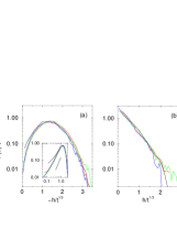
FIG. 3.: Scaled probability distribution $\widetilde{P}(h,t)\cdot t^{1/3}$ for 10 samples of size $L=3000$, with (a) an upper wall [inset: log-log plot; straight line indicates $(|h|/t^{1/3})^{2}$], and (b) a lower wall. The different curves are for $t=500,2500,5000,10000$.

To appreciate the origin of this difference, let us consider the evolution of a piece of flat interface $h=0$ at the critical point $a=a_{c}=a_{0}-a_{1}$. The local drift rate $\langle\partial_{t}h\rangle\approx\langle(\mbox{\boldmath$\nabla$}h)^{2}\rangle-a_{1}$ is negative since $h=0$ and $\mbox{\boldmath$\nabla$}h=0$ there. In the case of a lower wall, this negative drift has no effect since the interface cannot penetrate below the wall. A steady state results from a dynamic balance between the driving force $(a-a_{c}<0)$ which “flattens” pieces of the interface against the wall, and the noise $\eta$ which roughens the interface. Thus, the situation is very similar to the zero-dimensional case, and we expect the exponent results obtained above from the naive scaling analysis to be valid for all $d$.

The situation is very different for the case of an upper wall, since the negative drift represents a significant force repelling the interface from the wall. The effective repulsion exerted by the upper wall is in fact long ranged: Suppose the interface is on average at a distance $\bar{h}$ from the wall. Then interfacial roughness is “interrupted” by the wall at a scale $\bar{\xi}\sim\bar{h}^{2}$ in 1d, leading to an effective repulsive force $\langle\partial_{t}h\rangle\sim-1/\bar{\xi}^{\nu}\sim-1/\bar{h}^{2}$. Thus, a steady state can only be achieved by keeping the interface away from the wall. This necessarily leads to the depletion of $\widetilde{P}(h,t)$ for small $|h|$. In analogy to the problem of a random walker in the vicinity of an absorbing wall, we expect $\widetilde{P}$ to have a power law form, $\widetilde{P}(h,t)\sim(|h|/t^{1/3})^{\sigma}$ for $|h|\ll t^{1/3}$. Our numerical results (Fig. 3(a) inset) are consistent with this power law form, with the exponent $\sigma\approx 2$. The new form of $\widetilde{P}$ for the upper wall allows us to obtain moments of $n$ in terms of the exponent $\sigma$. We find $\theta_{m}=(1+\sigma)\cdot\omega\approx 1$. Our numerical result $\theta_{m}\approx 1.1\pm 0.1$ (Fig. 1(c)) is consistent with this exponent relation. The anomalous exponents can in principle be computed by analyzing the effect of nonlinearity along the line of Ref. [11], but starting with the exact knowledge of the KPZ equation in $d=1$.

Away from the critical point, the form of $\widetilde{P}(h)$ is simply obtained by replacing $\delta h(t)\sim t^{\omega}$ with $|a-a_{c}|^{-\nu(2-z)}=|a-a_{c}|^{-1/2}$ in $d=1$. Our numerics for the lower wall problem (Fig. 3(b)) suggests that $\widetilde{P}(h)\propto\exp\left[-c\,h(a_{c}-a)^{1/2}\right]$ where $c$ is a nonuniversal constant. This exponential distribution of $h$ (which we have also checked directly by numerics) leads to a power law distribution of $n$ as in the zero-dimensional case. Again, we expect this result to be valid for all $d$. For the upper wall problem, the depletion effect described by the extra factor $[|h|(a-a_{c})^{1/2}]^{\sigma}$ in $\widetilde{P}(h)$ leads to logarithmic corrections to the power law form of $P(n)$.

In summary, nonlinear diffusion with multiplicative noise has been analyzed in terms of the dynamic unbinding of an interface from a wall. Two distinct universality classes are obtained for the upper and lower walls in finite spatial dimensions. The upper wall problem, which describes various saturation effects, exhibits anomalous scaling due to nontrivial interaction with the wall. In contrast, the lower wall problem, which models the interaction of a growing interface with a substrate and the fluctuation of wealth in economic systems, can be understood by combining and applying the knowledge of the 0-d problem and the KPZ equation. It is interesting to note that the lower wall problem, in particular the numerical algorithm used here for the hard lower wall, resembles the algorithms used for the “local, gapped” alignment of DNA sequences [16, 17]. (Similarly, the 0-d problem is analogous to gapless local alignment [18].) Divergent critical fluctuations described in this work have a significant effect on the optimization of sequence alignment and will be discussed in detail elsewhere.

We are grateful to M. Lässig, Yuhai Tu, G. Grinstein and A.V. Gruzinov for discussions. M.A.M. acknowledges financial support from the University of Granada and the hospitality of the Physics Department at UC San Diego. T.H. is supported by an A.P. Sloan Research Fellowship and an ONR Young Investigator Award.

REFERENCES

- [1] See, e.g., J.M. Deutsch, Physica A 208, 433 (1994); 445 (1994); and references therein.
- [2] R. A. Fisher, Ann. Eugenics 7, 355 (1937).
- [3] M. Levy and S. Solomon, Int. J. Mod. Phys. C 7, 65 (1996).
- [4] N.G. van Kampen, Stochastic Processes in Physics and Chemistry, (North Holland, 1981).
- [5] M. Kardar, G. Parisi and Y.C. Zhang, Phys. Rev. Lett 56, 889 (1986); E. Medina et al, Phys. Rev. A 39, 3053 (1989).
- [6] J. Krug and H. Spohn in Solids far from equilibrium: Growth, Morphology and Defects, C. Godreche ed. (Cambridge University Press, 1991).
- [7] R. Graham and A. Schenzle, Phys. Rev. A 25, 1731 (1982); A. Schenzle and H. Brand, Phys. Rev. A 20, 1628 (1979).
- [8] M. Levy and S. Solomon, Int. J. Mod. Phys. C 7, 595 (1996); ibid 7, 745 (1996).
- [9] D. Sornette and R. Cont, preprint (1996).
- [10] A.B. Atkinson and A.J. Harrison, Distribution of total wealth in Britain, (Cambridge University Press, 1978).
- [11] Y. Tu, G. Grinstein and M.A. Muñoz, Phys. Rev. Lett. 78, 274, (1997). See also G. Grinstein, M.A. Muñoz and Y. Tu, Phys. Rev. Lett. 76, 4376 (1996).
- [12] Note that the calculation used in [11] to derive the bound for the case cannot be extended to .
- [13] Note that the critical value can be either negative (Stratanovich dynamics) or positive (Ito dynamics). Consequently, a system with may be on either side of the transition depending on the details of the dynamics. Similar dependence may exist and become relevant in the magnetic dynamo problem [14].
- [14] H.K. Moffatt, Magentic field generation in electrically conducting fluids, (Cambridege University Press, 1978).
- [15] P. Grassberger and A. de la Torre, Ann. Phys. (N.Y.) 122, 373 (1979).
- [16] T.F. Smith and M.S. Waterman, J. Mol. Biol. 147, (1981).
- [17] T. Hwa and M. Lässig, Phys. Rev. Lett. 76, 2591 (1996); and to be published.
- [18] S. Karlin and S.F. Altschul, Proc. Natl. Aca. Sci. USA 87, 2264 (1990).