Boundary effects in superfluid films

Abstract

We have studied the superfluid density and the specific heat of the $x-y$ model on lattices $L\times L\times H$ with $L\gg H$ (i.e. on lattices representing a film geometry) using the Cluster Monte Carlo method. In the $H$-direction we applied staggered boundary conditions so that the order parameter on the top and bottom layers is zero, whereas periodic boundary conditions were applied in the $L$-directions. We find that the system exhibits a Kosterlitz-Thouless phase transition at the $H$-dependent temperature $T_{c}^{2D}$ below the critical temperature $T_{\lambda}$ of the bulk system. However, right at the critical temperature the ratio of the areal superfluid density to the critical temperature is $H$-dependent in the range of film thicknesses considered here. We do not find satisfactory finite-size scaling of the superfluid density with respect to $H$ for the sizes of $H$ studied. However, our numerical results can be collapsed onto a single curve by introducing an effective thickness $H_{eff}=H+D$ (where $D$ is a constant) into the corresponding scaling relations. We argue that the effective thickness depends on the type of boundary conditions. Scaling of the specific heat does not require an effective thickness (within error bars) and we find good agreement between the scaling function $f_{1}$ calculated from our Monte Carlo results, $f_{1}$ calculated by renormalization group methods, and the experimentally determined function $f_{1}$.

I Introduction

The theory of second order phase transitions is based on the assumption that at temperatures close to the critical temperature $T_{\lambda}$ there is only one dominating length scale associated with the critical behavior of the system, the correlation length. Since the correlation length diverges as the critical temperature is approached the microscopic details of the system are irrelevant for its critical behavior. This intuitive picture has its foundation in the renormalization group treatment of second order phase transitions. Within the renormalization group treatment it becomes evident that the critical behavior can be divided into different universality classes. Each universality class is characterized by a set of critical exponents which describe the singular behavior of physical quantities in terms of the reduced temperature $t=T/T_{\lambda}-1$, e.g. for a three-dimensional bulk system the correlation length $\xi(t)$ diverges close to $T_{\lambda}$ as $\xi(t)=\xi_{0}^{\pm}|t|^{-\nu}$.

If the system is confined in a finite geometry (e.g. a cubic or film geometry) the singularities in the physical quantities are smoothed out or a crossover to lower-dimensional critical behavior takes place. Finite-size scaling theory [1] is thought to describe well the behavior of the system at temperatures close to $T_{\lambda}$. The intuitive idea behind the finite-size scaling theory is that finite-size effects can be observed when the bulk correlation length becomes of the order of the system size (for a film geometry this is the film thickness $H$). For a physical quantity $O$ this statement can be expressed as follows [2]:

$$\frac{O(t,H)}{O(t,H=\infty)}=f\left(\frac{H}{\xi(t,H=\infty)}\right),$$ (1)

$f$ is a universal function depending only on the geometry and the boundary conditions applied.

Though earlier experiments on superfluid helium films of finite thickness [3] seemed to confirm the validity of the approach outlined above, in a recent experiment Rhee, Gasparini, and Bishop [4, 5] showed that their data for the superfluid density of thick helium films do not satisfy Eq. (1) when the expected value $\nu=0.67$ is used. (For a comprehensive review of experiments on ⁴He to test the finite-size scaling theory cf. Ref.[6].) As an attempt to understand these discrepancies between theory and experiment renormalization group calculations for the standard Landau-Ginzburg free energy functional in different geometries with Dirichlet boundary conditions (vanishing order parameter at the boundary) have been carried out [7, 8, 9, 10, 11]. New specific heat measurements [12] and also a reanalysis [13] of the old specific heat data [14] show good agreement between the renormalization group calculations reported in [7, 8, 9, 10] and those data. These calculations demonstrated the important role played by the boundary conditions. In particular, periodic boundary conditions were shown to be inadequate compared to Dirichlet boundary conditions to describe the experimental specific heat data. The renormalization group calculations have determined the specific heat for that range of the scaling variable where the surface contribution to the specific heat is dominant [8, 9, 10, 15] (c.f. also [16]). Such field theoretical calculations are not available for the case of the superfluid density and the lack of scaling in the case of the superfluid density of helium films is not understood. Furthermore, new experiments on liquid ${}^{4}He$ under microgravity conditions are planned [17] to examine the finite-size scaling properties of the specific heat. In order to test the renormalization group calculations and because of the reasons above, numerical investigations of the finite-size scaling properties of the superfluid density [18] and the specific heat [19, 20] of thin helium films have been carried out. In Refs. [18, 19], we used the $x-y$ model with periodic boundary conditions in the direction of the film thickness $H$ to compute the superfluid density and the specific heat of thin helium films. We demonstrated scaling with respect to the film thickness using the expected values for the critical exponents of the superfluid density and the specific heat, thus confirming the validity of the finite-size scaling theory. However, the obtained universal function for the specific heat does not match the experimentally determined universal function of Ref. [12], indicating that periodic boundary conditions are only a poor approximation of the correct physical boundary conditions as was already demonstrated in Ref.[10]. Later we employed staggered-spin boundary conditions in the top and bottom layers of the film which improves the agreement between the numerically computed scaling function and the experimentally determined scaling function of the specific heat [20].

Another example where the boundary conditions play a role in the scaling behavior comes from Ref. [21] where the Villain model, which also belongs to the $x-y$ universality class, was studied in a film geometry with open boundary conditions in the direction of the film thickness. The authors of Ref. [21] extracted the thickness dependent critical temperature from the temperature dependence of the correlation length in the disordered phase and found for the critical exponent $\nu$ the value $\nu=0.71(1)$ which is different from its value of $0.6705$ known from experiments on liquid Helium[22].

In this paper we intend to study the effect of staggered-spin boundary conditions (Dirichlet–like boundary conditions, i.e. vanishing order parameter on the film boundaries) on the finite-size scaling behavior of the superfluid density and the specific heat of ${}^{4}He$ in a film geometry in detail. Dirichlet–like boundary conditions are believed to approximate the physical boundary conditions more closely [10, 23]. Throughout our numerical calculations we are going to describe superfluid ${}^{4}He$ near the $\lambda$-critical point by another form of the standard Landau-Ginzburg free energy functional: the $x-y$ model (cf. e.g. Ref. [24]). In the pseudospin notation the $x-y$ model takes the following form:

$${\cal H}=-J\sum_{\langle i,j\rangle}\vec{s}_{i}\cdot\vec{s}_{j},$$ (2)

where the summation is over all nearest neighbors, the two-component vector $\vec{s}=(\cos\theta,\sin\theta)$, and $J>0$ sets the energy scale. The angle $\theta$ corresponds to the phase of the expectation value of the helium atom creation operator which is defined in a volume whose linear extensions are much larger than the interparticle spacing and much smaller than the correlation length.

In this article we study the superfluid density which corresponds to the helicity modulus in the pseudospin notation and the specific heat of the $x-y$ model in a film geometry, i.e. on $L^{2}\times H$ lattices with $L\gg H$. The top and bottom layers are coupled to a static staggered spin configuration, playing the role of the “substrate” layers, so that the magnetization in these layers is exactly zero. The crucial difference between these boundary conditions and periodic boundary conditions is that the superfluid density develops a profile in the $H$-direction, whereas it is completely homogeneous for periodic boundary conditions (cf. also the magnetic profile for the Ising model in a film geometry with different boundary conditions in Ref. [25]). We applied periodic boundary conditions in the $L$-directions because we intend to take the limit $L\to\infty$. In the temperature range where the model behaves effectively two-dimensionally we used the Kosterlitz-Thouless-Nelson renormalization group equations to compute the values for the helicity modulus in the $L\rightarrow\infty$ limit. This way we eliminated the $L$-dependence of our data for the helicity modulus and were able to extract the Kosterlitz-Thouless transition temperature $T_{c}^{2D}(H)$ for different films. We investigated the validity of finite-size scaling for the superfluid density and the specific heat of such films of infinite planar dimension and finite $H$. We shall also discuss scaling of the experimental results for the specific heat and superfluid density with respect to the film thickness and compare the universal scaling functions to those obtained from our theoretical investigation.

The rest of this paper is organized as follows. In the next section we introduce the physical observables defined for the $x-y$ model and the numerical method we applied to carry out the calculations. In section III, we discuss the finite-size scaling theory and boundary effects. In section IV we discuss our results and the last section briefly summarizes the work described in this paper.

II Physical observables and Monte Carlo method

For the $x-y$ model on a cubic lattice the helicity modulus is defined as follows [26, 27]:

$$\frac{\Upsilon_{\mu}}{J} = \frac{1}{V}\left\langle\sum_{\langle i,j\rangle}\cos(\theta_{i}-\theta_{j})(\vec{e}_{\mu}\cdot\vec{\epsilon}_{ij})^{2}\right\rangle$$ (4)

$$-\frac{\beta}{V}\left\langle\left(\sum_{\langle i,j\rangle}\sin(\theta_{i}-\theta_{j})\vec{e}_{\mu}\cdot\vec{\epsilon}_{ij}\right)^{2}\right\rangle,$$

where $V$ is the volume of the lattice, $\beta=J/k_{B}T$, $\vec{e}_{\mu}$ is the unit vector in the corresponding bond direction, and $\vec{\epsilon}_{ij}$ is the vector connecting the lattice sites $i$ and $j$. In the following we will omit the vector index since we will always refer to the $x$-component of the helicity modulus. Note that, because of isotropy, we have $\Upsilon_{x}=\Upsilon_{y}$. The connection between the helicity modulus and the superfluid density $\rho_{s}$ is established by the relation [28]

$$\rho_{s}(T)=(\frac{m}{\hbar})^{2}\Upsilon(T),$$ (5)

where $m$ denotes the mass of the helium atom. The specific heat $c$ is obtained from the energy $E$ through

$$c=\frac{\beta^{2}}{N}\left(\langle E^{2}\rangle-\langle E\rangle^{2}\right),$$ (6)

where the energy is defined as:

$$E=\sum_{\langle i,j\rangle}\left(1-\vec{s}_{i}\cdot\vec{s}_{j}\right)$$ (7)

and $N$ is the number of spins contributing to the specific heat.

The thermal averages denoted by the angular brackets are computed according to

$$\langle O\rangle=Z^{-1}\int\prod_{i}d\theta_{i}\>O[\theta]\exp(-\beta E).$$ (8)

$O[\theta]$ denotes the dependence of the physical observable $O$ on the configuration $\{\theta_{i}\}$, the partition function $Z$ is given by

$$Z=\int\prod_{i}d\theta_{i}\>\exp(-\beta E),$$ (9)

The multi-dimensional integrals in the expressions (8) and (9) are computed by means of the Monte Carlo method using Wolffs 1-cluster algorithm [29].

We computed the helicity modulus and the specific heat on $L^{2}\times H$ lattices, where $L=20,40,60,80,100$ and $H=4,8,12,16,20,24$. We applied periodic boundary conditions in the $L$-directions, whereas the first and the $H$-th layer are coupled to a boundary layer which consists of a staggered spin configuration, i.e.

$$\vec{s}(x,y)=(-1)^{x+y}\vec{s}(1,1),$$ (10)

where $x,y\in[1,L]$ and label the integer coordinates of the lattice sites in a plane perpendicular to the $H$-direction. Thus, we have $V=HL^{2}a^{3}$ with $a$ denoting the lattice spacing and $N=HL^{2}$. We carried out of the order of $20,000$ thermalization steps and of the order of $750,000$ measurements. The calculations were performed on a heterogeneous environment of computers including Sun, IBM RS/6000 and DEC alpha AXP workstations and a Cray-YMP.

III Finite-size scaling and boundary effects

A The helicity modulus

Here we shall discuss the finite-size scaling theory of the superfluid density. In Ref. [18], we studied the helicity modulus $\Upsilon$ for the $x-y$ model in a film geometry with periodic boundary conditions in the $H$-direction and we have shown the following steps. In a certain temperature range around the bulk critical temperature $T_{\lambda}$ where the bulk correlation length $\xi(T)$ becomes of the order of the film thickness $H$ the quantity $\Upsilon H/T$ exhibits effectively two-dimensional behavior and a Kosterlitz-Thouless phase transition takes place at a temperature $T_{c}^{2D}(H)<T_{\lambda}$. The critical temperature $T_{c}^{2D}(H)$ approaches $T_{\lambda}$ in the limit $H\rightarrow\infty$ as

$$T_{c}^{2D}(H)=T_{\lambda}\left(1+\frac{x_{c}}{H^{1/\nu}}\right),$$ (11)

where for periodic boundary conditions we found that $x_{c}=-0.9965(9)$ using for the critical exponent $\nu$ the experimental value $\nu=0.6705$ [22] and for $T_{\lambda}$ the value $T_{\lambda}=2.2017$ [30]. The quantity $\Upsilon H/T$ is a function of the ratio $H/\xi(T)$, i.e.

$$\frac{\Upsilon(T,H)H}{T}=\Phi(tH^{1/\nu}).$$ (12)

The universal function $\Phi(x)$ has the properties [31]

$$\Phi(x>x_{c}) = 0,$$ (13)

$$\Phi(x_{c}) = \frac{2}{\pi}.$$ (14)

In the limit $x\rightarrow x_{c}^{-}$ the function $\Phi(x)$ can be written as:

$$\Phi(x)=\frac{2}{\pi}\left(1+A\sqrt{x_{c}-x}\right),$$ (15)

where for periodic boundary condition we found that $A=0.593(5)$. This form of the universal function reconciles the scaling expression (12) with the two-dimensional behavior [32], i.e. as $T\to T_{c}^{2D}(H)$

$$\frac{\Upsilon(T,H)H}{T}=\frac{2}{\pi}\left(1+b(H)\sqrt{1-\frac{T}{T_{c}^{2D}(H)}}\right)$$ (16)

where [33]

$$b(H)=AH^{1/2\nu}.$$ (17)

The results stated above confirm the theoretical expectations about scaling given by Ambegaokar et al. in Ref. [31] and agree with the experimental findings of Bishop and Reppi [34] and Rudnick [35]. In the case of periodic boundary conditions in the $H$-direction the validity of the finite-size scaling form (12) can already be observed for films of thicknesses $H=6,8,10$ [18].

If nonperiodic boundary conditions are introduced Privman argued that the general scaling form (12) has to be altered into [36]

$$\frac{\Upsilon(T,H)H}{T}=\bar{\Phi}(tH^{1/\nu})+\omega\ln H+d,$$ (18)

where $\omega$ and $d$ are constants depending on the boundary conditions. The Monte Carlo data for the helicity modulus obtained from a Monte Carlo simulation of the $x-y$ model on cubes $H\times H\times H$ where the spins in the boundary layers were all parallel (pinned-surface-spin boundary conditions), were found to be consistent with the presence of the logarithmic term in the scaling form (18) [37].

Let us now investigate the consequences of the logarithmic term in (18). Again we have to reconcile the two-dimensional behavior (16) and the general scaling form (18) for temperatures close to the critical temperature $T_{c}^{2D}(H)$ for thick enough films. Introducing the expression (11) for the $H$-dependent critical temperature into Eq. (16) and keeping only terms up to $H^{1/\nu}$ under the square root leads to

$$\frac{\Upsilon(T,H)H}{T}=\frac{2}{\pi}+b(H)H^{-1/2\nu}\sqrt{x_{c}-tH^{1/\nu}}.$$ (19)

where we have absorbed the factor of $2/\pi$ in the definition of $b(H)$. With the assumption (17) we may make the identification

$$\bar{\Phi}(x)=A\sqrt{x_{c}-x}.$$ (20)

In order to account for the logarithmic term in (18) we have to abandon the universal jump at $T_{c}^{2D}(H)$

$$\frac{\Upsilon(T_{c}^{2D}(H),H)H}{T_{c}^{2D}(H)}=\frac{2}{\pi},$$ (21)

instead we have to assume

$$\frac{\Upsilon(T_{c}^{2D}(H),H)H}{T_{c}^{2D}(H)}=d+\omega\ln H,$$ (22)

i.e. the jump becomes $H$-dependent. (The numerical values for $x_{c}$ and $A$ will be different from the values given above as they depend on the boundary conditions.) Eq. (22) means that for nonperiodic boundary conditions in the $H$-direction expression (16) has to be generalized to

$$\frac{\Upsilon(T,H)H}{T}=g(H)+b(H)\sqrt{1-\frac{T}{T_{c}^{2D}(H)}},$$ (23)

where

$$b(H) = AH^{1/2\nu},$$ (24)

$$g(H) = d+\omega\ln H.$$ (25)

B The specific heat

For the finite-size scaling of the specific heat one can use similar scaling expressions to Eq. (1) which were examined in detail in Ref. [18]. The finite-size scaling expression for the specific heat $c$ can also be written in an equivalent way as [7, 8]:

$$\left(c(t,H)-c(t_{0},\infty)\right)H^{-\alpha/\nu}=f_{1}(tH^{1/\nu}).$$ (26)

The function $f_{1}(x)$ is universal and $\nu=0.6705$. At the reduced temperature $t_{0}$ the correlation length is equal to the film thickness $H$, i.e. $t_{0}=(\xi_{0}^{+}/H)^{1/\nu}$ with $\xi_{0}^{+}=0.498$ [38]. This scaling form has been used to analyze the experimental data and, thus, we shall also discuss the scaling of the specific heat using this form in order to compare to published experimental results for the universal function $f_{1}$. We have

$$c(t_{0},\infty)=c(0,\infty)+\tilde{c}^{+}_{1}\left(\frac{\xi_{0}^{+}}{H}\right)^{-\alpha/\nu},$$ (27)

where we have found that $c(0,\infty)=30$, $\tilde{c}_{1}^{+}=-30$ [19] and $\alpha/\nu=-0.0172$ because of the hyperscaling relation $\alpha=2-3\nu$. In Ref. [19] we demonstrated that our numerical results for the specific heat of the $x-y$ model on a film geometry with periodic boundary conditions follow the finite-size scaling form (26) for the thicknesses as small as $H=6,8,10$.

IV Results

Here we shall present our results for the superfluid density and the specific heat and our analysis for the case of staggered-spin boundary conditions as defined in II.

A The helicity modulus

In this section we would like to determine the values of the ratio $\Upsilon(T,H)H/T$ in the limit $L\rightarrow\infty$ and find estimates for the critical temperatures $T_{c}^{2D}(H)$ and the parameters $g(H)$ and $b(H)$ (cf. Eq. (23)). In order to do this we follow closely the procedure described in Refs. [18, 39].

Fig. 1 displays the Monte Carlo data for the helicity modulus in units of the lattice spacing $a$ and the energy scale $J$ for the film of fixed thickness $H=4$. This figure demonstrates that staggered boundary conditions for the top and bottom layers of the film strongly suppress the values of the helicity modulus with respect to the case of periodic boundary conditions. As a consequence films with staggered boundary conditions have a smaller critical temperature than films with periodic boundary conditions.

At the temperature $T=2.1331$ we computed the helicity modulus on a $60\times 60\times 20$ lattice for each layer separately and plotted the result $\Upsilon_{L}(z)/J$ in Fig. 2, where $z$ enumerates the layers. The layered helicity modulus is symmetric with respect to the middle layer where it reaches its maximum and decreases when the boundaries are approached. Although the helicity modulus $\Upsilon(T,H,L)/J$ is not the average of the quantity $\Upsilon_{L}(z)/J$ over all layers (this is due to the second nonlinear term in expression (4)), the curve in Fig. 2 is an approximation to the profile the superfluid density develops in thin films.

Let us turn now to the computation of the values for the ratio $K=T/(\Upsilon H)$ in the $L\rightarrow\infty$ limit. For a fixed thickness $H$ and at temperatures $T$ below but sufficiently close to the critical temperature $T_{c}^{2D}(H)$ the system behaves like a two-dimensional system[31, 18]. In this regime we demonstrated[18] that the dimensionless ratio $K$ obeys the Kosterlitz-Thouless-Nelson renormalization group equations [32, 40, 41]:

$$\frac{dK(T,l)}{dl} = 4\pi^{3}y^{2}(T,l),$$ (28)

$$\frac{dy(T,l)}{dl} = (2-\pi K^{-1}(T,l))y(T,l).$$ (29)

$\ln y$ is the chemical potential to create a single vortex, $e^{l}$ denotes the size of the core radius of a vortex. These equations contain the universal jump $K(T_{c}^{2D}(H),H)=\pi/2$. In order to adjust the above equations to the possibility of an $H$-dependent jump of the ratio $K$ at $T_{c}^{2D}(H)$ we generalize equations (28) and (29) to:

$$\frac{dK(T,l)}{dl} = \zeta y^{2}(T,l),$$ (30)

$$\frac{dy(T,l)}{dl} = 2(1-\epsilon K^{-1}(T,l))y(T,l),$$ (31)

where $\zeta$ and $\epsilon$ are $H$-dependent constants. After eliminating the variable $y$ from the coupled system of differential equations we obtain:

$$\frac{dK(T,l)}{dl}=4(K(T,l)-\epsilon\ln K(T,l)-C),$$ (32)

where $C$ is a constant which satisfies the condition $C\geq\epsilon(1-\ln\epsilon)$. This condition allows for the existence of roots of the right hand side of Eq. (32). If we identify the scale $l$ with $\ln L$ up to a constant we can use Eq. (32) to extrapolate the computed values $K(T,H,L)$ obtained on lattices of finite planar dimension $L$ to the $L=\infty$ limit. Namely, at $L=\infty$ the left hand side of Eq. (32) vanishes [32, 40, 41] and $K(T,H,\infty)<\epsilon$ is given by the root of the right hand side of Eq. (32). The parameters $\epsilon$ and $C$ are found by fitting the Monte Carlo data for $K(T,H,L)$ at a fixed $H$ to the numerical solution to Eq. (32). Table I contains our fitting results for the fitting parameters $\epsilon$ and $C$ and the values for $K(T,H,\infty)$ for the thicknesses $H\in[4,20]$ and Fig. 3 shows a typical fit. We were not able to explore the two-dimensional region for the film with $H=24$ because the temperature range where the film behaves two-dimensional becomes very narrow and our computer resources did not allow an accumulation of data accurate enough to resolve this region.

In Fig. 4 we plot $\Upsilon(T,H)H/T$ versus $tH^{1/\nu}$ for the thicknesses $H=12,16,20,24$ to check the validity of the scaling form (12) where $\nu=0.6705$. The data for the helicity modulus used in Fig. 4 have completely lost their $L$-dependence. We do not obtain a universal scaling curve, thus scaling according to the expression (12) is not valid for the films with thicknesses up to $H=24$. Therefore we will try to employ the scaling form (18) which requires the knowledge of $g(H)$. Since $K^{-1}(T,H,\infty)$ satisfies Eq. (23) for a fixed $H$ and temperatures close enough to the critical temperature $T_{c}^{2D}(H)$ we can fit the obtained results for $K^{-1}(T,H,\infty)$ to Eq. (23) and find an estimate for $T_{c}^{2D}(H)$ and the parameters $b(H)$ and $g(H)$. In Table II we present our fitting results and Fig. 5 shows the fit to the data for $\Upsilon(T,H)H/T$ at $H=4$. It is interesting to note that the $H$-dependence of the parameter $g$ can be described by the formula

$$g(H)=0.338(19)\ln H-0.238(35)$$ (33)

for $H\in[4,20]$. This is consistent with Privman’s prediction [36]. In Fig. 6 we plot $\Upsilon(T,H)H/T-g(H)$ versus $tH^{1/\nu}$ for $H=8,12,16,20$ where $g(H)$ is given in Table II, the bulk critical temperature $T_{\lambda}=2.2017$. Also the scaling form (18) does not collapse our data points onto one universal curve. This situation is the same as the one Rhee, Gasparini and Bishop encountered when they tried to verify finite-size scaling for their data of the superfluid density [4, 5]. Their data of the superfluid density did not fall onto one universal curve when the scaling form (12) was employed, neither did the inclusion of a logarithmic term as in Eq. (18) help to achieve data collapse [5].

Of course, one reason for the failure of scaling of our data of the helicity modulus according to the expressions (12) or (18) could be that our thicknesses are still too small. On the other hand Rhee et al. use films of macroscopic sizes and do not confirm scaling. Furthermore, for films with periodic boundary conditions scaling of the helicity modulus occurs already for thicknesses as small as $H=6$ [18].

Let us therefore pursue another line of thought [42] which we borrow from the mean field treatment of thin ferromagnetic films [43]. The reduced critical temperature of a ferromagnetic film $t_{c}(H)$ ($t_{c}(H)=1-T_{c}^{2D}(H)/T_{c}$ where $T_{c}$ is the 3D bulk critical temperature of the ferromagnet) can be obtained from the following set of equations [43]:

$$u\tan u = \frac{H}{2\lambda},$$ (34)

$$t_{c}(H) = \left(\frac{2a}{H}\right)^{2}u^{2}.$$ (35)

The lattice spacing is denoted by $a$ and $\lambda$ is the extrapolation length $\lambda$ (cf. also Ref. [44]). Let us compute $t_{c}(H)$ in the limit $H/(2\lambda)\gg 1$. From Fig.2 of Ref.[43] it is clear that $u\rightarrow\pi/2$ in the limit $H/(2\lambda)\rightarrow\infty$. Thus, writing $u=\pi/2-\epsilon$ with $0<\epsilon\ll 1$ Eq.(34) turns into

$$\frac{2u\lambda}{H}=\tan\epsilon\approx\epsilon=\frac{\pi}{2}-u.$$ (36)

Solving for $u$ yields

$$u=\frac{\pi}{2\left(1+\frac{2\lambda}{H}\right)}.$$ (37)

Inserting this into Eq.(35) we obtain finally

$$t_{c}(H)=\frac{a^{2}\pi^{2}}{(H+2\lambda)^{2}}.$$ (38)

Thus, within the mean field treatment the reduced critical temperature scales with the correct critical exponent $\nu=0.5$ but with an effective thickness $H+2\lambda$. It is interesting that $2\lambda$ appears in Eq.(38). This means that we have to add twice the extrapolation length (for each side of the film) to the actual thickness. Furthermore, if the magnetization is suppressed close to the boundaries $(\lambda>0)$ the critical temperature $T_{c}^{2D}(H)$ is smaller than the 3D bulk critical temperature and we have to add $2\lambda$ to the actual thickness.

The lack of scaling of our data of the helicity modulus with the expected critical exponent $\nu=0.6705$ indicates that the critical temperatures $T_{c}^{2D}(H)$ do not satisfy Eq. (11). Instead, due to the profile of the superfluid density we may expect an effective film thickness $H_{eff}$ which enters the scaling expressions (11) and (12). In close analogy to the mean field treatment of ferromagnetic films discussed in the paragraph above, we assume that $H_{eff}=H+D$ where $D$ is a constant. Indeed, for the film thicknesses $H=12,16,20$ we obtain $x_{c}=-3.81(14)$ and $D=5.79(50)$ with $\nu=0.6705$. In Fig. 7 we plot $\Upsilon(T,H)H_{eff}/T$ as a function of $tH_{eff}^{1/\nu}$ for films with $H=12,16,20,24$ where $\nu=0.6705$. The data for the helicity modulus collapse reasonably well onto a single curve. We can understand the increment $D$ as a scaling correction which renders the scaling relations (11) and (12) valid even for very thin films. For large thicknesses $H$ the increment $D$ can be neglected and we recover the conventional scaling forms. Of course, it is possible to invent scaling forms different from the structure (38) which yield the conventional scaling expressions in the limit $H\rightarrow\infty$. For example, we have obtained similarly good fitting results using the expression $t_{c}(H)=a_{1}H^{-1/\nu}+a_{2}H^{-2}$ which is also motivated by mean field theory (cf. eg. Ref.[48]). However, since we find Eq.(38) physically appealing we continue to describe the effects of boundary conditions by an effective thickness as we have done in this paragraph.

In order to test further the assumption that the boundaries introduce an effective thickness into the scaling expression (12) we try to describe the thickness dependence of the Kosterlitz-Thouless transition temperature of the Villain model with open boundary conditions (interactions of the top and bottom layer only with the interior film layers) [21] by Eq. (11), where $H$ is replaced by the effective thickness $H_{eff}=H+D_{V}$. Indeed, taking $\nu=0.6705$ we find

$$\left(1-\frac{T_{c}^{2D}(H)}{T_{\lambda}}\right)^{\nu}=\frac{1.384(9)}{H+1.05(2)},$$ (39)

thus $D_{V}=1.05(2)$ and $x_{c}=-1.62(2)$. The function (39) is the solid line in Fig. 8. Again for this case, the increment $D$ is a correction which makes the scaling relations (11) and (12) valid even for very thin films. The result (39) means that the film thicknesses considered in Ref. [21] were still too small to extract the expected value of the critical exponent $\nu$ from the $H$-dependence of the critical temperature (11) without the help of an effective thickness $H+D_{V}$.

In Fig. 9 we achieve approximate collapse of the experimental data of Rhee et al.[4, 5] for the superfluid density $\rho_{s}$ for films of various thickness $d$ ($d$ is in $\mu m$) by plotting $\rho_{s}(t,d)d_{eff}/\rho$ versus $td_{eff}^{1/\nu}$ with $\nu=0.6705$ and $d_{eff}=d+0.145$. This value of the effective thickness was found by examining the reduced temperatures $t_{fs}(H)$ where finite-size effects set in. According to finite-size scaling theory $t_{fs}$ has to fulfill the relation $t_{fs}\propto d^{-1/\nu}$, thus in our case $t_{fs}\propto d_{eff}^{-1/\nu}$. The data corresponding to the film with $d=3.9\mu m$ deviate from the universal curve and we attribute this to the anomalous behavior of these data. Namely, in general $|t_{fs}(d_{1})|>|t_{fs}(d_{2})|$ if $d_{1}<d_{2}$, but this is not the case for $d_{1}=2.8\mu m$ and $d_{2}=3.9\mu m$ (cf. Refs. [4, 5]).

Let us compare the increments over the film thickness for the three cases of film geometry considered above. For the Villain model with open boundary conditions we obtained $D_{V}=1.05(2)$ while for the $x-y$ model with staggered boundary conditions we obtained $D=5.8(5)$. All increments are expressed in lattice spacing units. The difference in these values of the increments reflect how severe the effect of the boundary conditions is. Open boundary conditions are less demanding on the order parameter at the boundary compared to staggered boundary conditions used in our simulations. The value of the increment in the case of ⁴He on silicon is large, $d_{eff}-d=491.5$ in lattice spacing units $a$ ($a=2.95\mbox{\AA}$ [19]). This might cast some doubts on our proposed scaling form for the superfluid data of Rhee et al. It is possible, however, to imagine that on the surface of these films vortices are pinned by impurities or other forms of disorder, which make the order parameter vanish at the boundary and which introduce an effective length scale of such a magnitude.

So far we have seen that different boundary conditions create different effective thicknesses. The influence of the boundaries vanishes for thick enough films and only in a certain small range of film thickness the influence of the boundary conditions has to be taken into account. According to our findings the scaling form (15) for the helicity modulus in the limit $T\to T_{c}^{2D}(H)$ takes the following form now:

$$\frac{\Upsilon(T,H)H_{eff}}{T}=\bar{g}\left(1+A\sqrt{x_{c}-tH_{eff}^{1/\nu}}\right),$$ (40)

where $A$, $x_{c}$ and $\bar{g}$ are constants depending on the boundary conditions. Especially for $tH_{eff}^{1/\nu}=x_{c}$ we should have

$$\frac{\Upsilon(T_{c}^{2D},H)H_{eff}}{T_{c}^{2D}}=\bar{g}.$$ (41)

and this value of $\bar{g}$ is not necessarily equal to $2/\pi$. In Table III we give the values for $\bar{g}$ found by our fitting procedure. We still have a slight $H$-dependence in $\bar{g}$ but for the thicknesses $H\geq 16$ the value for $\bar{g}$ seems to saturate at $\bar{g}(H\to\infty)\approx 0.97$. Since we can neglect the effective thickness for very large film thicknesses, this means that films with staggered boundary conditions in the $H$-direction of the film exhibit a jump in the quantity $\Upsilon(T_{c}^{2D},H)H/T_{c}^{2D}$ that is different from $2/\pi$ which was found for films with periodic boundary conditions [32, 40, 18]. Therefore, assuming that our extrapolation to large film thicknesses from small size films using the idea of the effective thickness is valid, we have to conclude that the jump $\Upsilon(T_{c}^{2D},H)H/T_{c}^{2D}$ depends on the boundary conditions. In principle there is nothing wrong with this conclusion because the universal functions (and the jump is a particular feature of a particular universal function) depend very importantly (especially near the critical temperature) on the boundary conditions. The scaling function should not be confused with the critical exponents which are independent of the geometry and boundary conditions. The scaling functions for given universality, given geometry and boundary conditions are universal. This leads us to the conclusion that this jump in the experimental findings should depend on the substrates (cf. also Ref.[45]). This influence of the substrate must be mediated by the vortices whose generation is enhanced close to the boundaries due to the effect of the boundary (for a more detailed discussion cf. section V). In the experiments the value of $2/\pi$ was found [34, 35], however, the thicknesses of these films are much smaller than the above length scale $D$ found to fit the data of Rhee et al. We believe that the vortex density was almost homogeneous throughout the films used for these measurements. This situation corresponds to the $x-y$ model in a film geometry with periodic boundary conditions along the film direction where the vortex density is the same everywhere.

B The specific heat

In this section we would like to investigate the finite-size behavior of the specific heat $c(T,H)$. Since we do not possess an easily handable procedure to take the $L\rightarrow\infty$ limit for the values of the specific heat $c(T,H,L)$ computed on finite lattices $L\times L\times H$ we approximate films with infinite planar dimension by $100\times 100\times H$ lattices. This seems justified because the specific heat appears independent of $L$ for $L\geq 60$ (cf. Fig. 10). Furthermore, we do not expect the maximum of the specific heat to grow dramatically with increasing values of $L$ because for temperatures in the range $T_{c}^{2D}(H)\leq T\leq T_{\lambda}$ the behavior of the specific heat can be described by the Kosterlitz-Thouless theory which leads to a finite value of this maximum. In order to illustrate this argument we show in Fig. 11 the size dependence of the specific heat $c(T,L)$ computed on pure two-dimensional lattices $L\times L$ with periodic boundary conditions. The $L$-dependence of the specific heat can be neglected for values of $L>80$.

In Fig. 12 we compare the specific heat of films with $H=16,20,24$ to the bulk specific heat $c(t,H=\infty)$ taken from Ref. [19]. The specific heat values for films of thickness $H=12,16,20$ lie above the bulk curve for $t<0$. Such a behavior is also found in experiments on helium films about 30Å thick [6]. This crossing effect is due to the large shift of the temperature $T_{m}$ where the specific heat for a certain film thickness takes its maximum down to temperatures below the bulk critical temperature $T_{\lambda}$. For thicker and thicker films the maximum temperature $T_{m}$ approaches $T_{\lambda}$ , thus the confined specific heat data will fall below the bulk curve which is expected from the field theoretical calculations[8, 9, 10, 46]. The film thicknesses used in our Monte Carlo calculation range from $H=35\mbox{\AA}$ to $H=70.8\mbox{\AA}$ (the lattice spacing $a=2.95\mbox{\AA}$ [19]) which is comparable to the experimental film thicknesses (30Å) where this crossing effect can be observed. Fig. 13 shows the specific heat of the film with $H=24$ alone, indicating that the effect of crossing the bulk curve indeed vanishes for thicker and thicker films. Unfortunately it is beyond our means to carry out the necessary analysis for thicker films than were treated here. It is interesting to note that we find the same qualitative behavior of the specific heat in the case of the $x-y$ model in a cylindrical geometry [47].

In Fig. 14 we plot the scaling function $f_{1}(x)$ given by expression (26). According to the previous discussion this scaling function can only be an approximation to the correct one which one would need to compute from films with $H>24$ and $L>>H$. We find that our data for the specific heat for films of various thicknesses collapse approximately onto a single curve. It seems that the specific heat is rather insensitive to the boundary effect of introducing an effective thickness and a very high accuracy in the computation of the specific heat is needed to detect the presence of the effective thickness in the scaling function $f_{1}(x)$. For example, one could determine the temperatures $T_{m}(H)$ where the specific heat reaches its maximum and examine the validity of Eq. (11) for $T_{m}(H)$, because the $H$-dependence of $T_{m}(H)$ is also given by expression (11) (with a different value for $x_{c}$ than for the critical temperatures $T_{c}^{2D}(H)$). This can be done more easily in experiments because in Monte Carlo calculations an extrapolation procedure for the values of the specific heat at finite planar dimensions to the values at infinite planar dimensions is needed (and which is not available at present) whereas the films used in experiments represent films with infinite planar dimensions.

We can directly compare our function $f_{1}(tH^{1/\nu})$ to the experimentally determined scaling function $f_{1}(x)$ given in Refs. [12] by expressing all lattice units in physical units using the conversion formula:

$$\left.f_{1}(x)\right|_{phys}=\frac{V_{m}k_{B}}{a^{3}}\left(\frac{a}{\mbox{\AA}}\right)^{-\alpha/\nu}\left.f_{1}(x)\right|_{lattice}=15.02\frac{\mbox{Joule}}{{}^{\circ}\mbox{K mole}}\left.f_{1}(x)\right|_{lattice},$$ (42)

where $V_{m}$ is the molar volume of ${}^{4}He$ at saturated vapor pressure at $T_{\lambda}$, the lattice spacing $a=2.95\mbox{\AA}$ [19] and the film thickness is measured in Å. In Fig. 15 we compare the functions $f_{1}(x)$ obtained from Monte Carlo calculations of the specific heat of films with periodic boundary conditions and staggered boundary conditions in the direction of the film thickness to the experimentally determined function $f_{1}(x)$ and to the function $f_{1}(x)$ obtained from field theoretical calculations [8, 9]. This figure clearly shows the influence of the boundary conditions on the shape of the universal function as was already demonstrated by the field theoretical calculations reported in Ref. [10]. In Fig. 15 we see that the scaling function $f_{1}(x)$ for films with staggered boundary conditions crosses the scaling function $f_{1}(x)$ for films with periodic boundary conditions (cf. also [20]) in the range $-14<tH^{1/\nu}<-8$ (cf. Fig. 15) with $H$ measured in Å. This crossing is due to the relative smallness of our film thicknesses (see the discussion above) and does not occur if we had used much thicker films in our Monte Carlo calculations to deduce the scaling function $f_{1}(x)$ [46]. We expect our function $f_{1}(x)$ to be slightly modified in the range $-14<tH^{1/\nu}<-8$ (cf. Fig.15) when it is computed from much thicker films. We believe that the wings of our curve, however, will remain unchanged. Unfortunately, it is beyond our computational means to repeat the calculations for thicknesses larger than 24.

V Discussion of the results

Our findings suggest that it is possible to introduce an effective thickness $H_{eff}=H+D$ into the scaling expressions for the superfluid density (12) and achieve scaling (i.e. data collapse) even for rather thin films. The increment $D$ over the film thickness $H$ can be understood as an effective correction to scaling. The appearance of the effective thickness in our scaling-function can be understood as follows. The superfluid density has a finite value in the first layers next to the boundary layers of the film, and its rise from this finite value to its bulk value $\rho_{s}^{m}(T,H)$ (for $T<T_{C}^{2D}(H)$) inside the film can be divided into two regions. Let us assume that $T$ is very close to $T_{c}^{2D}(H)$ where the correlation length is very large. There is a rather narrow region of thickness $D_{1}$ of the film which is in contact with the boundary wall where the superfluid density rises very fast to attain some value $\rho_{s}^{D_{1}}<\rho_{s}^{m}$. Then it rises with a much slower rate over a length scale of the order of the correlation length to reach its value of $\rho_{s}^{m}$. The reason for the initial fast rise are the correlations over length scales much smaller than the correlation length. One might think that one then has to exclude the region of the film where the superfluid density rises very sharply and this leads to a negative value for $D$. However, this initial rise of $\rho_{s}$ occurs very fast over a length scale $D_{1}$ which is smaller than a length $D_{2}$ which would have been required in order for the superfluid density to reach the same value if this rise would have occurred over larger distances over which the spin-spin correlations are governed by the correlation length which controls the long distance behavior of the correlation function. This implies that the required increment to the thickness is $D=D_{2}-D_{1}$, which is positive.

Only for films with thicknesses $H$ which fulfill $H\gg D$ scaling with $H$ can be observed. For periodic boundary conditions we have $D=0$ [18], open boundary conditions seem to yield $D=1.05$ and for staggered boundary conditions we obtain $D=5.79$. Due to their structure staggered boundary conditions support vortex formation close to the boundaries, thus the superfluid density decreases from its maximum in the middle of the film towards the boundaries. This effect is less pronounced for open and absent for periodic boundary conditions. Our results imply that the more the superfluid density is suppressed near the boundaries the larger is the value of $D$. The data for the superfluid density of Rhee et al. [4] which correspond to ${}^{4}He$ on Si require a large value of $D=0.145\mu m$. Thus, Si should suppress the superfluid density dramatically close to the boundary. Since $D$ is so large, only films with $H>3\mu m$ should allow scaling with $H$. It would be interesting to investigate the scaling behavior of the superfluid density of ${}^{4}He$ on different substrates (which represent different types of boundary conditions) in a wide range of film thicknesses to check our hypothesis.

A consequence of scaling our data of the helicity modulus (or superfluid density) using an effective thickness is that the jump in the quantity $\Upsilon(T_{c}^{2D},H)H/T_{c}^{2D}$ depends on the boundary conditions in the top and bottom layers of the film, i.e. on the substrates in real helium experiments. The value of the jump is only $2/\pi$ (in lattice units) for film thicknesses small compared to $D$ as is the case in the experiments reported in Refs. [34, 35]. The same value of the jump was found is the case for $x-y$ films with periodic boundary conditions [18]. Thus, experiments could be also used to determine the jump in the areal superfluid density at the Kosterlitz-Thouless temperature and determine its substrate dependence.

In this work we represented the substrate by a staggered spin configuration coupled to the top and bottom layers of the film to simulate Dirichlet-like boundary conditions (zero order parameter in the boundary) in the substrate. For the staggered spin configuration the local magnetization is exactly zero on a plaquette, i.e. on a domain of the size $a\times a$ where $a$ denotes the lattice spacing. Dirichlet-like boundary conditions in the substrate are, however, also realized by the following spin configuration: The spins are parallel in a square domain of linear dimension $R$, but any two spins representing two adjacent domains are antiparallel to each other. Thus, an additional length scale associated with a finite value of the local magnetization over the length scale $R$ is introduced and influences the scaling behavior of the helicity modulus and the specific heat. Since disorder in the boundaries supports vortex formation close to the boundaries, vortices should play an active role in creating the boundary effect described above.

VI Summary

We have investigated the finite-size scaling properties of the specific heat $c$ and the helicity modulus $\Upsilon$ of the $x-y$ model in a film geometry, i.e. on $L\times L\times H$ lattices with $L\gg H$ where staggered and periodic boundary conditions where applied in the $H$-direction and the $L$-directions of the film, respectively. We found that a Kosterlitz-Thouless phase transition takes place at the $H$-dependent critical temperatures $T_{c}^{2D}(H)$, however, for the films used in our calculations the jump $\Upsilon(T_{c}^{2D}(H),H)H/T_{c}^{2D}(H)$ appears to be $H$-dependent. Furthermore, scaling of the helicity modulus according to Eq. (12) is not valid for our film thicknesses, neither is scaling according to Eq. (18) which was derived following a suggestion of Privman [36]. Introducing an effective thickness $H_{eff}>H$ into the scaling expression (12) we are able to collapse our data as well as the data of Rhee et al. [4] reasonably well onto one universal curve. Our results suggest that the boundary effect of creating an effective thickness $H_{eff}$ depends on the boundary conditions which can be realized in experiments by different substrates and is negligible for thicknesses $H$ which fulfill $H_{eff}/H-1\ll 1$. We argue that the jump in the quantity $\Upsilon(T_{c}^{2D},H)H/T_{c}^{2D}$ depends on the boundary conditions and is $2/\pi$ only for certain ideal boundary conditions such as the periodic boundary conditions. Within error bars scaling of the specific heat does not require an effective thickness and the scaling function $f_{1}(x)$ for the specific heat agrees rather well with the experimentally determined scaling function $f_{1}(x)$ and with the result of the renormalization group calculations reported in [8, 9]. However, we found that Monte Carlo simulations of much thicker films than we have used have to be performed to determine the position of the maximum of the scaling function accurately. At present this is unfortunately beyond our computer resources.

VII Acknowledgements

We would like to thank Prof. Dohm for interesting and useful discussions. N. S. would like to thank the Höchsleistungsrechenzentrum Jülich for the opportunity of using their computing facilities. This work was supported by the National Aeronautics and Space Administration under grant no. NAG3-1841 and by Sonderforschungsbereich 341 der Deutschen Forschungsgemeinschaft.

FIG. 1.: The helicity modulus $\Upsilon(T,H,L)$ as a function of $T$ for various lattices $L^{2}\times 4$ with staggered boundary conditions (sbc) and periodic boundary conditions (pbc) in the $H$-direction.

FIG. 2.: The approximate profile $\Upsilon_{L}(z)$ of the helicity modulus computed on a $60\times 60\times 20$ lattice at $T=2.1331$, i.e. close to the critical temperature, $T_{c}^{2D}(20)=2.1346$.

FIG. 3.: $T/(\Upsilon(T,H,L)H)$ as a function of $\ln L$ at $T=1.8182$ and $H=4$. The solid curve is the fit to the solution to (32).

FIG. 4.: $\Upsilon(T,H)H/T$ as a function of $tH^{1/\nu}$ for various thicknesses. $\nu=0.6705$.

FIG. 5.: $\Upsilon(T,H)H/T$ at $L=\infty$ and $H=4$ as a function of $T$. The solid curve is the fit to (23).

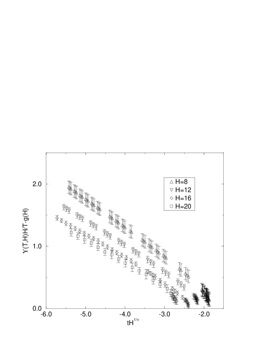
FIG. 6.: $\Upsilon(T,H)H/T-g(H)$ as a function of $tH^{1/\nu}$. $\nu=0.6705$ and the values for $g(H)$ are taken from Table II.

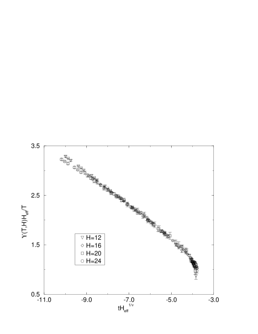
FIG. 7.: $\Upsilon(T,H)H_{eff}/T$ as a function of $tH_{eff}^{1/\nu}$ for various thicknesses. $H_{eff}=H+5.79$ and $\nu=0.6705$.

FIG. 8.: $(1-T_{c}^{2D}(H)/T_{\lambda})^{\nu}$ for the Villain model in a film geometry with open boundary conditions as a function of $H$. The solid line is the expression (39).

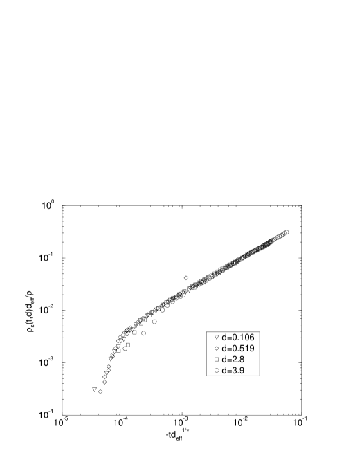
FIG. 9.: Scaling of the superfluid density data of Rhee et al. [4] with the effective thickness $d_{eff}=d+0.145$. $\nu=0.6705$ and all lengths are in $\mu m$.

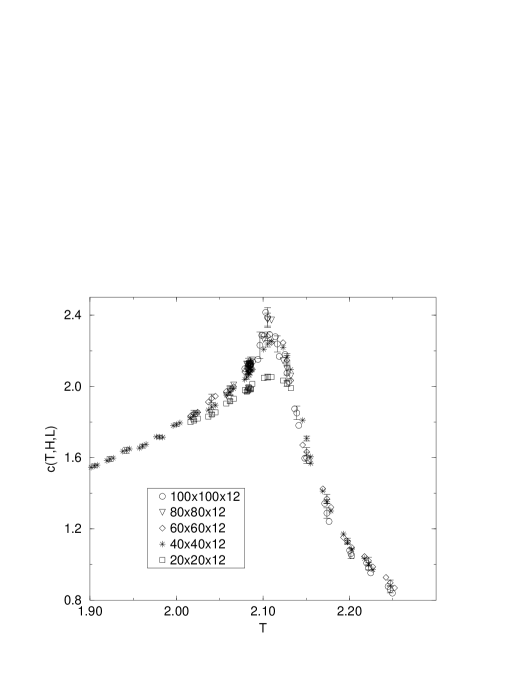
FIG. 10.: The specific heat $c(T,H,L)$ as a function of $T$ for $L^{2}\times 12$ lattices. $T_{c}^{2D}(12)=2.086$, $T_{\lambda}=2.2017$.

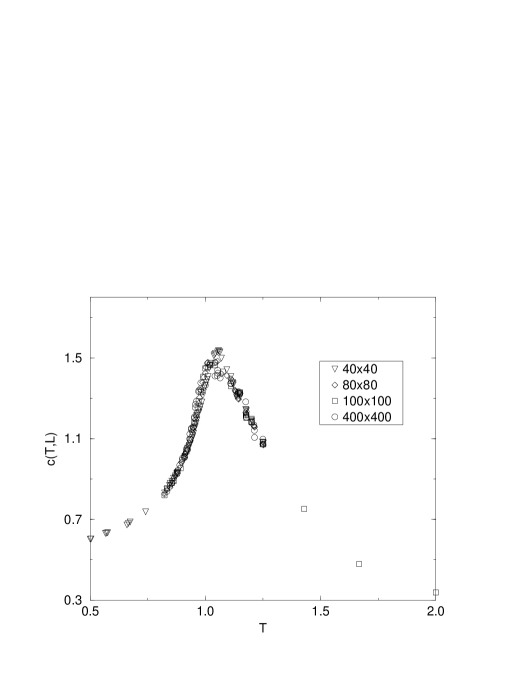
FIG. 11.: The specific heat $c(T,L)$ for pure two-dimensional lattices $L\times L$ with periodic boundary conditions.

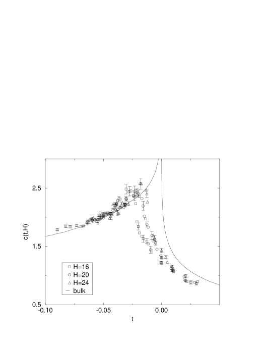
FIG. 12.: The specific heat $c(t,H)$ for various films of finite thickness $H$ compared to the bulk specific heat $c(t,\infty)$.

FIG. 13.: The specific heat $c(t,H)$ for the film of thickness $H=24$ compared to the bulk specific heat $c(t,\infty)$.

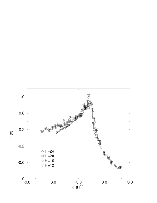
FIG. 14.: Scaling function $f_{1}(x)$ for films with staggered boundary conditions where $x=tH^{1/\nu}$.

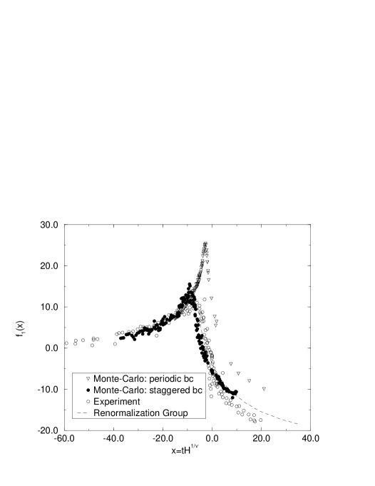
FIG. 15.: The experimentally determined function $f_{1}(x)$ (open circles) of Refs. [12], $f_{1}(x)$ for films with periodic boundary conditions (triangles) of Ref. [19] and staggered boundary conditions (filled circles), and $f_{1}(x)$ for films with Dirichlet boundary conditions of Ref. [8] (dashed line).

$H$	$T$	$\epsilon$	$C$	$K(T,H,\infty)$	$\chi^{2}$	$Q$
4	1.8315	3.2080(6)	-0.51(1)	2.852(87)	0.74	0.39
	1.8305	3.2251(4)	-0.511(9)	2.742(50)	0.16	0.69
	1.8298	3.2222(5)	-0.495(9)	2.674(43)	0.17	0.68
	1.8290	3.2125(5)	-0.470(9)	2.601(37)	0.15	0.70
	1.8265	3.0255(7)	-0.262(7)	2.453(29)	0.58	0.45
	1.8248	3.0353(8)	-0.243(7)	2.347(23)	0.45	0.50
	1.8198	3.1442(6)	-0.244(6)	2.122(12)	0.02	0.89
	1.8182	3.0890(7)	-0.186(3)	2.0866(72)	0.66	0.52
	1.8149	3.5845(1)	-0.478(8)	1.9916(9)	0.03	0.86
	1.8116	5.21092(2)	-1.46(1)	1.9094(7)	0.009	0.92
	1.8083	10.53880(4)	-4.60(4)	1.8434(8)	0.06	0.81
8	2.0167	2.0420(2)	0.624(3)	1.666(14)	1.76	0.18
	2.0161	2.0787(2)	0.614(3)	1.633(12)	1.63	0.20
	2.0155	2.1046(2)	0.608(3)	1.608(11)	1.58	0.21
	2.0147	2.0465(1)	0.641(2)	1.5890(84)	0.16	0.69
	2.0141	2.0371(1)	0.650(2)	1.5750(82)	0.12	0.73
	2.0135	2.0262(1)	0.659(2)	1.5610(83)	0.07	0.79
	2.0127	2.41711(9)	0.509(3)	1.5190(57)	3.12	0.08
	2.0121	2.50265(9)	0.483(4)	1.5032(53)	3.20	0.07
	2.0115	2.53788(9)	0.477(4)	1.4908(57)	3.08	0.08
	2.0107	4.78735(2)	-0.383(9)	1.4739(42)	1.56	0.21
	2.0101	5.54710(2)	-0.65(1)	1.4629(42)	1.48	0.22
	2.0094	3.39908(6)	0.183(6)	1.4528(45)	1.44	0.23
12	2.0846	1.7021(3)	0.818(3)	1.446(14)	1.17	0.28
	2.0842	1.7190(2)	0.817(3)	1.420(12)	0.77	0.38
	2.0838	1.7148(3)	0.822(3)	1.406(12)	0.52	0.47
	2.0833	1.7221(1)	0.822(2)	1.3949(86)	0.25	0.78
	2.0829	1.7664(2)	0.817(2)	1.3582(64)	1.34	0.26
	2.0825	1.7455(2)	0.826(2)	1.3500(66)	1.32	0.27
	2.0822	1.7343(2)	0.831(2)	1.3466(68)	1.29	0.28
	2.0818	2.1259(1)	0.733(3)	1.3140(48)	0.004	0.95
	2.0812	2.1171(1)	0.745(3)	1.2998(47)	0.007	0.93
	2.0805	2.1161(1)	0.754(3)	1.2859(49)	0.06	0.81
16	2.1173	1.4971(3)	0.903(3)	1.327(21)	1.36	0.24
	2.1171	1.5517(3)	0.894(3)	1.294(14)	1.56	0.21
	2.1169	1.5591(3)	0.895(3)	1.282(13)	1.53	0.22
	2.1164	1.5589(3)	0.904(3)	1.241(12)	0.14	0.87
	2.1160	1.7307(2)	0.880(3)	1.2104(61)	1.64	0.19
	2.1153	2.0342(4)	0.842(3)	1.1825(48)	1.05	0.35
	2.1148	1.7092(3)	0.896(2)	1.1816(56)	2.20	0.11
	2.1142	1.5761(3)	0.921(2)	1.1748(68)	0.40	0.67
	2.1119	1.6254(5)	0.936(4)	1.1197(78)	0.42	0.66
20	2.1336	1.280(1)	0.972(2)	1.146(18)	0.32	0.73
	2.1331	1.273(2)	0.974(2)	1.130(16)	0.45	0.64
	2.1327	1.273(3)	0.977(2)	1.109(14)	0.55	0.58
	2.1322	1.238(2)	0.981(2)	1.111(17)	0.13	0.88
	2.1317	1.310(3)	0.982(2)	1.066(10)	0.05	0.95
	2.1313	1.303(2)	0.986(2)	1.0535(94)	0.04	0.96
	2.1308	1.293(1)	0.989(2)	1.0428(91)	0.06	0.94
	2.1299	1.692(2)	1.00(1)	1.001(14)	0.03	0.86

TABLE I.: Fitted values of the parameters $\epsilon$ and $C$ of the expression (32) and the extrapolated values $K(T,H,\infty)$ at various temperatures $T$ and different thicknesses $H$. $\chi^{2}$ and the goodness of the fit $Q$ are also given.

$H$	$g(H)=\Upsilon(T_{c}^{2D}(H),H)H/T_{c}^{2D}(H)$	$b(H)$	$T_{c}^{2D}(H)$	$\chi^{2}$	$Q$
4	0.231(13)	2.564(63)	1.8354(9)	1.15	0.33
8	0.47(10)	2.94(83)	2.0207(41)	0.88	0.54
12	0.587(44)	3.68(57)	2.0862(10)	1.32	0.24
16	0.715(32)	4.07(78)	2.1175(3)	0.23	0.87
20	0.754(53)	4.91(91)	2.1346(7)	0.73	0.60

TABLE II.: Fitted values of the parameters $g(H)$, $b(H)$ and $T_{c}^{2D}(H)$ of the expression (23) for different thicknesses $H$. $\chi^{2}$ and the goodness of the fit $Q$ are also given.

$H$	$\bar{g}=\Upsilon(T_{c}^{2D}(H),H)H_{eff}/T_{c}^{2D}(H)$
4	0.565(32)
8	0.81(17)
12	0.870(65)
16	0.974(44)
20	0.972(68)

TABLE III.: The jump $\bar{g}=\Upsilon(T_{c}^{2D}(H),H)H_{eff}/T_{c}^{2D}(H)$ for different thicknesses $H$.

REFERENCES

- [1] M. E. Fisher and M. N. Barber, Phys. Rev. Lett. 28, 1516 (1972); M. E. Fisher, Rev. Mod. Phys. 46, 597 (1974); V. Privman, Finite Size Scaling and Numerical Simulation of Statistical systems, Singapore: World Scientific 1990.
- [2] E. Brezin, J. Physique 43, 15 (1982).
- [3] J. Maps and R. B. Hallock, Phys. Rev. Lett 47, 1533 (1981).
- [4] I. Rhee, F. M. Gasparini, and D. J. Bishop, Phys. Rev. Lett. 63, 410 (1989).
- [5] I. Rhee, D. J. Bishop, and F. M. Gasparini, Physica B165&166, 535 (1990).
- [6] F. M. Gasparini and I. Rhee, Prog. Low Temp. Phys. XIII, 1 (1992).
- [7] R. Schmolke, A. Wacker, V. Dohm, and D. Frank, Physica B165 & 166, 575 (1990).
- [8] V. Dohm, Physica Scripta T49 46 (1993).
- [9] P. Sutter and V. Dohm, Physica B194-196, 613 (1994).
- [10] W. Huhn and V. Dohm, Phys. Rev. Lett. 61, 1368 (1988).
- [11] M. Krech and S. Dietrich, Phys. Rev. A46 1886 (1992), 1922 (1992).
- [12] J. A. Nissen, T. C. P. Chui, and J. A. Lipa, J. Low Temp. Phys. 92, 353 (1993), Physica B194-196, 615 (1994).
- [13] A. Wacker and V. Dohm, Physica B194-196 611 (1994).
- [14] T. Chen and F. M. Gasparini, Phys. Rev. Lett. 40, 331 (1978); F. M. Gasparini, T. Chen, and B. Bhattacharyya, Phys. Rev. 23, 5797 (1981).
- [15] M. Pitz, Diploma thesis, RWTH Aachen, Germany (1996).
- [16] M. Coleman and J. A. Lipa, Czech. J. Phys. 46 (Suppl. S1), 183 (1996).
- [17] J. A. Lipa, private communications.
- [18] N. Schultka and E. Manousakis, Phys. Rev. B51, 11712 (1995).
- [19] N. Schultka and E. Manousakis, Phys. Rev. B52, 7528 (1995).
- [20] N. Schultka and E. Manousakis, Phys. Rev. Lett. 75, 2710 (1995).
- [21] W. Janke and K. Nather, Phys. Rev. B48 15807 (1993).
- [22] L. S. Goldner and G. Ahlers, Phys. Rev. B45, 13129 (1992).
- [23] V. L. Ginzburg and L. P. Pitaevskii, Soviet Physics, J. E. T. P., 34, 858 (1958). V. L. Ginzburg, Soviet Physics, J. E. T. P. 2, 170 (1956).
- [24] H. Kleinert, Gauge Fields in Condensed Matter, Singapore: World Scientific 1989.
- [25] S. Dasgupta, D. Stauffer, and V. Dohm, Physica A213, 368 (1995).
- [26] S. Teitel and C. Jayaprakash, Phys. Rev. B27, 598 (1983).
- [27] Y.-H. Li and S. Teitel, Phys. Rev. B40, 9122 (1989).
- [28] M. E. Fisher, M. N. Barber and D. Jasnov, Phys. Rev. B16, 2032 (1977).
- [29] U. Wolff, Phys. Rev. Lett. 62, 361 (1989).
- [30] W. Janke, Phys. Lett. A148, 306 (1992).
- [31] V. Ambegaokar, B. I. Halperin, D. R. Nelson and E. D. Siggia, Phys. Rev. B21 1806 (1980).
- [32] D. R. Nelson and J. M. Kosterlitz, Phys. Rev. Lett. 39, 1201 (1977).
- [33] R. G. Petschek, Phys. Rev. Lett. 57, 501 (1986).
- [34] D. J. Bishop and J. D. Reppy, Phys. Rev. Lett. 40, 1727 (1978).
- [35] I. Rudnick, Phys. Rev. Lett. 40, 1454 (1978).
- [36] V. Privman, J. Phys. A23, L711 (1990).
- [37] K. K. Mon, Phys. Rev. B44, 2643 (1991).
- [38] A. P. Gottlob and M. Hasenbusch, Physica A201, 593 (1993).
- [39] N. Schultka and E. Manousakis, Phys. Rev. B49, 12071 (1994).
- [40] J. V. Jose, L. P. Kadanoff, S. Kirkpatrick, and D. R. Nelson, Phys. Rev. B16, 1217 (1977)
- [41] J. M. Kosterlitz, J. Phys. C7, 1046 (1974); J. M. Kosterlitz and D. J. Thouless, J. Phys. C6, 1181 (1973).
- [42] N. Schultka and E. Manousakis, J. Low Temp. Phys. 105, 3 (1996).
- [43] M. I. Kaganov and A. N. Omel’yanchuk, Sov. Phys. JETP 34, 895 (1972).
- [44] K. Binder and P. C. Hohenberg, Phys. Rev. B 6, 3461 (1972).
- [45] N. Schultka and E. Manousakis, Czech. J. Phys. 46 (Suppl. S1), 451 (1996).
- [46] V. Dohm, private communication.
- [47] N. Schultka and E. Manousakis, in preparation.
- [48] J. Rudnick and G. Gaspari, Phys. Rev. B32, 7594 (1985).