Cotunneling at resonance for the single-electron transistor

Abstract

We study electron transport through a small metallic island in the perturbative regime. Using a recently developed diagrammatic technique, we calculate the occupation of the island as well as the conductance through the transistor in forth order in the tunneling matrix elements, a process referred to as cotunneling. Our formulation does not require the introduction of a cut-off. At resonance we find significant modifications of previous theories and good agreement with recent experiments.

Electron transport through small metallic islands is strongly influenced by the charging energy associated with low capacitance of the junctions [1, 2, 3]. A variety of single-electron effects, including Coulomb blockade phenomena and gate-voltage dependent oscillations of the conductance, have been observed. Usually, they are described within the “orthodox theory”[1] which treats tunneling in lowest order perturbation theory (golden rule) and corresponds to the classical picture of incoherent tunneling processes (sequential tunneling). As a necessary condition one needs weak tunneling, i.e., the conductance of the barriers has to be low

$$\alpha_{0}\equiv h/(4\pi^{2}e^{2}R_{\rm T})\ll 1.$$ (1)

Despite the success of this straightforward approach, it was found experimentally and theoretically that there are several regimes where higher order tunneling processes have to be taken into account.

First, in the Coulomb blockade regime, sequential tunneling is exponentially suppressed. The leading contribution to the current is a second-order process in which electrons tunnel via a virtual state of the island. Averin and Nazarov [4] evaluated the transition rate of this “inelastic cotunneling” process at zero temperature. At finite temperature, divergences arise, but the authors of Ref. [4] provide an approximation which is valid far away from the resonances. They assumed that some regularization procedure will overcome the divergences. Their results were confirmed experimentally [5].

Second, it was found recently [6, 7] that even at resonance, where sequential tunneling is not suppressed, higher order processes are important and can lead to a significant change of the conductance. Similar effects were discussed for the average charge of the single-electron box in equilibrium [8, 9, 10, 11, 15]. A diagrammatic real-time technique was developed for metallic islands [6, 7] as well as for quantum dots [12, 13] in order to give a systematic description of the various tunneling processes. The effects from quantum fluctuations were shown to become observable either for strong tunneling $\alpha_{0}\sim 1$ or at low enough temperatures $\alpha_{0}\ln{E_{\rm C}/T}\sim 1$, where $E_{\rm C}$ denotes the charging energy. The predicted broadening of the conductance peak as well as the reduction of its height was confirmed in the experiments of Joyez et al. [14] in the strong tunneling regime. Within the theory, only processes where the two classically occupied charge states are involved (even virtually) were included. Therefore, it was necessary to introduce a band-width cut-off $\sim E_{\rm C}$, which prohibits a comparison with experiment without fitting parameters. However, at low temperatures, a quantitative fit between theory and experiment is possible provided a renormalized value for the charging energy is used as it was determined in the experiment.

In this Letter, we use the same diagrammatic technique to obtain the total current in second order in $\alpha_{0}$ including all relevant processes such that no cut-off remains. All terms are regularized in a natural way. This is important for a comparison with experiments since only system parameters enter the result, while a cut-off or some arbitrary regularization scheme would be an undetermined ingredient in the theory. At resonance we obtain new contributions compared to the existing theory of electron cotunneling. They emerge from a change of the occupation probabilities and a renormalization of the charge excitation energy. For realistic parameters $T/E_{\rm C}\sim 0.05$ and $\alpha_{0}^{\rm L}=\alpha_{0}^{\rm R}\sim 0.02$ the corrections are of order $20\%$. We compare with recent experiments [14] and find reasonable agreement without fitting any parameter.

The single-electron transistor is modeled by the standard tunneling Hamiltonian

$$H=H_{\rm L}+H_{\rm R}+H_{\rm I}+H_{\rm ch}+H_{\rm T}=H_{0}+H_{\rm T}.$$ (2)

Here $H_{\rm r}=\sum_{kn}\epsilon^{\rm r}_{kn}a^{\dagger}_{{\rm r}kn}a_{{\rm r}kn}$ and $H_{\rm I}=\sum_{qn}\epsilon_{qn}c^{\dagger}_{qn}c_{qn}$ describe the noninteracting electrons in the two leads r=L,R and on the island where $n$ is the transverse channel index which includes the spin. The wave vectors $k$ and $q$ numerate the states of the electrons for fixed r and $n$. In the following, we consider “wide” metallic junctions with $N\gg 1$ transverse channels. The Coulomb interaction of the electrons on the island is modeled by $H_{\rm ch}=E_{\rm C}(\hat{n}-n_{\rm x})^{2}$, where $E_{\rm C}={e^{2}\over 2C}$ is the charging energy, and $en_{\rm x}=C_{\rm L}V_{\rm L}+C_{\rm R}V_{\rm R}+C_{\rm g}V_{\rm g}$, with $C=C_{\rm L}+C_{\rm R}+C_{\rm g}$, describes an external charge, which depends on the voltages and capacitances of the circuit. The excess particle number operator on the island is given by $\hat{n}$. The charge transfer processes due to tunneling are described by

$$H_{\rm T}=\sum_{\rm r=L,R}\sum_{kqn}(T^{{\rm r}n}_{kq}a^{\dagger}_{{\rm r}kn}c_{qn}e^{-i\hat{\varphi}}+h.c.)$$ (3)

where $T^{{\rm r}n}_{kq}$ are the tunneling matrix elements and $e^{\pm i\hat{\varphi}}$ changes the excess particle number on the island by $\pm 1$. The tunneling matrix elements $T^{{\rm r}n}_{kq}=T^{{\rm r}n}$ are considered independent of the states $k$ and $q$. They are related to the tunneling resistances $R_{\rm T,r}$ of the left and right junction via ${1\over R_{\rm T,r}}={2\pi e^{2}\over\hbar}\sum_{n}N^{n}_{\rm r}(0)N^{n}_{I}(0)|T^{{\rm r}n}|^{2}$, where $N^{n}_{\rm I}(0)$ and $N^{n}_{\rm r}(0)$ are the density of states of the island and the leads.

In the following we use the diagrammatic technique developed in Ref. [6, 7]. The nonequilibrium time evolution of the charge degrees of freedom on the island is described by its reduced density matrix, which we obtain in an expansion in $H_{\rm T}$. The reservoirs are assumed to remain in thermal equilibrium (with electro-chemical potential $\mu_{\rm r}$) and are traced out by using Wick’s theorem, such that the Fermion operators are contracted in pairs. For a large number of transverse channels $N$, only those configurations contribute where the operators $a^{\dagger}_{{\rm r}kn}c_{qn}$ at one time, i.e., from one term $H_{\rm T}$ are contracted with the operators $c^{\dagger}_{qn}a_{{\rm r}kn}$ from one other term $H_{\rm T}$, and not from different ones. These “simple loops” dominate over more complicated configurations with more than two times connected by contractions. Matrix elements of the reduced density operator are visualized in Fig. (1). The forward and the backward propagator (Keldysh contour) are coupled by “tunneling lines” (simple loops) associated with the junctions to the reservoirs r. Each tunneling line with energy $\omega$ represents the rate $\alpha^{\pm}_{\rm r}(\omega)$ if the line is directed backward (forward) with respect to the closed time path with

$$\alpha^{\pm}_{\rm r}(\omega)=\pm\alpha_{0}^{\rm r}{\omega-\mu_{\rm r}\over\exp[\pm\beta(\omega-\mu_{\rm r})]-1}\,.$$ (4)

They are associated with changes of the charge state, as indicated on the closed time path. Finally, we associate with each tunneling vertex at time $t$ a factor $\exp{(i\Delta E\,t)}$ where $\Delta E$ is the difference of out- and incoming energies. If the vertex lies on the backward propagator it acquires a factor $-1$. We define $\alpha_{0}=\sum_{\rm r}\alpha_{0}^{\rm r}$ and $\alpha(\omega)=\sum_{\rm r}\alpha_{\rm r}(\omega)$.

The transport properties are affected by the energy difference of adjacent charge states

$$\Delta_{n}=E_{\rm ch}(n+1)-E_{\rm ch}(n)=E_{\rm C}[1+2(n-n_{\rm x})]\,.$$ (5)

The formally exact Master equation reads in the stationary case [6, 7]

$$\dot{p}_{n}=\sum\limits_{n^{\prime}\neq n}\left[p_{n^{\prime}}\Sigma_{n^{\prime},n}-p_{n}\Sigma_{n,n^{\prime}}\right]=0$$ (6)

with the probability $p_{n}$ to be in charge state $n$ and transition rates $\Sigma_{n,n^{\prime}}$ to change from state $n$ to $n^{\prime}$. In the perturbative regime we write $p_{n}=p_{n}^{(0)}+p_{n}^{(1)}+p_{n}^{(2)}+\ldots$ and $\Sigma_{n,n^{\prime}}=\Sigma_{n,n^{\prime}}^{(1)}+\Sigma_{n,n^{\prime}}^{(2)}+\Sigma_{n,n^{\prime}}^{(3)}+\ldots$ where $p_{n}^{(k)}$ and $\Sigma_{n,n^{\prime}}^{(k)}$ denotes the term $\sim\alpha_{0}^{k}$ of the expansion. The Master equation must hold in each order. In lowest order (sequential tunneling) it reads $p_{n}^{(0)}\alpha^{+}(\Delta_{n})-p_{n+1}^{(0)}\alpha^{-}(\Delta_{n})=0.$ At low temperature at most two charge states ($n=0,1$) are important, all other states are suppressed exponentially.

Due to higher order processes, however, the occupation is modified and also the probability for the other charge states can be nonzero (they are algebraically suppressed, but not exponentially). The Master equation expanded in second order gives a relation between the rates in second order $\Sigma_{n,n^{\prime}}$ (diagrams with two lines) and the occupation in first order $p_{n}^{(1)}$ which lead to a deviation in the average occupation $\langle n\rangle=\sum_{n}np_{n}=\langle n\rangle^{(0)}+\langle n\rangle^{(1)}+\ldots$.

The stationary current $I_{\rm r}=-ie\sum_{n,n^{\prime}}p_{n}\Sigma_{n,n^{\prime}}^{\rm r+}$ through reservoir $r$ uses the rates $\Sigma_{n,n^{\prime}}^{\rm r+}$ where the rightmost tunneling line corresponds to reservoir r and is an outgoing (incoming) one if the rightmost vertex lies on the upper (lower) propagator (and vice versa for $\Sigma_{n,n^{\prime}}^{\rm r-}$). There are two types of diagrams contributing to the second order correction of the current $I^{(2)}$: those of the form $p^{(0)}\Sigma^{(2)}$ and the others like $p^{(1)}\Sigma^{(1)}$. The first ones correspond to “new”, second order processes, and the second ones are responsible for a modification of the first order processes due to the fact, that the occupation probabilities are changed in higher orders. The latter have not been considered in previous theories. As we will see later, both contributions are important.

In lowest order the average occupation

$$\langle n\rangle^{(0)}=\alpha^{+}(\Delta_{0})/\alpha(\Delta_{0})$$ (7)

is only smeared by temperature. Quantum fluctuations, however, yield

$$\langle n\rangle^{(1)}=-{1\over 2E_{\rm C}}{\partial\over\partial n_{\rm x}}\left[p_{0}^{(0)}\left({\rm Re}\,\sigma^{-}(\Delta_{-1})-{\rm Re}\,\sigma^{+}(\Delta_{0})\right)\right.$$ (8)

$$\left.+p_{1}^{(0)}\left({\rm Re}\,\sigma^{-}(\Delta_{0})-{\rm Re}\,\sigma^{+}(\Delta_{1})\right)\right]$$ (9)

where ${\rm Re}\,\sigma^{\pm}(\omega)=\sum_{\rm r=L,R}{\rm Re}\,\sigma^{\pm}_{\rm r}(\omega)$ and

$${\rm Re}\,\sigma^{\pm}_{\rm r}(\omega)={\rm Re}\,\int\limits_{-\infty}^{\infty}d\omega^{\prime}{\alpha^{\pm}_{\rm r}(\omega^{\prime})\over\omega-\omega^{\prime}+i0^{+}}=$$ (10)

$$\alpha_{0}^{\rm r}\left\{\pm{\pi\over 2}U-(\omega-\mu_{\rm r})\left[\ln{\beta U\over 2\pi}-{\rm Re}\,\Psi\left(i{\beta\over 2\pi}(\omega-\mu_{\rm r})\right)\right]\right\}\,.$$ (11)

The integrals $\sigma^{\pm}(\omega)$ are divergent since the integrand does not decay to zero for $|\omega|\rightarrow\infty$. Therefore, we introduce a Lorentzian cut-off with cut-off parameter $U$. For the physical quantities like $\langle n\rangle$, however, only combination of terms occur where this cut-off drops out, i.e., the divergences of different integrals cancel.

In equilibrium, i.e. at $V=0$, the transistor is equivalent to the single electron box. A systematic perturbative expansion of the partition function (up to order $\alpha_{0}^{2}$) was performed by Grabert [15]. The result Eq. (8) is identical to Grabert’s result in order $\alpha_{0}$, which, at zero temperature, reads $\langle n\rangle^{(1)}=\alpha_{0}\ln[(1+2n_{\rm x})/(1-2n_{\rm x})]$. As a generalization Eq. (8) also applies for the nonequilibrium situation, i.e. $V\neq 0$.

The current $I=I_{\rm L}=-I_{\rm R}$ is in lowest order given by

$$I^{(1)}(\Delta_{0})={4\pi^{2}e\over h}{\alpha_{\rm L}(\Delta_{0})\alpha_{\rm R}(\Delta_{0})\over\alpha(\Delta_{0})}\left[f_{\rm L}(\Delta_{0})-f_{\rm R}(\Delta_{0})\right]\,.$$ (12)

The cotunneling contribution can be divided into three parts $I^{(2)}(\Delta_{0})=\sum_{i=1}^{3}I^{(2)}_{i}(\Delta_{0})$ with

$$I^{(2)}_{1}(\Delta_{0})=-\int d\omega\,I^{(1)}(\omega)\alpha(\omega)$$ (13)

$${\rm Re}\,\left[p_{0}^{(0)}\left({1\over\omega-\Delta_{0}+i0^{+}}-{1\over\omega-\Delta_{-1}+i0^{+}}\right)^{2}\right.$$ (14)

$$\left.+p_{1}^{(0)}\left({1\over\omega-\Delta_{1}+i0^{+}}-{1\over\omega-\Delta_{0}+i0^{+}}\right)^{2}\right]\,,$$ (15)

$$I^{(2)}_{2}(\Delta_{0})=I^{(1)}(\Delta_{0})$$ (16)

$$\int d\omega\,{\rm Re}\,\left[\left({\alpha^{-}(\omega)\over\omega-\Delta_{0}+i0^{+}}-{\alpha^{-}(\omega)\over\omega-\Delta_{-1}+i0^{+}}\right)^{2}\right.$$ (17)

$$\left.+\left({\alpha^{+}(\omega)\over\omega-\Delta_{1}+i0^{+}}-{\alpha^{+}(\omega)\over\omega-\Delta_{0}+i0^{+}}\right)^{2}\right]\,,$$ (18)

$$I^{(2)}_{3}(\Delta_{0})=\left[{\partial\over\partial\Delta_{0}}I^{(1)}(\Delta_{0})\right]\,$$ (19)

$$\int d\omega\,{\rm Re}\,\left[{\alpha^{-}(\omega)\over\omega-\Delta_{0}+i0^{+}}-{\alpha^{-}(\omega)\over\omega-\Delta_{-1}+i0^{+}}\right.$$ (20)

$$\left.-{\alpha^{+}(\omega)\over\omega-\Delta_{1}+i0^{+}}+{\alpha^{+}(\omega)\over\omega-\Delta_{0}+i0^{+}}\right]\,.$$ (21)

The poles at $\omega=\Delta$ are regularized in a natural way (it comes out of our theory and is not added by hand) as Cauchy’s principal values ${\rm Re}{1\over x+i0^{+}}=P{1\over x}$ and their derivative ${\rm Re}{1\over(x+i0^{+})^{2}}=-{d\over dx}P{1\over x}$.

Deep in the Coulomb blockade regime, we have $p_{0}^{(0)}=1$, $p_{1}^{(0)}=0$ and $I^{(1)}(\Delta_{0})=0$. Consequently, the first line of $I^{(2)}_{1}$ is the only contributing one. At $T=0$, the integrand is zero at the poles, and we can omit the term $+i0^{+}$. This gives the well-known result of inelastic cotunneling [4]. At finite temperature, however, the regularization scheme is needed which is not provided by previous theories within second order perturbation theory [16]. Our result is also well-defined for $T\neq 0$.

Furthermore, we are able to describe the system at resonance. In this regime, $I^{(2)}_{2}$ and $I^{(2)}_{3}$ become important. The origin of the second term may intuitively be interpreted as the reduction of the first order contribution $I^{(1)}(\Delta_{0})$ since quantum fluctuations lead to an occupation of the adjacent charge states $n=-1$ and $2$ which is only algebraically suppressed, and no more exponentially. Therefore, the probability of the system to be in state $n=0$ or $1$ (which is necessary for the first order process) is decreased. The third term may indicate the appearance of a renormalization of the excitation energy $\Delta_{0}$ [6, 7, 9, 11]. Due to this renormalization (which should be proportional to the gap and reduce it) the system is effectively “closer” to the resonance as the original parameters would suggest. The current would then, in second order, be roughly given by the derivative of the first order term times the renormalization.

The behaviour of the system at resonance (and its crossover to the Coulomb blockade regime) was also described in Ref. [6, 7] within the resonant tunneling approximation for the two charge state model. Therefore, the expansion of the resonant tunneling formula up to second order yields Eqs. (13) - (19) if we omit all terms with $\Delta_{1}$ and $\Delta_{-1}$. The integrals, then, become divergent and a cut-off (of the order of the charging energy) has to be introduced. In this Letter, however, we took into account all processes, and, therefore, no cut-off is needed.

In Fig. 2 we show the second order contribution to the linear differential conductance $G=\partial I/\partial V$. Here and in the following we choose a symmetric coupling $\alpha_{0}^{\rm L}=\alpha_{0}^{\rm R}$. In Figs. 3 and 4 a comparison of the first order, the sum of the first and second order, and the resonant tunneling approximation (where the cut-off is adjusted as $U=E_{\em C}$) is displayed for the linear and nonlinear regime. The deviation from the first order result (sequential tunneling) is significant and of the order $20\%$. The agreement with the resonant tunneling approximation provides a clear criterium for the choice of the bandwidth cut-off. Furthermore, and most importantly, it shows the existence of a parameter regime where renormalizations of $E_{\rm C}$, $\alpha_{0}$, and $\Delta_{0}$ by higher order charge states can be neglected although the current deviates significantly from the classical result. We have checked the significance of third order terms $\sim\alpha_{0}^{3}$ by using the resonant tunneling formula [6, 7] and exact results for the average charge in third order at zero temperature [15]. For the parameter sets used in the figures, the deviations to the sum of first and second order terms were smaller than about $2\%$. Therefore, at not too low temperatures, second order perturbation theory is a good approximation even if the tunneling resistance approaches the quantum resistance.

In Fig. 5 we present a comparison of our results with recent experiments [14]. The temperature dependence of the Coulomb oscillations were measured for two different samples with conductances $\alpha_{0}=0.015$ and $\alpha_{0}=0.063$. For $\alpha_{0}=0.015$, second order perturbation theory is sufficient and the results agree perfectly in the whole temperature and gate voltage regime. For $\alpha_{0}=0.063$, third order terms start to become important, but the agreement is still reasonable. We emphasize, that only the bare values for $\alpha_{0}$ and $E_{\rm C}$ have been used as they were determined unambiguously in the experiment. Furthermore, the usage of the full resonant tunneling formula with the bare value of the charging energy would lead to a clear deviation from the experiment by about $10\%$. Thus, the inclusion of higher order charge states within second order perturbation theory, as presented in this Letter, is an important improvement of the theory. For $\alpha_{0}=0.063$, the experiment is at the boarder line where third order terms and renormalization effects start to become important. We have checked this by using the resonant tunneling approximation with a renormalized value of the charging energy as estimated in the experiment. Again, the agreement is reasonable which indicates that higher order charge states lead to a renormalization of the charging energy.

In conclusion we have presented a consistent calculation of the tunneling current of the single electron transistor up to second order perturbation theory. The approach is free of any divergences and provides cut-off independent results. At resonance we find new terms which are significant for experimentally realistic parameters. We have found a regime where second order perturbation theory can be used without any further renormalization of system parameters. A comparison with experiment shows good agreement.

We like to thank D. Esteve, H. Grabert and P. Joyez for stimulating and useful discussions. Our work was supported by the “Deutsche Forschungsgemeinschaft” as part of “SFB 195”.

FIG. 1.: A diagram showing contributions to sequential tunneling ($\Sigma^{\rm L,-}_{0,1}$ and $\Sigma^{\rm R,+}_{1,0}$) and cotunneling ($\Sigma^{\rm R,+}_{0,0}$ and $\Sigma^{\rm L,-}_{0,0}$).

FIG. 2.: The second-order contribution of the differential conductance $G^{(2)}=\sum_{i=1}^{3}G_{i}^{(2)}$ for $T/E_{\rm C}=0.05$, $\alpha_{0}=0.04$ and $V=0$.

FIG. 3.: The differential conductance for $T/E_{\rm C}=0.05$, $\alpha_{0}=0.04$ and $V=0$: sequential tunneling, sequential plus cotunneling, and resonant tunneling approximation.

FIG. 4.: The differential conductance for $T/E_{\rm C}=0.01$, $\alpha_{0}=0.02$ and $V/E_{\rm C}=0.2$: sequential tunneling, sequential plus cotunneling, and resonant tunneling approximation.

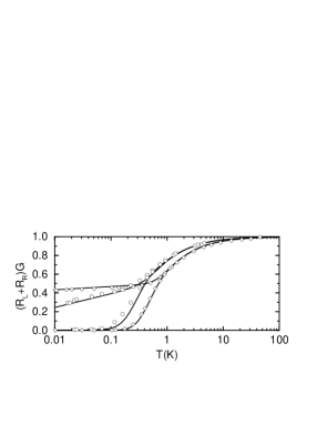
FIG. 5.: Maximal and minimal linear conductance for $E_{\rm C}=1.47K$ and $\alpha_{0}=0.015$, and $E_{\rm C}=1K$ and $\alpha_{0}=0.063$. The dots are experimental data from Ref. [14].

REFERENCES

- [1] D.V. Averin and K.K. Likharev, in Mesoscopic Phenomena in Solids, ed. B.L. Altshuler et al. (Elsevier, 1991), p. 173.
- [2] Single Charge Tunneling, NATO ASI Series 294, H. Grabert and M.H. Devoret, eds., (Plenum Press, 1992).
- [3] G. Schön, Single-Electron Tunneling, to be published in Quantum Processes and Dissipation, Chapter 4, eds. B. Kramer et al., (VCH Publishers).
- [4] D.V. Averin and Yu.V. Nazarov, Phys. Rev. Lett. 65, 2446 (1990); ibid. in Chapter 6 in Ref. [2].
- [5] L.J. Geerligs, D.V. Averin, and J.E. Mooij, Phys. Rev. Lett. 65, 3037 (1990); U. Meirav, M.A. Kastner, and S.J. Wind, Phys. Rev. Lett. 65, 771 (1990); Chapter 3,6 in Ref. [2].
- [6] H. Schoeller and G. Schön, Phys. Rev. B 50, 18436 (1994); Physica B 203, 423 (1994).
- [7] J. König, H. Schoeller and G. Schön, Europhys. Lett. 31, 31 (1995); and in Quantum Dynamics of Submicron Structures, eds. H. A. Cerdeira et al., NATO ASI Series E, Vol. 291 (Kluwer, 1995), p.221.
- [8] P. Lafarge et al., Z. Phys. B - Condensed Matter 85, 327 (1991).
- [9] K.A. Matveev, Sov. Phys. JETP 72, 892 (1991), [Zh. Eksp. Teor. Fiz. 99, 1598 (1991)].
- [10] D.S. Golubev and A.D. Zaikin, Phys. Rev. B 50, 8736 (1994).
- [11] G. Falci, G. Schön, and G.T. Zimanyi, Phys. Rev. Lett. 74, 3257 (1995).
- [12] J. König, H. Schoeller and G. Schön, Phys. Rev. Lett. 76, 1715 (1996); and in Festkörperprobleme / Advances in Solid State Physics, Vol. 35, ed. by R. Helbig (Vieweg, Braunschweig/Wiesbaden), p.215 (1996).
- [13] J. König, J. Schmid, H. Schoeller, and G. Schön, Phys. Rev. B 54, 16820 (1996).
- [14] P. Joyez, V. Bouchiat, D. Esteve, C. Urbina, and M.H. Devoret, submitted to Phys. Rev. Lett.
- [15] H. Grabert, Phys. Rev. B 50, 17364 (1994).
- [16] Usually, the value of the integral is approximated by replacing the denominators with an -independent term or by adding a constant finite life-time in the denominator, see e.g. Y.V. Nazarov, J. Low Temp. Phys. 90, 77 (1993) and D.V. Averin, Physica 194-196, 979 (1994).