Local perturbation in a Tomonaga-Luttinger liquid at $g=1/2$:
orthogonality catastrophe, Fermi-edge singularity, and local density of states

Abstract

The orthogonality catastrophe in a Tomonaga-Luttinger liquid with an impurity is reexamined for the case when the interaction parameter or the dimensionless conductance is $g=1/2$. By transforming bosons back to fermions, the Hamiltonian is reduced to a quadratic form, which allows for explicit calculation of the overlap integral and the local density of states at the defect site. The exponent of the orthogonality catastrophe due to a backward scattering center is found to be 1/8, in agreement with previous studies using different approaches. The time-dependence of the core-hole Green’s function is computed numerically, which shows a clear crossover from a non-universal short-time behavior to a universal long-time behavior. The local density of states vanishes linearly in the low-energy limit at $g=1/2$.

I Introduction

One-dimensional interacting fermion systems, Tomonaga-Luttinger (TL) liquids,[1, 2, 3] have recently attracted much attention due to their anomalous response to local perturbations. Recent extensive studies [4, 5, 6, 7, 8, 9] on transport properties of TL liquids with an impurity revealed that repulsively interacting fermions have vanishing transmission probability through a potential barrier in the low-energy limit. This is because the interaction between fermions strongly enhances the backward scattering at the barrier. Thus, a single defect effectively cuts a TL liquid into two disconnected ones at zero temperature.[4] This implies that the local density of states (LDOS) at the defect is reduced for low energy, and according to Kane and Fisher[4] it shows a power-law energy dependence,

$$\rho(\omega)\propto\omega^{\frac{1}{g}-1},$$ (1)

where $g$ is a parameter characterizing the TL liquid. This picture was, however, questioned recently by Oreg and Finkel’stein,[10] who claimed based on a mapping to a Coulomb gas problem that the LDOS at the defect is enhanced, rather than suppressed, in the low-energy limit for weakly interacting fermions. This controversy motivates us to reexamine this issue.

The orthogonality catastrophe[11] in a TL liquid is another interesting subject which has been discussed by several authors.[12, 13, 14, 15, 16, 17, 18] They showed that the overlap between the ground state of a pure TL liquid $|{\rm p}\rangle$ and that of a TL liquid with a single scatterer $|{\rm s}\rangle$ vanishes in the limit of large system size:

$$|\langle{\rm p}|{\rm s}\rangle|^{2}\propto L^{-\gamma_{F}-\gamma_{B}},$$ (2)

where $L$ is the length of the system. The exponent $\gamma_{F}$ is due to the forward-scattering potential and depends on its strength.[12, 13] It can be calculated directly using a unitary transformation. The other exponent $\gamma_{B}$ due to the backward scattering is believed to be independent of the strength of the potential and take a universal value, $1/8$.[14, 15, 16, 17] In Refs. [14, 15], and [17] the exponent $\gamma_{B}$ is calculated by assuming that a backward scattering center can be replaced with an impenetrable potential barrier. Oreg and Finkel’stein,[18] however, questioned the validity of the assumption and argued that the exponent of the Fermi-edge singularity due to a backward scattering center is zero, which implies $\gamma_{B}=0$. On the other hand, Kane et al.[16] used a renormalization-group equation which becomes exact in the limit of weak repulsive interaction between fermions. They could describe a crossover from the high-energy regime to the low-energy regime, and obtained the same exponent $\gamma_{B}=1/8$ in the low-energy limit. The result of a recent direct numerical calculation of the overlap integral[19] is also consistent with $\gamma_{B}=1/8$.

It is known that, when the TL-liquid parameter $g$ is 1/2, the bosonized Hamiltonian containing a nonlinear term representing the backward scattering can be transformed to a quadratic Hamiltonian of fermions.[20] This is essentially the same technique as the Emery-Kivelson solution of the two-channel Kondo problem.[22] The exact results on the conductance[4] and non-equilibrium noise spectra[21] were obtained using this refermionization technique. It is thus natural to expect that exact calculation should also be possible for the above-mentioned problems. The purpose of this paper is to show that this is indeed the case.

The structure of this paper is as follows. After introducing a model of interacting fermions in Sec. II, we discuss in Sec. III the exact low-energy behavior of the LDOS for $g=1/2$. For $g\neq 1/2$ we show that Eq. (1) follows from the assumption that the phase field is pinned at the defect site. The importance of zero-modes is emphasized. In Sec. IV we calculate $\gamma_{B}$ analytically for $g=1/2$ without assuming the nature of the low-energy fixed point. We find $\gamma_{B}=1/8$. The so-called core-hole Green’s function is then computed numerically in Sec. V, which shows a clear crossover from short-time to long-time regimes. We show in Sec. VI that the exponent of the Fermi-edge singularity due to backward scattering is also given by $\gamma_{B}$. We summarize the results in Sec. VII.

II Model

In this section we introduce a model of interacting spinless fermions and briefly explain the bosonization rule to fix the notation.

The Hamiltonian of our model is given by

                                                                           

$$H = iv_{F}\int^{\infty}_{-\infty}dx\left[\psi^{\dagger}_{L}(x)\frac{d}{dx}\psi_{L}(x)-\psi^{\dagger}_{R}(x)\frac{d}{dx}\psi_{R}(x)\right]+g_{2}\int^{\infty}_{-\infty}dx:\!\psi^{\dagger}_{L}(x)\psi_{L}(x)\!:\,:\!\psi^{\dagger}_{R}(x)\psi_{R}(x)\!:$$ (4)

$$+\frac{g_{4}}{2}\int^{\infty}_{-\infty}dx\sum_{\mu=L,R}:\!\psi^{\dagger}_{\mu}(x)\psi_{\mu}(x)\!::\!\psi^{\dagger}_{\mu}(x)\psi_{\mu}(x)\!:+\lambda_{F}\sum_{\mu=L,R}:\!\psi^{\dagger}_{\mu}(0)\psi_{\mu}(0)\!:+\lambda_{B}\!\left[e^{i\theta}\psi^{\dagger}_{L}(0)\psi_{R}(0)+{\rm h.c.}\right],$$

                                                                           

where $\psi_{L(R)}$ describes left-going (right-going) fermions, $:\!\!A\!\!:$ represents normal-ordered operator $A$, and $\lambda_{F}$ ($\lambda_{B}e^{i\theta}$) is the forward-scattering (backward-scattering) potential. Following the standard bosonization rule,[23] we express fermions $\psi_{\mu}$ in terms of bosonic operators:

$$\psi_{L}(x) = \frac{1}{\sqrt{2\pi\alpha}}\eta_{L}e^{-i\varphi_{L}(x)},$$ (6)

$$\psi_{R}(x) = \frac{1}{\sqrt{2\pi\alpha}}\eta_{R}e^{i\varphi_{R}(x)},$$ (7)

$$:\!\psi^{\dagger}_{\mu}(x)\psi_{\mu}(x)\!:\! = \frac{1}{2\pi}\frac{d}{dx}\varphi_{\mu}(x),$$ (8)

where $\alpha$ is a short-distance cutoff. The bosonic fields satisfy the commutation relations $[\varphi_{L}(x),\varphi_{L}(y)]=-i\pi{\rm sgn}(x-y)$, $[\varphi_{R}(x),\varphi_{R}(y)]=i\pi{\rm sgn}(x-y)$, and $[\varphi_{L}(x),\varphi_{R}(y)]=0$. The operator $\eta_{\mu}$’s are Majorana fermions corresponding to zero modes of bosons, which are needed to ensure the anticommutation relation between $\psi_{L}$ and $\psi_{R}$. They satisfy $\{\eta_{L},\eta_{R}\}=0$ and $\eta^{2}_{\mu}=1$. We then introduce new bosonic fields as

$$\phi(x) = \frac{1}{\sqrt{4\pi}}[\varphi_{R}(x)+\varphi_{L}(x)],$$ (10)

$$\Pi(x) = -\frac{1}{\sqrt{4\pi}}\frac{d}{dx}[\varphi_{R}(x)-\varphi_{L}(x)],$$ (11)

which obey $[\phi(x),\Pi(y)]=i\delta(x-y)$. With these fields the Hamiltonian can be transformed to a bosonic form,

$$H = \frac{v}{2}\int dx\left[\frac{1}{g}\left(\frac{d\phi}{dx}\right)^{2}+g\Pi^{2}\right]$$ (13)

$$+\frac{\lambda_{F}}{\sqrt{\pi}}\frac{d\phi(0)}{dx}+i\frac{\lambda_{B}}{\pi\alpha}\eta_{L}\eta_{R}\sin\left[\sqrt{4\pi}\phi(0)+\theta\right].$$

The parameter $g$ is related to $g_{2}$ and $g_{4}$ by $g=[(1+\tilde{g}_{4}-\tilde{g}_{2})/(1+\tilde{g}_{4}+\tilde{g}_{2})]^{1/2}$ with $\tilde{g}_{i}=g_{i}/2\pi v_{F}$. Since the interaction is repulsive, $g$ is less than 1. The renormalized velocity is given by $v=v_{F}[(1+\tilde{g}_{4})^{2}-(\tilde{g}_{2})^{2}]^{1/2}$.

                                                                           

We then introduce another set of bosonic fields $\varphi_{\pm}(x)$:[17]

$$\varphi_{\pm}(x)=\frac{1}{\sqrt{8}}\left\{\left(\frac{1}{\sqrt{g}}-\sqrt{g}\right)[\varphi_{R}(x)\pm\varphi_{L}(-x)]+\left(\frac{1}{\sqrt{g}}+\sqrt{g}\right)[\varphi_{R}(-x)\pm\varphi_{L}(x)]\right\}.$$ (14)

These fields satisfy $[\varphi_{+}(x),\varphi_{+}(y)]=[\varphi_{-}(x),\varphi_{-}(y)]=-i\pi{\rm sgn}(x-y)$ and $[\varphi_{+}(x),\varphi_{-}(y)]=0$. The advantage of using $\varphi_{\pm}$ is that we may separate the Hamiltonian into two commuting parts, $H=H_{F}+H_{B}$, where

$$H_{F} = \frac{v}{4\pi}\int^{\infty}_{-\infty}dx\left(\frac{d\varphi_{-}}{dx}\right)^{2}+\frac{\lambda_{F}}{\pi}\sqrt{\frac{g}{2}}\frac{d\varphi_{-}(0)}{dx},$$ (15)

$$H_{B} = \frac{v}{4\pi}\int^{\infty}_{-\infty}dx\left(\frac{d\varphi_{+}}{dx}\right)^{2}+i\frac{\lambda_{B}}{\pi\alpha}\eta_{L}\eta_{R}\sin\left[\sqrt{2g}\varphi_{+}(0)+\theta\right].$$ (16)

The fermion field at $x=0$ may be written as

$$\psi(0)=\frac{1}{\sqrt{2\pi\alpha}}\exp\left[-\frac{i}{\sqrt{2g}}\varphi_{-}(0)\right]\left\{\eta_{L}\exp\left[-i\sqrt{\frac{g}{2}}\varphi_{+}(0)\right]+\eta_{R}\exp\left[i\sqrt{\frac{g}{2}}\varphi_{+}(0)\right]\right\}.$$ (17)

III Local density of states at a scattering center

In this section we calculate the following correlation function:

$$D(t)\equiv\langle g_{\theta}|e^{iHt}\psi^{\dagger}(0)e^{-iHt}\psi(0)|g_{\theta}\rangle,$$ (18)

where $|g_{\theta}\rangle$ is a ground state of $H$. The LDOS is given by $\rho(\omega)=\int(d\omega/2\pi)e^{i\omega t}D(t)$. In general we expect $D(t)\propto e^{-i\Delta t}t^{-\nu}$ for $t\to\infty$. Since $H$ has gapless excitations, we know that $\Delta$ must be zero. Thus, we will not pay attention to $\Delta$ and concentrate only on the exponent $\nu$ in the following discussion.

Since $H_{F}$ and $H_{B}$ commute, the correlation function is factorized into two parts as $D(t)=\frac{1}{2\pi\alpha}D_{F}(t)D_{B}(t)$, where

$$D_{F}(t) = \langle{\rm F}|e^{iH_{F}t}e^{i\Phi_{-}}e^{-iH_{F}t}e^{-i\Phi_{-}}|{\rm F}\rangle,$$ (20)

$$D_{B}(t) = \langle{\rm B}|e^{iH_{B}t}\left(\eta_{L}e^{i\Phi_{+}}+\eta_{R}e^{-i\Phi_{+}}\right)e^{-iH_{B}t}\left(\eta_{L}e^{-i\Phi_{+}}+\eta_{R}e^{i\Phi_{+}}\right)|{\rm B}\rangle,$$ (21)

Here $\Phi_{-}=\varphi_{-}(0)/\sqrt{2g}$, $\Phi_{+}=\sqrt{g/2}\varphi_{+}(0)$, and $|{\rm F}\rangle$ ($|{\rm B}\rangle$) is a ground states of $H_{F}$ ($H_{B}$). The Hamiltonian $H_{F}$ is related to a free Hamiltonian by a unitary transformation as $UH_{F}U^{\dagger}=H_{F}^{(0)}+{\rm const}$, where

$$H_{F}^{(0)}=\frac{v}{4\pi}\int^{\infty}_{-\infty}dx\left(\frac{d\varphi_{-}}{dx}\right)^{2}$$ (22)

and

$$U=\exp\left[-i\frac{\lambda_{F}}{\pi v}\sqrt{\frac{g}{2}}\varphi_{-}(0)\right].$$ (23)

This means $|F\rangle=U^{\dagger}|F_{0}\rangle$ with $|F_{0}\rangle$ being the ground state of $H_{F}^{(0)}$. We thus get

$$D_{F}(t)=\langle F_{0}|e^{iH_{F}^{(0)}t}e^{i\Phi_{-}}e^{-iH_{F}^{(0)}t}e^{-i\Phi_{-}}|F_{0}\rangle=\left(1+i\frac{vt}{\alpha}\right)^{-\frac{1}{2g}}\sim t^{-\frac{1}{2g}}.$$ (24)

As pointed out in Ref. [10], the forward-scattering potential does not affect the LDOS.

Next we rewrite Eq. (21) as

$$D_{B}(t)=\langle B|e^{iH_{B}t}\left(e^{i\Phi_{+}}-\eta_{L}\eta_{R}e^{-i\Phi_{+}}\right)e^{-i\widetilde{H}_{B}t}\left(e^{-i\Phi_{+}}+\eta_{L}\eta_{R}e^{i\Phi_{+}}\right)|B\rangle,$$ (25)

                                                                           

where $\widetilde{H}_{B}\equiv\eta_{L}H_{B}\eta_{L}=H_{B}(\lambda_{B}\to-\lambda_{B})$. Note that this sign change of the cosine term is a direct consequence of the anticommutation relation $\{\psi_{L},\psi_{R}\}=0$. At this point we may set $\eta_{L}\eta_{R}=-i$ because only the terms involving even powers of $\eta_{L}\eta_{R}$ will contribute to $D_{B}(t)$ when Eq. (25) is calculated perturbatively in powers of $\lambda_{B}$. We then shift $\varphi_{+}(x)\to\varphi_{+}(x)+\frac{1}{\sqrt{2g}}(\frac{\pi}{2}-\theta)$ and obtain

$$D_{B}(t) = 2\langle+|e^{iH_{+}t}e^{i\Phi_{+}}e^{-iH_{-}t}e^{-i\Phi_{+}}|+\rangle$$ (28)

$$+2\cos\theta\langle+|e^{iH_{+}t}e^{i\Phi_{+}}e^{-iH_{-}t}e^{i\Phi_{+}}|+\rangle,$$

where

$$H_{\pm}\equiv\frac{v}{4\pi}\int^{\infty}_{-\infty}dx\left(\frac{d\varphi_{+}}{dx}\right)^{2}\pm\frac{\lambda_{B}}{\pi\alpha}\cos\left[\sqrt{2g}\varphi_{+}(0)\right]$$ (29)

and we have used the fact that the ground state of $H_{+}$, $|+\rangle$, is invariant under $\varphi_{+}\to-\varphi_{+}$. It is useful to transform Eq. (28) further to the form

$$D_{B}(t) = 2\langle+|e^{iH_{+}t}e^{-i\widetilde{H}_{-}t}|+\rangle$$ (31)

$$+2\cos\theta\langle+|e^{iH_{+}t}e^{-i\widetilde{H}_{-}t}e^{2i\Phi_{+}}|+\rangle,$$

where

$$\widetilde{H}_{-} = \frac{v}{4\pi}\int^{\infty}_{-\infty}dx\left(\frac{d\varphi_{+}}{dx}-\pi\sqrt{2g}\delta(x)\right)^{2}$$ (33)

$$-\frac{\lambda}{\pi\alpha}\cos\left[\sqrt{2g}\varphi_{+}(0)\right].$$

We first consider the case of $g=1/2$. A crucial point in this case is that the cosine term becomes $e^{i\varphi_{+}(0)}+e^{-i\varphi_{+}(0)}$. Therefore, fermionizing the chiral boson $\varphi_{+}$ as

$$\frac{e^{i\varphi_{+}(x)}}{\sqrt{2\pi\alpha}}=\eta\psi_{+}(x),$$ (34)

we may transform Eq. (29) to[20, 24]

$$H_{\pm} = iv\int^{\infty}_{-\infty}dx\psi^{\dagger}_{+}(x)\frac{d}{dx}\psi_{+}(x)$$ (36)

$$\pm\frac{\lambda_{B}}{\sqrt{2\pi\alpha}}\left[\eta\psi_{+}(0)+\psi^{\dagger}_{+}(0)\eta\right],$$

where $\eta$ is a Majorana fermion, satisfying $\eta^{2}=1$. This leads to a simple relation, $\eta H_{+}\eta=H_{-}$. Note that $H_{+}$ is a quadratic Hamiltonian, which can be easily diagonalized:[20]

$$H_{+} = \int^{\infty}_{-\infty}dk\left[\xi_{k}a_{k}^{\dagger}a_{k}+\frac{\lambda_{B}}{2\pi\sqrt{\alpha}}\left(\eta a_{k}+a_{k}^{\dagger}\eta\right)\right]$$ (37)

$$= \int^{\infty}_{0}dk\xi_{k}\left(c^{\dagger}_{k}c_{k}+d^{\dagger}_{k}d_{k}\right)+{\rm const},$$ (38)

where $\xi_{k}\equiv vk$ and $\psi_{+}(x)=\int(dk/\sqrt{2\pi})e^{-ikx}a_{k}$. For later convenience we write the transformation rule here:[20]

                                                                           

$$a_{k} = \frac{1}{\sqrt{2}}c_{k}+\frac{\xi_{k}}{\sqrt{2(\xi^{2}_{k}+\Gamma^{2})}}d_{k}+\frac{\Gamma}{\sqrt{2}\pi}{\rm P}\!\!\int^{\infty}_{0}dq\frac{1}{\sqrt{\xi^{2}_{q}+\Gamma^{2}}}\left(\frac{d_{q}}{q-k}-\frac{d^{\dagger}_{q}}{q+k}\right),$$ (40)

$$a_{-k} = \frac{1}{\sqrt{2}}c^{\dagger}_{k}-\frac{\xi_{k}}{\sqrt{2(\xi^{2}_{k}+\Gamma^{2})}}d^{\dagger}_{k}+\frac{\Gamma}{\sqrt{2}\pi}{\rm P}\!\!\int^{\infty}_{0}dq\frac{1}{\sqrt{\xi^{2}_{q}+\Gamma^{2}}}\left(\frac{d_{q}}{q+k}-\frac{d^{\dagger}_{q}}{q-k}\right),$$ (41)

$$\eta = \frac{\lambda_{B}}{\pi}\sqrt{\frac{2}{\alpha}}\,{\rm P}\!\!\int^{\infty}_{0}dq\frac{1}{\sqrt{\xi^{2}_{q}+\Gamma^{2}}}\left(d_{q}+d^{\dagger}_{q}\right),$$ (42)

where $k>0$, $\Gamma\equiv\lambda^{2}_{B}/(\pi\alpha v)$, and $c_{k}$ and $d_{k}$ satisfy the ordinary anticommutation relation. The ground state $|+\rangle$ is the vacuum of $c_{k}$ and $d_{k}$.

Using Eq. (34), we rewrite Eq. (31) in a fermionic form,

$$D_{B}(t)=2\langle+|e^{iH_{+}t}\eta e^{-i\widetilde{H}_{+}t}\eta|+\rangle+2\sqrt{2\pi\alpha}\cos\theta\langle+|e^{iH_{+}t}\eta e^{-i\widetilde{H}_{+}t}\psi_{+}(0)|+\rangle,$$ (43)

where

$$\widetilde{H}_{+}=H_{+}+\pi v:\!\psi_{+}^{\dagger}(0)\psi_{+}(0)\!:+{\rm const}.$$ (44)

From Eqs. (40) and (41), the second term becomes

$$\pi v:\!\psi^{\dagger}_{+}(0)\psi_{+}(0)\!:\,\,=\frac{v}{2}\int^{\infty}_{0}dk\int^{\infty}_{0}dp\frac{\xi_{p}}{\sqrt{\xi^{2}_{p}+\Gamma^{2}}}\left(c_{k}+c^{\dagger}_{k}\right)\left(d_{p}-d^{\dagger}_{p}\right),$$ (45)

                                                                           

which is an irrelevant operator with scaling dimension 2. To find the long-time behavior of $D_{B}(t)$, we can thus treat Eq. (45) as a small perturbation. The lowest-order calculation then gives, for $\Gamma t\gg 1$,

$$D_{B}(t)=-\frac{4i}{\pi\Gamma t}+\sqrt{2\pi\alpha}\cos\theta\frac{\lambda_{B}}{\pi v}\frac{\ln(vt/\alpha)}{\Gamma^{2}t^{2}}.$$ (46)

Note that the $1/t$-dependence of the first term comes from the correlator $\langle+|\eta(t)\eta(0)|+\rangle$, which also appeared in the two-channel Kondo problem.[22] Combining Eqs. (24) and (46), we get $D(t)=-2/(\pi^{2}v\Gamma t^{2})$ for $\Gamma t\gg 1$, which implies

$$\rho(\omega)=\frac{2\omega}{\pi^{2}v\Gamma}$$ (47)

for $\omega\ll\Gamma$. This is consistent with Eq. (1). We see that the single scatterer at $x=0$ indeed depletes the low-energy excitations around it.

For $g\neq 1/2$ ($0<g<1$) we take a different approach. We assume from the outset that the phase field $\varphi_{+}$ is pinned at $x=0$ by the cosine potential in $H_{+}$ (29), as in Refs. [14, 15], and [17]. We thus replace the cosine by a term which is easier to deal with. A convenient choice is

$$H_{M}=\frac{v}{2}\int^{\infty}_{-\infty}dx\left[\frac{1}{g}\left(\frac{d\phi}{dx}\right)^{2}+g\Pi^{2}\right]+\frac{M}{2}[\phi(0)]^{2},$$ (48)

where $M$ should be a characteristic energy scale at which the cosine term becomes of the order of the band width ($M=\Gamma$ for $g=1/2$). It immediately follows from the scaling equation $d\lambda_{B}/dl=(1-g)\lambda_{B}$ that

$$M\propto\frac{v}{\alpha}\left(\frac{\lambda_{B}}{v}\right)^{\frac{1}{1-g}}.$$ (49)

Since $H_{M}$ is a quadratic Hamiltonian, it is easily diagonalized as $H_{M}=\int dk\xi_{k}\left(\alpha^{\dagger}_{k}\alpha_{k}+\beta^{\dagger}_{k}\beta_{k}\right)$ with

$$\phi=\int^{\infty}_{0}dk\sqrt{\frac{g}{2\pi k}}\left[\sin(kx)\left(\alpha_{k}+\alpha_{k}^{\dagger}\right)+\cos(k|x|-\delta_{k})\left(\beta_{k}+\beta_{k}^{\dagger}\right)\right]$$ (50)

and $\Pi=(1/gv)\partial\Pi/\partial t$, where $\alpha_{k}$ and $\beta_{k}$ satisfy the ordinary commutation relations of bosons. The phase shift is given by $\delta_{k}=\tan^{-1}(gM/2vk)$. Note that $\delta_{k}\to\pi/2$ as $k\to 0$.

Let us denote the ground state of $H_{M}$ by $|0_{M}\rangle$. We then find

$$\langle 0_{M}|\partial_{x}\varphi_{+}(0,t)\,\partial_{x}\varphi_{+}(0,0)|0_{M}\rangle=2\pi g\langle 0_{M}|\Pi(0,t)\Pi(0,0)|0_{M}\rangle=\frac{24}{g^{2}M^{2}v^{2}t^{4}}$$ (51)

                                                                           

for $Mt\gg 1$, implying that $\partial_{x}\varphi_{+}(0)$ is an irrelevant operator with dimension 2. This is consistent with the observation made in Eq. (45). In fact, this is an expected result because $\varphi_{+}$ is pinned at $x=0$. We may thus use $H_{-}$ instead of $\widetilde{H}_{-}$ to obtain the long-time asymptotic behavior of $D_{B}(t)$ in Eq. (31). It is also important to note that $e^{i\Phi_{+}}$ is not fluctuating too much and can be regarded essentially as a constant because $\varphi_{+}(0)$ is pinned. In fact, we find

$$\langle 0_{M}|e^{i\Phi_{+}}|0_{M}\rangle = \langle 0_{M}|\exp\left[i\sqrt{2\pi/g}\phi(0)\right]|0_{M}\rangle$$ (52)

$$= \sqrt{\frac{e^{\gamma}g\alpha M}{2v}}$$ (53)

for $\alpha M\ll v$, where $\gamma=0.577\ldots$ is Euler’s constant. Note that, at $g=1/2$, we get $\langle+|e^{i\Phi_{+}}|+\rangle=-(\lambda_{B}/\pi v)\ln(v/\alpha\Gamma)$, which is consistent with Eqs. (49) and (53). Hence, from Eq. (31), we get

$$D_{B}(t) \propto \langle 0_{M}|e^{iH_{+}t}Ve^{-iH_{+}t}V^{\dagger}|0_{M}\rangle$$ (54)

$$\approx \langle 0_{M}|e^{iH_{M}t}Ve^{-iH_{M}t}V^{\dagger}|0_{M}\rangle,$$ (55)

where $V$ is a unitary operator which shifts $\phi(x)\to\phi(x)+\frac{\sqrt{\pi}}{2}$. The rhs of Eq. (55) is known to decay as $\sim t^{-1/2g}$.[25] This result can be easily obtained using the following representation for $V$:

$$V = \exp\left[i\frac{\sqrt{\pi}}{2}\int dx\Pi(x)\right]$$ (56)

$$= \exp\left[-\int^{\infty}_{0}dk\frac{e^{-\alpha k}}{\sqrt{2gk}}\sin\delta_{k}\left(\beta^{\dagger}_{k}-\beta_{k}\right)\right].$$ (57)

We therefore conclude $D(t)\propto t^{-1/g}$, from which Eq. (1) follows. We emphasize that the above calculation should give the exact value of the exponent, although the amplitude may not be correct.

IV Orthogonality catastrophe

In this section we discuss the orthogonality catastrophe for the special case of $g=1/2$. We calculate the overlap integral $|\langle{\rm p}|{\rm s}\rangle|^{2}=|\langle F_{0}|F\rangle|^{2}\times|\langle 0|+\rangle|^{2}$, where $|0\rangle$ is the ground state of the Hamiltonian $H_{0}\equiv H_{+}|_{\lambda_{B}=0}$. It is almost trivial to find $\gamma_{F}$ in Eq. (2) because $\langle F_{0}|F\rangle=\langle F_{0}|U^{\dagger}|F_{0}\rangle$. We get[12, 13]

$$\gamma_{F}=2g\left(\frac{\lambda_{F}}{2\pi v}\right)^{2}.$$ (58)

Hence our problem is reduced to calculate the overlap $\langle 0|+\rangle$. In the fermion language, $H_{0}$ is

$$H_{0}=iv\int^{\infty}_{-\infty}dx\psi^{\dagger}_{+}(x)\frac{d}{dx}\psi_{+}(x),$$ (59)

and $|0\rangle$ is the filled Fermi sea. Then the ground state of $H_{+}$ can be written as

$$|+\rangle={\rm T}\exp\left[-i\int^{0}_{-\infty}e^{\epsilon t}H^{\prime}(t)dt\right]|0\rangle,$$ (60)

where $\epsilon$ is positive infinitesimal and $H^{\prime}(t)=e^{iH_{0}t}(H_{+}-H_{0})e^{-iH_{0}t}$. Using the linked-cluster theorem, we can write the overlap integral as

$$\langle 0|+\rangle=\exp[G_{c}(0,-\infty)],$$ (61)

where $G_{c}(0,-\infty)$ is a sum of connected ring diagrams,

                                                                           

$$G_{c}(0,-\infty) = -\sum^{\infty}_{n=1}\frac{\lambda^{2n}}{2n}\int^{0}_{-\infty}\!\!dt_{1}\cdots\int^{0}_{-\infty}\!\!dt_{2n}s_{0}(t_{1}-t_{2})g_{0}(t_{2}-t_{3})\cdots s_{0}(t_{2n-1}-t_{2n})g_{0}(t_{2n}-t_{1})\exp\!\left(\sum^{2n}_{i=1}\epsilon t_{i}\right).$$ (62)

Here $\lambda\equiv\lambda_{B}/\sqrt{2\pi\alpha}$ and the propagators $s_{0}(t)$ and $g_{0}(t)$ are given by

$$s_{0}(t) = \langle 0|{\rm T}\eta(t)\eta(0)|0\rangle={\rm sgn}(t),$$ (64)

$$g_{0}(t) = \langle 0|{\rm T}[\psi_{+}(x=0,t)-\psi^{\dagger}_{+}(0,t)][\psi_{+}(0,0)-\psi^{\dagger}_{+}(0,0)]|0\rangle=\frac{i}{\pi v[t-i\varepsilon{\rm sgn}(t)]},$$ (65)

where $\varepsilon$ is positive infinitesimal. Differentiating Eq. (62) with respect to $\lambda$, we obtain

$$G_{c}(0,-\infty)=-\frac{v}{4}\int^{\Gamma}_{0}d\Gamma\int^{0}_{-\infty}dt_{1}\int^{0}_{-\infty}dt_{2}e^{\epsilon(t_{1}+t_{2})}s_{0}(t_{1}-t_{2})g(t_{2},t_{1}),$$ (66)

where $g(t_{1},t_{2})$ is a solution of a Dyson equation,

$$g(t_{1},t_{2})=g_{0}(t_{1}-t_{2})-\frac{\Gamma}{2\pi i}{\rm P}\!\!\int^{0}_{-\infty}\!\!dt_{3}\int^{0}_{-\infty}\!\!dt_{4}\frac{e^{\epsilon(t_{3}+t_{4})}}{t_{1}-t_{3}}{\rm sgn}(t_{3}-t_{4})g(t_{4},t_{2}).$$ (67)

Since Eq. (67) contains double integral, working in real time is not so convenient as it is in the Fermi-liquid case.[26] On the other hand, the Fourier transform of Eq. (67) contains only a single integral:

$$\tilde{g}(\omega,t_{2})=-\frac{e^{i\omega t_{2}}}{v}{\rm sgn}(\omega)+\frac{i\Gamma}{|\omega|}\int^{\infty}_{-\infty}\frac{d\nu}{2\pi i}\tilde{g}(\nu,t_{2})\left[\frac{1}{\nu-\omega+2i\epsilon}-\frac{1}{2(\nu+i\epsilon)}\right].$$ (68)

This equation can be solved in the limit $\epsilon\to 0$ in the standard way.[27]

We first introduce functions $\tilde{g}_{\pm}$ by

$$\tilde{g}_{\pm}(\omega)=\int^{\infty}_{-\infty}\frac{d\nu}{2\pi i}\tilde{g}(\nu,t_{2})\left[\frac{1}{\nu-\omega\mp 2i\epsilon}-\frac{1}{2(\nu+i\epsilon)}\right].$$ (69)

We can then express Eq. (68) as

$$\tilde{g}_{+}(\omega)-\left(1-i\frac{\Gamma}{|\omega|}\right)\tilde{g}_{-}(\omega)=-\frac{e^{i\omega t_{2}}}{v}{\rm sgn}(\omega).$$ (70)

A solution of this equation with correct analytic properties is

$$\tilde{g}_{\pm}(\omega)=-\frac{1}{v}\int^{\infty}_{-\infty}\!\frac{d\nu}{2\pi i}\frac{e^{i\nu t_{2}}{\rm sgn}(\nu)}{\nu-\omega\mp i\delta}\frac{X_{\pm}(\omega)}{X_{+}(\nu)},$$ (71)

where $\delta$ is positive infinitesimal and

$$X_{\pm}(\omega)=\exp\!\left[\int^{\infty}_{-\infty}\!\frac{d\nu}{2\pi i}\frac{\ln\left(1-i\frac{\Gamma}{|\nu|}\right)}{\nu-\omega\mp i\delta}\right].$$ (72)

With this solution Eq. (66) becomes

$$G_{c}(0,-\infty) = \frac{1}{8\pi^{2}i}\int^{\Gamma}_{0}\!\!d\Gamma\int^{0}_{-\infty}\!\!dt_{1}\!\int^{t_{1}}_{-\infty}\!\!dt_{2}\!\int^{\infty}_{-\infty}\!\!d\omega\!\int^{\infty}_{-\infty}\!\!d\nu\,e^{-i\omega t_{1}+i\nu t_{2}+\epsilon(t_{1}+t_{2})}\frac{{\rm sgn}(\nu)}{\nu-\omega+i\delta}\frac{X_{-}(\omega)}{X_{+}(\nu)}$$ (73)

$$= \frac{1}{8\pi^{2}}\int^{\Gamma}_{0}\!\!d\Gamma\int^{0}_{-\infty}\!\!d\tau\!\int^{\infty}_{-\infty}\!\!d\nu\,e^{i(\nu-i\epsilon)\tau}\frac{{\rm sgn}(\nu)}{X_{+}(\nu)}\int^{\infty}_{-\infty}\!\!d\omega\frac{X_{-}(\omega)}{(\omega-\nu+2i\epsilon)(\nu-\omega+i\delta)},$$ (74)

where $\tau=t_{2}-t_{1}$ and we have integrated over $(t_{1}+t_{2})/2$. As pointed out by Hamann,[28] in the next step in which we perform the $\omega$ integral, it is important to keep $\epsilon$ finite while taking the limit $\delta\to+0$:

$$G_{c}(0,-\infty) = -\frac{i}{4\pi}\int^{\Gamma}_{0}\!\!d\Gamma\!\int^{0}_{-\infty}\!\!d\tau\!\int^{\infty}_{-\infty}\!\!d\nu e^{i(\nu-i\epsilon)\tau}\frac{{\rm sgn}(\nu)}{2i\epsilon}\frac{X_{-}(\nu-2i\epsilon)}{X_{+}(\nu)}$$

$$= -\frac{1}{8\pi\epsilon}\int^{\Gamma}_{0}\!\!d\Gamma\!\int^{0}_{-\infty}\!\!d\tau\!\int^{\infty}_{-\infty}\!\!d\nu\frac{\nu e^{i(\nu-i\epsilon)\tau}}{|\nu|-i\Gamma}+\frac{1}{8\pi^{2}}\int^{\Gamma}_{0}\!\!d\Gamma\!\int^{0}_{-\infty}\!\!d\tau\!\int^{\infty}_{-\infty}\!\!d\nu_{1}\!\int^{\infty}_{-\infty}\!\!d\nu_{2}\frac{\nu_{1}e^{i(\nu_{1}-i\epsilon)\tau}}{|\nu_{1}|-i\Gamma}\frac{\ln\left(1-i\frac{\Gamma}{|\nu_{2}|}\right)}{(\nu_{2}-\nu_{1}+i\delta)^{2}}.$$

After replacing $\nu/(|\nu|-i\Gamma)$ by $\nu[(|\nu|-i\Gamma)^{-1}-(\nu-i\Gamma)^{-1}]$ and $\ln\bigl{(}1-i\frac{\Gamma}{|\nu|}\bigr{)}$ by $\ln\bigl{[}\bigl{(}1-i\frac{\Gamma}{|\nu|}\bigr{)}/\left(1+i\frac{\Gamma}{\nu}\right)\bigr{]}$, we integrate over $\tau$ to obtain

$$G_{c}(0,-\infty) = \frac{1}{4\pi\epsilon i}\int^{\Gamma}_{0}\!\!d\Gamma\!\int^{0}_{-\infty}\!\!d\nu\frac{\nu}{\nu^{2}+\Gamma^{2}}-\frac{1}{2\pi^{2}}\int^{\Gamma}_{0}\!\!d\Gamma\!\int^{\infty}_{0}\!\!d\nu_{1}\!\int^{\infty}_{0}\!\!d\nu_{2}\frac{1}{(\nu_{1}+\nu_{2})^{2}}\frac{\nu_{1}}{\nu_{1}^{2}+\Gamma^{2}}\tan^{-1}\left(\frac{\Gamma}{\nu_{2}}\right)$$ (75)

$$= \frac{i}{2\epsilon}\frac{\Gamma}{2\pi}\left[\ln\!\left(\frac{\Lambda}{\Gamma}\right)+1\right]-\frac{1}{16}\ln\!\left(\frac{\Gamma}{E_{L}}\right),$$ (76)

where we have introduced the high-energy cutoff $\Lambda\sim v/\alpha$ and the low-energy cutoff $E_{L}\sim v/L$. From Eqs. (61) and (76) we get $\gamma_{B}=1/8$ in agreement with the previous studies.[14, 15, 16, 17, 19] Note that the quantity $E_{0}\equiv-(\Gamma/2\pi)[\ln(\Lambda/\Gamma)+1]$ appearing in the first term is equal to the difference between the ground state energies of $H_{+}$ and $H_{0}$.[20]

Since $\delta(E)\equiv\tan^{-1}(\Gamma/E)$ in Eq. (76) is the phase shift for fictitious chiral fermions due to the coupling $\lambda_{B}$ in Eq. (36), the above calculation implies that $\gamma_{B}=\frac{1}{2}[\delta(0)/\pi]^{2}$, in contrast to the Fermi-liquid result[11, 26] $\gamma_{\rm Fermi}=[\delta(0)/\pi]^{2}$. The extra factor $1/2$ in our result can be traced back to the peculiar form of the scattering term in Eq. (36). Only the combination $\psi_{+}-\psi^{\dagger}_{+}$ interacts with $\eta$, and the other combination $\psi_{+}+\psi^{\dagger}_{+}$ is decoupled. Hence only half of the degrees of freedom have the phase shift ($\delta(0)=\pi/2$), giving the factor $1/2$.

As pointed out by Matveev,[20] the Hamiltonian (36) is equivalent to the effective Hamiltonian of the two-channel Kondo model in the Toulouse limit,[22] where the Majorana fermion $\eta$ corresponds to the $xy$-component of the impurity spin. Thus our calculation also applies to the orthogonality catastrophe in the two-channel Kondo problem in which $J_{\perp}$ is turned on and off while $J_{z}$ kept constant.

V Core-hole Green’s function

Next we calculate the core-hole Green’s function,

$$G(t)=\langle 0|e^{iH_{0}t}e^{-iH_{+}t}|0\rangle$$ (77)

for $g=1/2$. Using the linked-cluster theorem again, we get $G(t)=\exp[G_{c}(t,0)]$, where $G_{c}(t,0)$ is

$$G_{c}(t,0)=-\sum^{\infty}_{n=1}\frac{\lambda^{2n}}{2n}\int^{t}_{0}\!\!dt_{1}\cdots\int^{t}_{0}\!\!dt_{2n}s_{0}(t_{1}-t_{2})g_{0}(t_{2}-t_{3})\cdots s_{0}(t_{2n-1}-t_{2n})g_{0}(t_{2n}-t_{1}).$$ (78)

                                                                           

This time we differentiate Eq. (78) with respect to $t$ to get

$$-\frac{d}{dt}G_{c}(t,0)=\lambda^{2}\int^{t}_{0}\!\!dt_{1}g_{0}(t-t_{1})s(t_{1}),$$ (79)

where $s(t_{1})$ is defined for $0\leq t_{1}\leq t$ and is a solution of a Dyson equation,

$$s(t_{1})=-1-\frac{\Gamma}{2\pi i}{\rm P}\!\!\int^{t}_{0}\!\!dt_{3}\!\int^{t}_{0}\!\!dt_{4}\frac{{\rm sgn}(t_{1}-t_{3})}{t_{3}-t_{4}}s(t_{4}).$$ (80)

From this equation we can easily show that $s(t_{1})=s(t-t_{1})$ and $s(+0)=-1$. Thus Eq. (79) becomes

$$-\frac{d}{dt}G_{c}(t,0)=\frac{\Gamma}{4}-\frac{\Gamma}{2\pi i}\int^{t}_{0}\!\!dt_{1}\frac{s(t_{1})}{t_{1}}.$$ (81)

Here the first term comes from the real part of $g_{0}$ in Eq. (65).

For short times $\Gamma t\ll 1$, we can solve Eq. (80) perturbatively. Up to order $(\Gamma t)^{2}$ we obtain

$$G_{c}(t,0)=i\frac{\Gamma t}{2\pi}\left[\ln\!\left(\frac{t}{t_{c}}\right)-1\right]-\frac{1}{4}\Gamma t+\frac{1}{24}(\Gamma t)^{2},$$ (82)

where $t_{c}$ is a short-time cutoff $\sim 1/\Lambda$. This expansion, however, starts to fail around $\Gamma t\sim 1$. From the analysis in Sec. IV, for $\Gamma t\gg 1$ we expect $G_{c}(t,0)$ to approach $-iE_{0}t-\frac{1}{8}\ln(\Gamma t)$.[14, 15, 16, 17]

The crossover from the short-time to the long-time regimes can be seen most conveniently by solving Eq. (80) numerically and putting the solution into Eq. (81). Note that the integral in Eq. (81) is well-defined because ${\rm Im}s(t_{1})\sim t_{1}|\ln t_{1}|$ for $t_{1}\to 0$. Figure 1 shows the $t$-dependence of the real part of $(d/dt)G_{c}(t,0)$ computed in this way. It clearly exhibits the crossover at $\Gamma t\sim 1$ from the short-time behavior, Eq. (81), to the long-time asymptote, ${\rm Re}[dG_{c}(t,0)/dt]=-1/8t$.

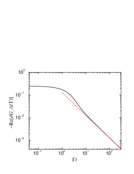
FIG. 1.: Time evolution of the core-hole Green’s function. There is a clear crossover at $\Gamma t\sim 1$. The dashed line represents ${\rm Re}[dG_{c}/d\Gamma t]=-1/(8\Gamma t)$.

VI Fermi-edge singularity

In this section we briefly discuss the Fermi-edge singularity for $g<1$ to show that the exponents can be easily obtained from the analysis of Secs. IV and V. Here we are concerned with the correlation function

$$I(t)=\langle g_{0}|e^{i(H_{F}^{(0)}+H_{0})t}\psi(0)e^{-i(H_{F}+H_{B})t}\psi^{\dagger}(0)|g_{0}\rangle,$$ (83)

where $|g_{0}\rangle\equiv|F_{0}\rangle\otimes|0\rangle$. Following the same path as in Sec. III, we write the correlator as $I(t)=\frac{1}{2\pi\alpha}I_{F}(t)I_{B}(t)$, where[12, 13]

$$I_{F}(t) = \langle F_{0}|e^{iH_{F}^{(0)}t}e^{-i\Phi_{-}}Ue^{-iH_{F}^{(0)}t}U^{\dagger}e^{i\Phi_{-}}|F_{0}\rangle$$ (84)

$$\sim t^{-\nu_{F}}$$ (85)

with $\nu_{F}=\left(\frac{1}{\sqrt{2g}}+\frac{\lambda_{F}}{2\pi v}\sqrt{2g}\right)^{2}$ and

$$I_{B}(t) = 2\langle 0|e^{iH_{0}t}e^{-i\widetilde{H}_{-}t}|0\rangle$$ (87)

$$+2\cos\theta\langle 0|e^{iH_{0}t}e^{-i\widetilde{H}_{-}t}e^{2i\Phi_{+}}|0\rangle.$$

We expect that $I_{B}(t)$ should decay as $I_{B}(t)\propto t^{-\nu_{B}}$ in the long-time limit. We now notice that the first term in Eq. (87) is similar to the core-hole Green’s function discussed in Sec. V. As we saw in Fig. 1, it should decay as $\sim t^{-\tilde{\gamma}}$ with $\tilde{\gamma}$ being the exponent of the orthogonality catastrophe between $|0\rangle$ and the ground state of $\widetilde{H}_{-}$: $|\langle 0|-\rangle|^{2}\propto L^{-\tilde{\gamma}}$. The latter state has a finite overlap with the ground state of $H_{-}$, because $\partial_{x}\varphi(0)$ $[\propto(\widetilde{H}_{-}-H_{-})]$ is an irrelevant operator around the fixed point of $H_{-}$. This means $\tilde{\gamma}=\gamma_{B}=1/8$. Since the second term in Eq. (87) contains extra factor, $e^{2i\Phi_{+}}$, at least it is not larger than the first term. Hence we conclude $\nu_{B}=1/8$, in agreement with Refs. [15] and [17]. The fact that $\nu_{B}$ equals $\gamma_{B}$ is a direct consequence of the pinning of $\varphi_{+}$ at $x=0$. Therefore the insertion of $\varphi_{+}$ part of the fermion field, $e^{i\Phi_{+}}$, does not change the exponent. On the other hand, $\nu_{F}$ is not equal to $\gamma_{F}$ because the forward scattering potential is a marginal operator.

VII Conclusion

In this paper we have studied the low-energy behavior of the LDOS at the location of a scattering center and the orthogonality catastrophe due to a sudden local perturbation. The characteristic, anomalous low-energy (long-time) properties were obtained by exact calculations for $g=1/2$ by mapping the bosonized Hamiltonian back to a fermionic quadratic Hamiltonian. This method has allowed us to describe the crossover from the weak-coupling (short-time) to the strong-coupling (long-time) regimes. The exact results obtained for $g=1/2$ agree with the previous studies based on the assumption that the phase fields are completely pinned at the impurity site in the low-energy limit. The agreement implies that, to describe the low-energy physics, it is sufficient to use an effective model which incorporates the perfect reflection by the local potential. We conclude that $\gamma_{B}=1/8$ and $\rho(\omega)\propto\omega^{\frac{1}{g}-1}$ for $g<1$. It seems that the mapping to a Coulomb gas problem used in Refs. [10] and [18] makes it difficult to capture the Majorana fermions which have played an essential role in this paper.

After completion of this work the author became aware that Fabrizio and Gogolin[29] obtained a similar result on the low-energy behavior of the LDOS, Eq. (1).

REFERENCES

[1] S. Tomonaga, Prog. Theor. Phys. 5, 544 (1950).
[2] J. M. Luttinger, J. Math. Phys. 4, 1154
(1963).
[3] F. D. M. Haldane, J. Phys. C 14, 2585 (1981).
[4] C. L. Kane and M. P. A. Fisher, Phys. Rev. Lett. 68, 1220 (1992); Phys. Rev. B 46, 15233 (1992).
[5] A. Furusaki and N. Nagaosa, Phys. Rev. B 47,
3827 (1993); 47, 4631 (1993).
[6] K. A. Matveev, D. Yue, and L. I. Glazman,
Phys. Rev. Lett. 71, 3351 (1993); D. Yue, L. I. Glazman, and
K. A. Matveev, Phys. Rev. B 49, 1966 (1994).
[7] K. Moon, H. Yi, C. L. Kane, S. M. Girvin, and
M. P. A. Fisher, Phys. Rev. Lett. 71, 4381 (1993).
[8] P. Fendley, A. W. W. Ludwig, and H. Saleur,
Phys. Rev. Lett. 74, 3005 (1995); Phys. Rev. B 52, 8934
(1995).
[9] K. Leung, R. Egger, and C. H. Mak,
Phys. Rev. Lett. 75, 3344 (1995).
[10] Y. Oreg and A. M. Finkel’stein, Phys. Rev. Lett. 76, 4230 (1996).
[11] P. W. Anderson, Phys. Rev. Lett. 18, 1049
(1967).
[12] T. Ogawa, A. Furusaki, and N. Nagaosa,
Phys. Rev. Lett. 68, 3638 (1992).
[13] D. K. K. Lee and Y. Chen, Phys. Rev. Lett. 69,
1399 (1992).
[14] A. O. Gogolin, Phys. Rev. Lett. 71, 2995
(1993).
[15] N. V. Prokof’ev, Phys. Rev. B 49, 2148
(1994).
[16] C. L. Kane, K. A. Matveev, and L. I. Glazman,
Phys. Rev. B 49, 2253 (1994).
[17] I. Affleck and A. W. W. Ludwig, J. Phys. A 27,
5375 (1994).
[18] Y. Oreg and A. M. Finkel’stein, Phys. Rev. B 53,
10928 (1996).
[19] S. Qin, M. Fabrizio, and L. Yu, Phys. Rev. B 54,
R9643 (1996).
[20] K. A. Matveev, Phys. Rev. B 51, 1743 (1995);
see also A. Furusaki and K. A. Matveev, Phys. Rev. B 52, 16676
(1995).
[21] C. de C. Chamon, D. E. Freed, and X. G. Wen,
Phys. Rev. B 53, 4033 (1996).
[22] V. J. Emery and S. Kivelson, Phys. Rev. B 46,
10812 (1992); see also D. G. Clarke, T. Giamarchi, and B. I. Shraiman,
ibid. 48, 7070 (1993); A. M. Sengupta and A. Georges, ibid. 49, 10020 (1994).
[23] V. J. Emery, in Highly Conducting
One-Dimensional Solids, edited by J. T. Devreese et al.
(Plenum, New York, 1979); J. Sólyom, Adv. Phys. 28, 209
(1979); H. Fukuyama and H. Takayama, in Electronic Properties of
Inorganic Quasi-One-Dimensional Materials, edited by P. Monceau
(Reidel, Dordrecht, 1985).
[24] This transformation was introduced earlier without
in F. Guinea, Phys. Rev. B 32, 7518 (1985).
[25] M. Fabrizio and A. O. Gogolin, Phys. Rev. B 50, 17732 (1994); A. O. Gogolin and N. V. Prokof’ev, ibid. 50, 4921 (1994).
[26] P. Nozières and C. T. De Dominicis, Phys. Rev. B
178, 1097 (1969).
[27] N. I. Muskhelishvili, Singular Integral Equations
(Nordhoff, Groningen, 1953).
[28] D. R. Hamann, Phys. Rev. Lett. 26, 1030 (1971).
[29] M. Fabrizio and A. O. Gogolin, cond-mat/9702080.