Charge Modulation at the Surface of High–$T_{\rm c}$ Superconductors

Abstract

It is shown here that surfaces of high-temperature superconductors are covered by dipole layers. The charge density modulation is induced by the local suppression of the gap function at the surface. This effect is studied in the framework of the Ginzburg-Landau theory and crucially depends on the appropriate boundary conditions. Those are derived from Gor’kov’s equations for a $d$-wave pairing symmetry. Within this framework the structure of the surface dipole layer is determined. The contribution of this charging to a lens-effect of superconducting films with holes, which has been studied in recent experiments, is discussed.

PACS numbers: 73.30.+y, 74.50.+r, 61.16.Bg

I Introduction

If superconductors were absolutely “perfect” conductors, they should screen charges and would be completely free of internal electric fields. While this is true on macroscopic length scales, it certainly can not be expected on atomic length scales. Some recent attention focused on the surprising fact that such electrostatic effects may even occur on scales of the correlation length, which typically is considerably larger than an atomic length.

Electrons in the superconductor are equilibrated if their electrochemical potential is spatially constant. However, the formation of a superconducting state is in general accompanied by a change of the chemical potential of electrons. In a spatially inhomogeneous situation the modulation of the chemical potential induces an accumulation of electric charge density [2, 3, 4] such that the resulting electrochemical potential is constant. These charging effects strongly depend on the ratio of the gap $\Delta$ to the Fermi energy $\epsilon_{\rm F}$ and therefore are more strongly pronounced in high-temperature superconductors (HTSC) than in conventional superconductors.

Several aspects of charging effects have been examined since the availability of the HTSC: an anomalous temperature dependence of the work function [5], charge redistribution effects within the layered structure of HTSC, and charging of vortices [3, 4]. As a direct probe for the latter effect Blatter et al. suggested [4] to observe the electric stray field near the surface by atomic force microscopy. Unfortunately, at present the expected effects are beyond the resolution of this experimental technique.

In order to investigate alternative possibilities to observe such charging effects, we examine surfaces of HTSC in a vacuum. Our motivation is twofold. (i) The higher dimensionality of a surface compared to a vortex line can be expected to lead to the accumulation of much a larger charge quantities. Even if this does not necessarily lead to much higher electric field amplitudes, the field will be extended over a much larger region. (ii) In a recent experiment [6] the influence of a thin superconducting film on an electron beam penetrating a hole in the material has been examined. At $T_{\rm c}$ a change of beam intensity behind the hole was observed, i.e. the hole effectively acted as a lens. In principle, charging induced by the suppression of the order parameter at the surface near the hole could provide an explanation of this electro–optical effect. This mechanism will be studied quantitatively in this work.

During the last few years increasing evidence has been found for $d$-wave pairing instead of a conventional $s$-wave pairing in HTSC [7]. For this reason we take specifically account of a $d$-wave symmetry. In the case of a vortex line the gap vanishes for topological reasons in the vortex center for $d$-wave pairing as well as for $s$-wave pairing [8]. The structure of the vortex core does not feel the underlying symmetry of the order parameter, at least in the vicinity of $T_{\rm c}$. However, at a superconductor/insulator interface the strength of the suppression of $\Delta$ and eventually also the charging does crucially depend on the symmetry.

In Section II we give a derivation of the gap profile near the interface for general singlet pairing on the basis of the BCS theory. In particular, we formulate appropriate boundary conditions for the order parameter in a phenomenological Ginzburg-Landau description. The resulting charging effects at an infinite plane surface are calculated in Section III. The electrostatic calculation of the lens strength of a superconducting film with a hole follows in Sec. IV. Section V concludes with a discussion.

II Boundary conditions for d-wave order parameter

A spatially varying order parameter profile can be described in the framework of the phenomenological Ginzburg-Landau (GL) theory. The physics near the surface crucially depends on the imposed boundary conditions. As shown by Gor’kov, this phenomenological theory can be derived from the microscopic Bardeen-Cooper-Schrieffer theory [9]. We essentially follow this approach in order to determine the boundary conditions appropriate for HTSC.

The fact that the tetragonal HTSC materials ${\rm YBa}_{2}{\rm Cu}_{3}{\rm O}_{7-\delta}$ and ${\rm La}_{2-x}{\rm Sr}_{x}{\rm CuO}_{4}$ belong to the class of unconventional $d$-wave superconductors appears has been reliably established [7]. The term “unconventional” means that the spatial symmetry of the superconducting order parameter $\Delta_{{\bf k},\alpha\beta}\sim\langle a_{{\bf k}\alpha}a_{-{\bf k}\beta}\rangle$ is lower than in the normal state [10].

More specifically evidence favors a $d_{x^{2}-y^{2}}$-symmetry. In this case the order parameter can be written in the form

$$\Delta_{{\bf k},\alpha\beta}({\bf r})=(i\sigma_{y})_{\alpha\beta}\psi({\bf k})\Delta({\bf r})$$ (1)

with the Pauli matrix $\sigma_{y}$. The momentum dependence at the Fermi surface is described by the following normalized basis function of the irreducible representation $B_{1g}$ of the tetragonal group $D_{4h}$:

$$\psi({\bf k})=\frac{\sqrt{15}}{2}(\hat{k}_{X}^{2}-\hat{k}_{Y}^{2}),$$ (2)

where $X$ and $Y$ are internal axes of the crystal, and $\hat{\bf k}={\bf k}/|{\bf k}|$.

In the vicinity of $T_{\rm c}$ the gap profile $\Delta({\bf r})$ near the superconductor/insulator interface is determined by the solution of the GL equation

$$-\xi_{\parallel}^{2}(T)\left(\frac{\partial^{2}\Delta}{\partial X^{2}}+\frac{\partial^{2}\Delta}{\partial Y^{2}}\right) - \xi_{\perp}^{2}(T)\frac{\partial^{2}\Delta}{\partial Z^{2}}$$ (4)

$$-\Delta+\frac{1}{|\Delta_{0}|^{2}}|\Delta|^{2}\Delta=0.$$

Explicit values of the correlation lengths $\xi_{\parallel(\perp)}(T)$ along different axes and the gap saturation amplitude $\Delta_{0}$ are given in Appendices [Eqs. (A10) and (B5)].

To obtain the boundary condition for the GL equation (4) microscopically, we start by noting that the Gor’kov equations take the form of a linearized integral equation near $T_{\rm c}$ [9]:

$$\Delta({\bf r}_{1})=\int d^{3}r_{2}~{}K({\bf r}_{1},{\bf r}_{2})\Delta({\bf r}_{2}).$$ (5)

The kernel $K$ can be calculated in the quasiclassical approximation, making use of the method of classical trajectories [9, 11]. Depending on the roughness of the surface, different kinds of the reflection of electrons, usually referred to as diffusive and specular, are to be considered (see Fig. 1).

FIG. 1.: Electron paths of the quasiclassical approximation: (a) straight paths contribute to the kernel independent of the surface, (b) for specular reflecting surfaces one additional trajectory contributes (c) for diffusively reflecting surfaces a whole group of additional trajectories contributes.

We consider the following geometry: The normal vector ${\bf n}$ to the superconductor/insulator interface lies in the basis $XY$ plane, the angle between ${\bf n}$ and the axis $OX$ of the underlying tetragonal lattice being equal to $\Phi$. The interface is assumed to be macroscopically flat, i.e. the roughness is restricted to scales smaller than the correlation length. We denote $\xi\equiv\xi_{\parallel}$ unless stated otherwise.

Let us start with the case of diffusive reflection for microscopically rough surfaces. In the absence of an external magnetic field the order parameter depends only on the distance $x$ from the surface. It is convenient to introduce the dimensionless coordinate $\tilde{x}=x/\xi_{0}$ ($\xi_{0}={v_{\rm F}}/{2\pi T_{\rm c}}$ is the coherence length), and the gap equation (5) takes the form

$$\Delta(\tilde{x}_{1})=\int_{0}^{\infty}d\tilde{x}_{2}~{}K(\tilde{x}_{1},\tilde{x}_{2})\Delta(\tilde{x}_{2}),$$ (6)

where

$$K(\tilde{x}_{1},\tilde{x}_{2})=\frac{VN_{0}}{2}\sum\limits_{n} \Biggl{[} \int_{0}^{1}\frac{ds}{s}~{}F_{0}(s)\exp\left(-\frac{|2n+1|}{s}|\tilde{x}_{1}-\tilde{x}_{2}|\right)$$ (7)

$$+ \int_{0}^{1}ds_{1}\int_{0}^{1}ds_{2}~{}F_{\rm r}(s_{1},s_{2})\exp\left(-|2n+1|(\frac{\tilde{x}_{1}}{s_{1}}+\frac{\tilde{x}_{2}}{s_{2}})\right)\Biggr{]},$$ (8)

  

where $V$ is the coupling constant, and $N_{0}$ is the electron density of states. The kernel $K$ in (7) is composed of a bulk and a surface contribution. Both crucially depend on the angle $\Phi$ through the functions $F_{0}$ and $F_{r}$:

$$F_{0}(s)=\frac{15}{32}(3-14s^{2}+19s^{4})\cos^{2}2\Phi$$ (9)

$$+\frac{15}{2}(s^{2}-s^{4})\sin^{2}2\Phi,$$ (10)

$$F_{\rm r}(s_{1},s_{2})=\frac{15}{8}(1-3s_{1}^{2})(1-3s_{2}^{2})\cos^{2}2\Phi.$$ (11)

Details of the derivation of these expressions can be found in Appendix B.

In order to obtain the boundary condition we have to evaluate the linearized gap equation (6) with the kernel (7). We will do this at the critical temperature $T_{\rm c}$, where the BCS condition

$$\int_{-\infty}^{+\infty}d\tilde{x}_{2}~{}K_{0}(\tilde{x}_{1}-\tilde{x}_{2})=1,$$ (12)

holds. Here $K_{0}$ is the bulk part of (7). In the region $1\ll\tilde{x}\ll\xi(T)/\xi_{0}$ the surface contribution of the kernel is small compared to the bulk contribution and the non-linearity of the gap equation still can be neglected. Therefore the gap equation is solved by a linear function, $\Delta(\tilde{x})=\Delta(0)(1+\tilde{x}/\tilde{b})$, so that the effective boundary condition for the order parameter in the GL region takes the form

$$\left.\frac{\partial\Delta}{\partial\tilde{x}}\right|_{\tilde{x}=0}=\left.\frac{1}{\tilde{b}}\Delta\right|_{\tilde{x}=0}.$$ (13)

The “extrapolation length” $b$ acquires from the kernel a dependence on the orientation of the surface with respect to the underlying crystal lattice.

We evaluate the parameter $b$ using the variational approach of Ref. [12]. It is convenient to introduce the function $q(\tilde{x})$ by $\Delta(\tilde{x})=C(\tilde{x}+q(\tilde{x}))$, from which the parameter $\tilde{b}$ follows according to $\tilde{b}=\lim\limits_{\tilde{x}\to\infty}q(\tilde{x})$. The gap equation can now be rewritten as

$$q(\tilde{x}_{1})=\frac{1}{2}E(\tilde{x}_{1})+\int_{0}^{\infty}d\tilde{x}_{2}~{}K(\tilde{x}_{1},\tilde{x}_{2})q(\tilde{x}_{2}),$$ (14)

where

  

$$E(\tilde{x}_{1}) = 2\int_{0}^{\infty}d\tilde{x}_{2}~{}\tilde{x}_{2}K(\tilde{x}_{1},\tilde{x}_{2})-2\tilde{x}_{1}$$

$$= VN_{0}\sum\limits_{n}\frac{1}{(2n+1)^{2}}\Biggl{[}\int_{0}^{1}ds~{}sF_{0}(s)\exp\left(-\frac{|2n+1|}{s}\tilde{x}_{1}\right)+\int_{0}^{1}ds_{1}\int_{0}^{1}ds_{2}~{}s_{2}^{2}F_{\rm r}(s_{1},s_{2})\exp\left(-\frac{|2n+1|}{s_{1}}\tilde{x}_{1}\right)\Biggr{]}.$$

  

Apart from a prefactor, the solution of Eq. (14) can be obtained by minimizing the functional

$${\cal F}[q]=\frac{\int_{0}^{\infty}d\tilde{x}~{}q(\tilde{x})\left[q(\tilde{x})-\int_{0}^{\infty}d\tilde{x}^{\prime}K(\tilde{x},\tilde{x}^{\prime})q(\tilde{x}^{\prime})\right]}{\left[\int_{0}^{\infty}d\tilde{x}~{}q(\tilde{x})E(\tilde{x})\right]^{2}}$$ (15)

with respect to $q$. The minimum value is given by

$${\cal F}_{\rm min}=\frac{1}{2\int_{0}^{\infty}d\tilde{x}~{}E(\tilde{x})q(\tilde{x})}.$$ (16)

The extrapolation length can be related to this minimum value as follows: Eq. (14) can be rewritten as an equation for $Q(\tilde{x})=q(\tilde{x})-\tilde{b}$, which vanishes for $\tilde{x}\to\infty$. Upon multiplying both sides of the equation for $Q$ by $\tilde{x}_{1}$, integrating over $\tilde{x}_{1}$ and taking into account (16), we finally obtain [13] (see also [14]) an exact expression for the extrapolation length $b=\tilde{b}\xi_{0}$:

$$\frac{b}{\xi_{0}}=\frac{1}{7\zeta(3)}\frac{1}{\int_{0}^{1}ds~{}s^{2}F_{0}(s)}\Biggl{\{}\frac{\pi^{4}}{24}\Bigl{[}\int_{0}^{1}ds~{}s^{3}F_{0}(s)$$ (17)

$$+\int_{0}^{1}ds_{1}\int_{0}^{1}ds_{2}~{}s_{1}^{2}s_{2}^{2}F_{r}(s_{1},s_{2})\Bigl{]}+\frac{1}{VN_{0}{\cal F}_{\rm min}}\Biggr{\}},$$ (18)

where $\zeta(x)$ is the Riemann zeta-function.

Now we are able to apply the variational principle. Substituting in (15) unity as a trial function, we have:

$$VN_{0}{\cal F}_{\rm min}=\frac{2\pi^{2}}{49\zeta^{2}(3)}\frac{\int_{0}^{1}ds~{}sF_{0}(s)-\int_{0}^{1}ds_{1}\int_{0}^{1}ds_{2}~{}s_{1}s_{2}F_{r}(s_{1},s_{2})}{\Bigl{[}\int_{0}^{1}ds~{}s^{2}F_{0}(s)+\int_{0}^{1}ds_{1}\int_{0}^{1}ds_{2}~{}s_{1}s_{2}^{2}F_{r}(s_{1},s_{2})\Bigr{]}^{2}}.$$ (19)

  

As one can see from Appendix B, the corresponding expressions for the specular case follow from Eqs. (17) and (19) by replacing $F_{\rm r}(s_{1},s_{2})$ with $\frac{1}{s_{2}}\delta(s_{1}-s_{2})F_{\rm r}(s)$, where $F_{\rm r}(s)$ is given by

$$F_{\rm r}(s)=\frac{15}{32}(3-14s^{2}+19s^{4})\cos^{2}2\Phi$$ (20)

$$-\frac{15}{2}(s^{2}-s^{4})\sin^{2}2\Phi.$$ (21)

Then the results of Ref.[12] are recovered.

The extrapolation lengths for the diffusive and specular cases, which result from the substitution of expressions (9), (20), and (11) in (19), are plotted in Fig. 2 as a function of the angle $\Phi$.

FIG. 2.: Extrapolation length $b$ as a function of the angle $\Phi$ for the diffusive (solid line) and the specular (dashed line) case.

The profile of the order parameter near the surface is determined by the ratio of the extrapolation length $b$ and the correlation length $\xi(T)$. In the diffusive case the value of the extrapolation length $b$ just slightly oscillates as a function of $\Phi$. For all orientations of the surface it is of the order of the coherence length $\xi_{0}$. In the GL region it is therefore much smaller than the characteristic scale of the order parameter, the correlation length $\xi(T)$, and the boundary condition for the GL equation effectively becomes

$$\Delta|_{x=0}=0.$$ (22)

In the specular case the ratio $b(\Phi)/\xi_{0}$ strongly oscillates from $0$ to $\infty$. However, in the GL region $b(\Phi)\ll\xi(T)$ for most orientations, and effectively $\Delta|_{x=0}=0$ again. Only in a narrow range of orientations $b\gg\xi$, where the boundary condition is effectively

$$\left.\frac{d\Delta}{dx}\right|_{x=0}=0.$$ (23)

In the consideration given above, the normal vector ${\bf n}$ was assumed to lie in the basis plane of a tetragonal crystal. If ${\bf n}$ is directed along the fourth order axis, then the functions $F_{0}$ and $F_{\rm r}$ take the following form:

$$F_{0}(s)=F_{\rm r}(s)=\frac{15}{8}(1-s^{2})^{2},$$ (24)

$$F_{\rm r}(s_{1},s_{2})=0$$ (25)

[see (B9), (B13) and (B16)]. As follows from (24), the exact boundary condition along $z$-direction for specular reflection is (cf. Refs.[10, 12])

$$\left.\frac{d\Delta}{dz}\right|_{z=0}=0.$$ (26)

In the diffusive case the corresponding gap equation can, in principle, be solved exactly since it has a Wiener-Hopf form due to (25). However, we shall not proceed in this rather cumbersome way but instead use the variational method again, which gives $b\approx 0.46\xi_{0}$.

Thus, the final conclusion is the following: We are able to use the boundary condition (22) for all orientations of a diffusively reflecting surface with a normal vector lying in the $XY$ plane. For a specularly reflecting surface this condition holds for almost all orientations, except from very narrow angular regions near $\Phi=0,\frac{\pi}{2}$ etc, where we should use (23) instead. The width of these regions is of the order of ${\xi_{0}}/{\xi(T)}$, which is negligibly small near $T_{\rm c}$.

The profile of the order parameter at the surface is determined by the solution of the GL equation (4) subject to the boundary condition (13). One obtains

$$\Delta(x)=\Delta_{0}\tanh[(x-x_{0})/\sqrt{2}\xi(T)]$$ (27)

with

$$x_{0}=-\sqrt{2}\xi(T){\rm arctanh}\left(-\frac{\xi(T)}{\sqrt{2}b}+\sqrt{1+\frac{\xi^{2}(T)}{2b^{2}}}\right).$$ (28)

In the case of a diffusively reflecting boundary we have obtained $b\sim\xi_{0}$. Thus, in this case it is reasonable to use the estimate $x_{0}\approx 0$ near $T_{\rm c}$.

III Surface charging

To obtain the charge modulation near an infinite plane surface we follow the calculations for the charging of a flux line by Blatter et al. [4]. The spatial variation in the order parameter induces a modulation of the chemical potential $\mu$. As derived in Appendix A [Eq. (A13)], this generates a variation of the local charge density

$$\varrho_{\rm ext}(x) = -eN^{\prime}_{0}\ln\frac{\epsilon_{\rm c}}{T_{\rm c}}\left[\Delta_{0}^{2}-\Delta^{2}(x)\right]$$ (29)

$$\approx -4eN^{\prime}_{0}\Delta_{0}^{2}\ln\left(\frac{\epsilon_{\rm c}}{T_{\rm c}}\right)\exp\left(-\frac{\sqrt{2}x}{\xi}\right)$$ (30)

where $N_{0}^{\prime}$ is derivative of the density of states at the Fermi level, $\epsilon_{\rm c}$ is the energy cutoff of the electron intraction, $\Delta_{0}$ denotes the bulk value of the gap function, and $N_{0}$ denotes the density of states at the Fermi level. We consider $\varrho_{\rm ext}(x)$ as “external” charge density since screening has not yet been taken into account.

Metallic screening can be included within a Thomas-Fermi approximation by introducing the spatially constant electrochemical potential $\mu+e\phi$ instead of $\mu$. The electrostatic potential $\phi$ is then determined in linear order by the one-dimensional screened Poisson equation:

$$\left[\frac{d^{2}}{dx^{2}}-\frac{1}{\lambda_{\rm TF}^{2}}\right]\phi(x)=4\pi\varrho_{\rm ext}(x).$$ (31)

The Thomas-Fermi screening length is given by $\lambda_{\rm TF}=(8\pi e^{2}N_{0})^{-1/2}$.

Overall charge neutrality in the superconducting halfspace $x>0$ requires a solution that meets the boundary condition $\phi^{\prime}(x=0)=0$. In the limit $\lambda_{\rm TF}\ll\xi$ this requirement is fulfilled by the solution

$$\phi(x) \approx -16\pi eN^{\prime}_{0}\Delta_{0}^{2}\frac{\lambda_{\rm TF}^{2}}{\xi}\ln\left(\frac{\epsilon_{\rm c}}{T_{\rm c}}\right)$$ (33)

$$\times\left[\sqrt{2}\lambda_{\rm TF}e^{-x/\lambda_{\rm TF}}-\xi e^{-\sqrt{2}x/\xi}\right].$$

The corresponding screened charge density is $\varrho(x)=-\phi^{\prime\prime}(x)/4\pi$. In the case of $d$-wave pairing one gets, with the specific gap (A10) and correlation length (B5) for a three-dimensional parabolic band, the explicit expression

$$\varrho(x) \approx \frac{1}{5}\frac{ea_{\rm B}}{\xi^{3}}\ln\left(\frac{\epsilon_{\rm c}}{T_{\rm c}}\right)$$ (35)

$$\times\left[\frac{\sqrt{2}}{\lambda_{\rm TF}}e^{-x/\lambda_{\rm TF}}-\frac{2}{\xi}e^{-\sqrt{2}x/\xi}\right]$$

with the Bohr atom radius $a_{\rm B}$.

Due to screening this charge distribution forms a double layer of opposite charge, see Fig. 3. The outer layer with a thickness of the order of $\lambda_{\rm TF}\ln(\xi/\sqrt{2}\lambda_{\rm TF})$ contributes a total charge

$$Q\approx\frac{\sqrt{2}}{5}\frac{ea_{\rm B}}{\xi^{3}}$$ (36)

per unit surface area. Here we have used that $\ln(\epsilon_{\rm c}/{T_{\rm c}})$ is usually of order of unity for high–$T_{\rm c}$ superconductors. The corresponding dipole moment $g$ per unit area of the surface is given by

$$g=\int_{0}^{\infty}x\varrho(x)dx\approx-\frac{\xi}{\sqrt{2}}Q.$$ (37)

FIG. 3.: Modulation of the gap $\Delta(x)$ and the charge density $\rho(x)$ at an infinite plane surface as a function of the normal distance $x$ from the surface (arbitrary units).

IV Lens effect

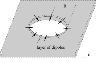
FIG. 4.: Superconducting film with circular hole inside acting as lens for a penetrating electron beam.

So far we have derived that the surface of a high–$T_{\rm c}$ superconductor can induce a charge modulation. Now we comment on a possible experimental observation of this effect. One setup, an “electrooptical lens”, is shown in Fig. 4 and can be considered as idealization of a recent experiment [6]. Motivated by the observed lens effect, which sets in when the material becomes superconducting, we will examine to what extent it can be ascribed to a surface charging according to the presented mechanism.

Let us assume that the sample is a thin $d$-wave superconducting monocrystalline film with a micro-size circular hole inside. The surfaces of the film are assumed to be smooth and parallel to the $XY$ crystal plane. Assuming specular reflection, the order parameter is not suppressed at these surfaces according to Eq. (26). But the inner surface of the hole is normal to the $XY$ plane leading to a strongly suppressed gap function at the boundary of the hole. Due to the preparation of the hole this surface should be rough leading to a decrease of the order parameter around the hole according to Eq. (22). Thus one obtains a charge accumulation around the hole only [15]. Since the real charge distribution consists of two layers of positive and negative charge one can think of this distribution as a ring of dipoles oriented normal to the boundary of the hole, see Fig. 4. The corresponding electrostatic field should be observable in different ways. One possible way to detect the ring of dipoles is to send a very slow and weak beam of electrons through the hole. The intensity in the center of the beam image behind the hole then changes when the sample is cooled below $T_{\rm c}$ due to the (de)focusing caused by the accumulated dipoles.

In the actual experiment by Kriebel et al. [6] a similar geometry was examined by transmission electron microscopy. They have observed a very small change in the image intensity of the electron beam at the superconducting transition. However, the actual sample was polycrystalline and can not be expected to lead to such a well-defined field distribution as in our ideal situation described above. Nevertheless, to obtain the order of magnitude of this lens effect, it is sufficient to consider the simplified setup.

The calculation of the lens effect amounts to solving the electrostatic potential problem for the ring of dipoles. From the electric field we calculate the optical effect in an eikonal approximation for the electrons.

Since we can assume that the radius of the hole is much larger than the correlation length $\xi$, the curvature of the boundary can be neglected. Therefore the accumulated charge can be approximated by the charge density (35) obtained for a plane surface. With the (constant) dipole moment $g$ per unit area from Eq. (37) the electric potential outside the superconducting film is given by

$$\phi({\bf r})=\frac{g}{4\pi}\int_{\rm ring}{\bf n}\cdot{\mathchoice{{\hbox{\boldmath$\displaystyle\nabla$}}}{{\hbox{\boldmath$\textstyle\nabla$}}}{{\hbox{\boldmath$\scriptstyle\nabla$}}}{{\hbox{\boldmath$\scriptscriptstyle\nabla$}}}}\left(\frac{1}{|{\bf r}-{\bf r^{\prime}}|}\right)dS^{\prime}$$ (38)

with the surface normal vector ${\bf n}$ lying in the $XY$ plane and the surface element $dS^{\prime}$ of the ring. For a cylinder with radius $R$ and height $d\ll R$ this leads to

$$\phi(\rho,z)=\frac{gd}{4\pi}\int_{0}^{2\pi}d\varphi\frac{R\rho\cos\varphi-R^{2}}{\left[\rho^{2}+z^{2}+R^{2}-2R\rho\cos\varphi\right]^{3/2}}.$$ (39)

This integral can be expressed in terms of complete elliptic integrals. But we are only interested in the radial electric field component averaged along the $z$ direction to obtain the total intensity change. Let us assume that an electron moves initially at a radial distance $\rho_{i}$ from the center in the negative $z$-direction with vanishing radial velocity. To minimize the influence of the source of the electron on the effect one should assume that the source is asymptotically far away.

For this radial distance $\rho_{i}$ from the $z$-axis the averaged value of the deflecting field for $-L<z<0$, defined by

$$\overline{E_{\rho}}(\rho_{i})=\frac{1}{L}\int_{-L}^{0}dzE_{\rho}(\rho_{i},z),$$ (40)

can be calculated as follows: Consider a virtual cylinder of radius $\rho_{i}$ around the $z$-axis with its ends at $z=0$ and $z=-L$, respectively. For symmetry reasons the flux of the electric field across the abutting face at $z=0$ vanishes. If the lower face of the cylinder is far away from the dipoles, i.e. $L\gg R$, the electric potential at the lower face can be approximated by an asymptotical expansion of (39) in $z$. Then the angular integration is trivial and one obtains for the $z$-component of the asymptotic electric field

$$E_{z}(\rho,z)=\frac{3gdR^{2}}{4}\frac{2z^{2}-10\rho^{2}-5R^{2}}{z^{6}}+{\mathcal{O}}(z^{-8}).$$ (41)

Because there is no charge located inside the virtual cylinder, the total flux of the electric field across the surface of the cylinder vanishes. Using the asymptotic value (41) to calculate the flux across the face at $z=-L$ one obtains the averaged radial field for $z<0$

$$\overline{E_{\rho}}(\rho_{i})\approx\frac{3}{8}gd\rho_{i}R^{2}\frac{5(\rho_{i}^{2}+R^{2})-2L^{2}}{L^{7}}.$$ (42)

For symmetry reasons the same expression holds for an average of the electric field in the upper half space. We take $L\rightarrow\infty$ as starting position of the electrons. Therefore the electric field in the upper half space does not contribute to the total deflection of the electron, as can be seen easily from (42). Since the whole change in the intensity comes then from the path of the electron behind the film, the optimal position $z=-L$ of the detector has to be obtained by a maximization of the averaged radial field (42) as a function of $L$. For electrons near by the center of the hole ($\rho_{i}\approx 0$) the optimal distance is $L=(\sqrt{14}/2)R$. For this rather small value of $L$ it can be checked numerically that the asymptotic approximation used for the average procedure underestimates $\overline{E_{\rho}}$ only by a factor $\approx 2$ if $\rho_{i}\ll R$. Using this optimized value, the electron will be detected at $z=-L$ with a radial distance $\rho_{f}(\rho_{i})$ from the center given by

$$\rho_{f}(\rho_{i})=\rho_{i}(1-\alpha_{0}+\alpha_{2}\rho_{i}^{2})$$ (43)

with

$$\alpha_{0}\approx 0.016\frac{e}{m}\frac{gd}{Rv_{0}^{2}},$$ (44)

$$\alpha_{2}\approx 0.04\frac{e}{m}\frac{gd}{R^{3}v_{0}^{2}},$$ (45)

where $v_{0}$ is averaged velocity of the electron with respect to the $z$ direction. The relative enhancement of the intensity at the center is then given by

$$\left.\frac{d\rho_{i}}{d\rho_{f}}\right|_{\rho_{f}=0}=\frac{1}{1-\alpha_{0}}.$$ (46)

Using the density of the dipole moment (37) we obtain for the deflection parameter

$$\alpha_{0}\approx-3.2\cdot 10^{-3}\frac{e^{2}a_{\rm B}}{mv_{0}^{2}\xi^{2}}\frac{d}{R}\approx-\frac{10^{-4}{\rm eV}}{E_{\rm kin}}\frac{d}{R},$$ (47)

where we have used $\xi\approx 10$Å as a typical value for high–$T_{\rm c}$ superconductors in the last expression. The spatial variation of the relative intensity $I(\rho_{f})=d\rho_{i}/d\rho_{f}$ determined by (43) is shown in Fig. 5. Strictly, the shown numerical result is valid only for distances $\rho_{f}\ll R$ due to the truncation of higher order terms of $\rho_{i}$ in Eq. (43).

FIG. 5.: Variation of the relative intensity $I(\rho_{f})$ of the electron beam image across the hole behind the superconducting film.

V Discussion

In Sec. II we have presented an explicit microscopic calculation of the extrapolation length in $d$-wave superconductors. Within the quasiclassical approximation we found $b\sim\xi_{0}$, which is of the order of 12Å in YBCO. Within the same approximation microscopic calculations[16] for $s$-wave superconductors give $b=\infty$, i.e. no suppression of the order parameter at the surface. In the $s$-wave case a finite value of

$$b\sim\xi_{0}^{2}/a$$ (48)

can be found only if one goes beyond the quasiclassical approximation, taking special care of the finite thickness of the metal-vacuum transition layer[17, 16]. From this expression one can expect small $b$, i.e. a notable suppression of the condensate near the surface, if $\xi_{0}$ is small (i.e. of the order of $a$). This is the case for HTSC as has been pointed out by Deutscher and Müller[18]. However, Eq. (48) is based on approximations which are valid only as long as $b\gg\xi_{0}$. For $d$-wave superconductivity the situation is very different: as our calculation shows, the most important reason for the reduction of $b$ is the $d$-wave symmetry itself. In this case the effect is so pronounced that it can be obtained within the quasiclassical approximation.

It should be emphasized that in this article we assume the superconducting order parameter to have the pure $d_{x^{2}-y^{2}}$-symmetry [see Eq. (2)], which immediately follows from the chosen form of the pairing potential (A3) containing the spherical harmonics corresponding only to the irreducible representation $B_{1g}$ of the tetragonal group. In general, one could allow for the possibility of a small admixture of the $s$-wave component. As shown in Ref. [19], such an admixture appears whenever one deals with a spatially non-uniform distribution of the order parameter, e.g. near surfaces, twinning planes, columnar defects etc. and is brought about by the presence of the mixed-gradient terms in the GL expansion of the free energy. In our work we neglect this effect due to the results of Ref. [19]: (i) The induced $s$-wave component is always much smaller (by one order of magnitude at least) than the $d$-wave one. This holds in particular at temperatures close to $T_{\rm c}$, since the $s$-wave component vanishes faster with $(T_{\rm c}-T)$ than the $d$-wave component. (ii) The $s$-wave component vanishes at the surface together with the $d$-wave component, so that the modulation of $\rho(x)$ shown in Fig. 3 remains unaffected.

The fact, that the $d$-wave order parameter is strongly suppressed at diffusively reflecting superconductor/insulator interfaces, could explain an anomalously weak temperature dependence of the Josephson critical current $j_{\rm c}\sim(T_{\rm c}-T)^{2}$ near $T_{\rm c}$, as observed in Ref. [20]. Indeed, the critical current is proportional to the square of the order parameter at the surface: $j_{\rm c}\sim\Delta^{2}|_{\rm S}$. However, as it follows from our results [see Eq. (27)]: $\Delta|_{\rm S}\sim(b/\xi(T))\Delta_{0}\sim(\xi_{0}/\xi(T))\Delta_{0}$. Hence

$$j_{\rm c}\sim\Delta_{0}^{2}(T)\frac{\xi_{0}^{2}}{\xi^{2}(T)}\sim(T_{\rm c}-T)^{2}$$ (49)

for all orientations, instead of $j_{\rm c}\sim T_{\rm c}-T$, as expected for a conventional SIS junction. The same result has been obtained in [21] for distinguished orientations of a specularly reflecting interface (see also the discussion in the end of Sec. II).

In the present analysis we have neglected possible anisotropy of the Fermi surface, which is characteristic for HTSC. In terms of the ratio of effective masses in a Ginzburg-Landau theory this anisotropy can be of the order $m_{\perp}/m_{\parallel}\sim 100$. The generalization of our analysis to anisotropic Fermi surfaces is straightforward but rapidly leads to cumbersome analytic expressions. Such a generalization has been performed by Shapoval [22] for the case of an anisotropic $s$-wave pairing. For $d$-wave pairing we expect that this generalization leads only to quantitative changes which only weakly affect the boundary condition $b\ll\xi(T)$. Although $N_{0}^{\prime}$ and $\lambda_{\rm TF}\sim N_{0}^{-1/2}$ drastically depend on the mass anisotropy. In contrast the combination $N_{0}^{\prime}\lambda_{\rm TF}^{2}$ is insensitive. Therefore only the spatial distribution of charge $\varrho$ will be affected, but not the total charge $Q$ or the dipole moment $g$.

The amplitude of the electrooptical lens effect, Eq. (47), crucially depends on the beam energy of the electrons. In the experiment of Ref. [6] a beam energy of $E_{\rm kin}=120$keV was used, which leads to $\alpha_{0}\sim 10^{-9}$ at the optimum distance $L\sim R$ behind the lens. However, the actual picture was generated much further away, where the intensity rapidly decreases according to Eq. (42). In addition, the sample had a much more irregular shape than in our idealized geometry. We expect this irregularity to reduce the electrooptical effect of the dipole layer. Therefore we believe that surface charging has to be excluded as the origin of the lens effect with $\alpha_{0}\sim 10^{-2}$ observed in this particular experiment.

At present, the actual origin for the observed effect can not be deduced unambiguously from the experiment. One contribution could be due to a charge accumulation at the surface of the superconductor which is directly hit by the electron beam. The amount of accumulated charge then strongly depends on the conductivity of the sample which drastically changes at $T_{\rm c}$. Since in the experiment polycrystalline samples have been used, there are small magnetic fields induced by the Josephson currents between the grains. But these fields should give an even weaker deflection of the electrons since the local field sources do not sum up constructively.

In order to clarify this situation it would be desirable to use lower electron energies where the the electrooptical effect should become stronger. For $E_{\rm kin}=100$eV as used in LEED, $\alpha_{0}\sim 10^{-6}$ can be achieved due to surface charging at the optimum distance. In addition, the use of a single crystalline sample with a more regular shape of the hole would be desirable as well as a spatial resolution of the density profile.

Finally, to detect the charging effect, other experimental techniques might be more promising than the lens effect examined above. For example, the local stray field outside the superconductor may be probed by atomic force microscopy, as already suggested by Blatter et al. [4] for vortices.

A d-wave pairing

We briefly point out the most important changes for $d_{x^{2}-y^{2}}$-pairing in contrast to conventional $s$-wave pairing in a weak-coupling BCS model. A discussion of arbitrary symmetry has been summarized in Ref. [10]. For calculational convenience we ignore mass anisotropy and use a dispersion relation $\epsilon_{\bf k}=k^{2}/2m-\mu$ of single electron states. They have a density of states (per spin projection)

$$N_{\epsilon}:=\int\frac{d^{3}k}{(2\pi)^{3}}\delta(\epsilon-\epsilon_{\bf k})=\frac{[2m^{3}(\epsilon+\mu)]^{1/2}}{2\pi^{2}}.$$ (A1)

Irrespective of specific pairing mechanism, the gap function for singlet Cooper pairs with relative momentum ${\bf k}$ can be written as

$$\Delta_{{\bf k},\alpha\beta}=(i\sigma_{y})_{\alpha\beta}\psi({\bf k})\Delta_{0}=\int\frac{d^{3}k^{\prime}}{(2\pi)^{3}}V({\bf k},{\bf k}^{\prime})\langle a_{{\bf k}^{\prime}\alpha}a_{-{\bf k}^{\prime}\beta}\rangle.$$ (A2)

For a singlet state the potential can be approximated by

$$V({\bf k},{\bf k}^{\prime})=\left\{\begin{array}[]{ll}-V\psi({\bf k})\psi^{*}({\bf k}^{\prime}),&|\epsilon_{\bf k}|,|\epsilon_{{\bf k}^{\prime}}|\leq\epsilon_{\rm c}\\ 0,&{\rm otherwise}\end{array}\right.$$ (A3)

with an energy cutoff $\epsilon_{\rm c}$ of the interaction. For anisotropic masses the definition (2) of $\psi$ was normalized such that $\langle\psi^{2}({\bf k})\rangle_{0}=1$ with an average

$$\langle(\dots)\rangle_{0}=\frac{1}{N_{0}}\int\frac{d^{3}k}{(2\pi)^{3}}\delta(\epsilon_{\bf k})(\dots)$$ (A4)

defined on the Fermi surface.

In the BCS mean-field (MF) approximation the Hamiltonian is diagonalized by the Bogoliubov transformation with parameters

$$|u_{\bf k}|^{2} = (1+\epsilon_{\bf k}/E_{\bf k})/2$$ (A5)

$$|v_{\bf k}|^{2} = (1-\epsilon_{\bf k}/E_{\bf k})/2$$ (A6)

$$E_{\bf k} = \sqrt{\epsilon_{\bf k}^{2}+|\Delta_{0}|^{2}\psi^{2}({\bf k})}$$ (A7)

The self-consistency equation for the MF approximation reads

$$1=V\int^{\prime}\frac{d^{3}k}{(2\pi)^{3}}|\psi({\bf k})|^{2}\frac{1-2f(E_{\bf k})}{2E_{\bf k}}$$ (A8)

with the Fermi-Dirac distribution function $f(E)=1/[1+\exp(E/T)]$. The primed integral runs over ${\bf k}$ with $|\epsilon_{\bf k}|<\epsilon_{\rm c}$ only.

For $\Delta_{0}\to 0$ Eq. (A8) implicitly determines

$$T_{\rm c}=1.14\ \epsilon_{\rm c}\exp(-1/VN_{0}).$$ (A9)

Due to the choice of the normalization of $\psi$, this relation does not depend explicitly on pairing symmetry or mass anisotropy.

In the critical region the amplitude of the gap follows from Eq. (A8) after expansion in second order of $\Delta_{0}$ and linearizing in $1-T/T_{\rm c}$:

$$|\Delta_{0}(T)|^{2}=\langle\psi^{4}\rangle_{0}^{-1}\frac{8\pi^{2}}{7\zeta(3)}(1-T/T_{\rm c})\ T_{\rm c}^{2}.$$ (A10)

In comparison to the isotropic $s$-wave case this result is modified by a factor $\langle\psi^{4}\rangle_{0}=15/7$.

We now calculate for fixed electrochemical potential the change in electron density due to formation of a gap. In the superconducting state a single electron state ${\bf k}$ has occupation number

$$n^{\rm s}_{\bf k}=|v_{\bf k}|^{2}+(|u_{\bf k}|^{2}-|v_{\bf k}|^{2})f(E_{\bf k})$$ (A11)

compared to the normal state with $n^{\rm n}_{\bf k}=f(\epsilon_{\bf k})$. The change of the total electron density

$$\delta n=2\int^{\prime}\frac{d^{3}k}{(2\pi)^{3}}\left(n^{\rm s}_{\bf k}-n^{\rm n}_{\bf k}\right)$$ (A12)

can be evaluated using the Sommerfeld approximation $N_{\epsilon}\approx N_{0}+\epsilon N^{\prime}_{0}$. One finds to lowest order in $\Delta_{0}$, i.e. close to $T_{\rm c}$,

$$\delta n\approx N^{\prime}_{0}|\Delta_{0}|^{2}\ln\frac{\epsilon_{\rm c}}{T_{\rm c}},$$ (A13)

where again all dependence on pairing symmetry and mass anisotropy is contained in $T_{\rm c}$. Since the condensate density $|\Delta_{0}|^{2}$ has a discontinuous slope near $T_{\rm c}$, Eq. (A13) implies that for fixed electrochemical potential the electron density has a discontinuous slope or, vice versa, the chemical potential for fixed electron density. This effect and its consequences for the work function has been pointed out by van der Marel[5].

B Method of classical trajectories

As shown in Ref. [10], the kernel $K$ in Eq. (5) is determined by the following expression, which is valid for arbitrary symmetry of the order parameter:

$$K({\bf r}_{1},{\bf r}_{2}) = \pi VN_{0}T\sum_{n}\int_{0}^{\infty}dt~{}\exp(-2|\omega_{n}|t)$$ (B2)

$$\times\left\langle\psi^{*}({\bf n}_{1})\psi({\bf n}_{2})\right\rangle_{\epsilon=0,{\rm classical}},$$

where $t>0$ is the time of motion along the trajectory and $\omega_{n}=(2n+1)\pi T$ is a Matsubara frequency. The angular brackets denote the averaging over all possible classical trajectories ${\bf r}(t)$ of a particle, moving with the Fermi velocity $v_{F}$, which connect the points ${\bf r}_{1}$ and ${\bf r}_{2}$ and satisfy the condition ${\bf r}(0)={\bf r}_{1}$ (one has to take into account both the trajectories, for which ${\bf r}(t)={\bf r}_{2}$, and the time-reversed trajectories, which give just a Hermitian-conjugated contribution to the kernel). The unit vectors ${\bf n}_{1}$ and ${\bf n}_{2}$ denote the directions of velocity in the corresponding points. We shall keep below the general notations for the basis functions (which are chosen to be real), so that our results are applicable for any one-dimensional spin-singlet order parameter.

Let us first consider the contribution from straight trajectories. The expression in the angular brackets in the r.h.s. of (B2) has the form:

$$\langle(...)\rangle_{\rm direct}=\int\frac{d\Omega}{4\pi}~{}\delta({\bf r}_{2}-{\bf r}(t))\psi^{2}({\bf n})+{\rm h.c.},$$ (B3)

where ${\bf r}(t)={\bf r}_{1}+v_{F}{\bf n}t$ is the only straight path from ${\bf r}_{1}$ to ${\bf r}_{2}$ (see Fig. 1a, ${\bf n}_{1}={\bf n}_{2}={\bf n}$). Here, integration is over all directions of ${\bf n}$. Hence

$$K_{0}({\bf r}_{1}-{\bf r}_{2})=K_{0}({\bf r})=\frac{VN_{0}}{4\pi\xi_{0}}\frac{\psi^{2}({\bf n})}{r^{2}\sinh(r/\xi_{0})}$$ (B4)

with $\xi_{0}=v_{\rm F}/2\pi T_{\rm c}$, and ${\bf n}={\bf r}/|{\bf r}|$. In the critical region the correlation lengths $\xi_{i}$ along different directions are given by

$$\xi^{2}_{i}(T)=\gamma_{i}\frac{7\zeta(3)}{12}\left(1-\frac{T}{T_{\rm c}}\right)^{-1}\xi_{0}^{2}.$$ (B5)

Due to the $d$-wave pairing, there is an anisotropy (even for the spherical Fermi surface) described by the factors $\gamma_{X}=\gamma_{Y}=9/7$ and $\gamma_{Z}=3/7$.

The equation (6) follows from (5) as a result of integration over the differences $y_{2}-y_{1}$ and $z_{2}-z_{1}$:

$$\Delta(x_{1})=\int_{0}^{\infty}dx_{2}~{}K(x_{1},x_{2})\Delta(x_{2}),$$ (B6)

the kernel being given by the sum of two terms:

$$K(x_{1},x_{2})=K_{0}(x_{1}-x_{2})+K_{\rm r}(x_{1},x_{2}),$$ (B7)

where the contributions $K_{0}$ and $K_{\rm r}$ come respectively from the straight trajectories and those ones, which are reflected against the surface.

Substituting (B3) in Eq. (B2), we obtain:

$$K_{0}(x)=\frac{VN_{0}}{2\xi_{0}}\sum_{n}\int_{0}^{1}\frac{ds}{s}~{}F_{0}(s)\exp\left(-\frac{2|\omega_{n}|}{v_{F}s}|x|\right),$$ (B8)

where

$$F_{0}(s)=\int_{0}^{2\pi}\frac{d\varphi}{4\pi}~{}\Bigl{[}\psi^{2}(s,\varphi)+\psi^{2}(-s,\varphi)\Bigr{]}.$$ (B9)

Here $s=\cos\theta$, $\theta$ and $\varphi$ are the polar and azimuthal angles respectively, so that ${\bf n}=(s,\sqrt{1-s^{2}}\cos\varphi,\sqrt{1-s^{2}}\sin\varphi)$. The polar axis is chosen along the normal vector to the surface (Fig. 1). Note that $\int_{0}^{1}dsF_{0}(s)=1$ because of the normalization condition of the basis functions.

The form of $K_{\rm r}(x_{1},x_{2})$ is determined by the reflection of electrons at the boundary. For the case of specularly reflecting boundary we have from (B2) the following expression:

$$\langle(...)\rangle_{\rm reflected}=\int\frac{d\Omega}{4\pi}~{}\delta({\bf r}_{2}-{\bf r}(t))\psi({\bf n}_{1})\psi({\bf n}_{2})+{\rm h.c.}$$

The only possible reflected path is (see Fig. 1b):

$${\bf r}(t)=\left\{\begin{array}[]{ll}{\bf r}_{1}+v_{F}{\bf n}_{1}t&\quad,\quad t<t_{0}=-\frac{x_{1}}{v_{F}s_{1}}~{},\\ v_{F}{\bf n}_{2}(t-t_{0})&\quad,\quad t>t_{0}~{},\end{array}\right.$$ (B10)

where $t_{0}$ corresponds to the moment when the particle hits the surface and ${\bf n}_{1,2}=(\pm s,\sqrt{1-s^{2}}\cos\varphi,\sqrt{1-s^{2}}\sin\varphi)$ ($s_{1}<0$). Performing integrations we obtain:

$$K_{\rm r}(x_{1},x_{2})=\frac{VN_{0}}{2\xi_{0}}\sum_{n}\int_{0}^{1}\frac{ds}{s}~{}F_{\rm r}(s)$$ (B11)

$$\times\exp\left(-\frac{2|\omega_{n}|}{v_{F}s}(x_{1}+x_{2})\right),$$ (B12)

where

$$F_{\rm r}(s)=\int_{0}^{2\pi}\frac{d\varphi}{2\pi}~{}\psi(s,\varphi)\psi(-s,\varphi).$$ (B13)

The results (B9) and (B13) obviously coincide with those obtained in Ref.[12] by another method.

In the case of diffusive surface one needs to take into account all possible trajectories, reflected in all directions (see Fig. 1c):

$$\langle(...)\rangle_{\rm reflected}=\int\frac{d\Omega_{1}}{4\pi}\int d\Omega_{2}~{}P({\bf n}_{1},{\bf n}_{2})~{}\delta({\bf r}_{2}-{\bf r}(t))$$

$$\times\psi({\bf n}_{1})\psi({\bf n}_{2})+{\rm h.c.},$$

where $P({\bf n}_{1},{\bf n}_{2})$ is the probability distribution for the particle to be reflected in the direction ${\bf n}_{2}$, provided it moved before along the direction ${\bf n}_{1}$. Assuming the reflection is completely diffusive (i.e. the ”memory” is completely lost), we obtain that this probability density depends only on ${\bf n}_{2}$. As usual, it is convenient to choose it in the following manner: $P({\bf n}_{2})=\frac{1}{\pi}\cos\theta_{2}=\frac{1}{\pi}s_{2}$. The corresponding trajectories are given by (B10), where ${\bf n}_{1}$ and ${\bf n}_{2}$ are now independent unit vectors. After integrations, the resulting expression for $K_{\rm r}$ is [13]:

$$K_{\rm r}(x_{1},x_{2})=\frac{VN_{0}}{2\xi_{0}}\sum_{n}\int_{0}^{1}ds_{1}\int_{0}^{1}ds_{2}~{}F_{\rm r}(s_{1},s_{2})$$ (B14)

$$\times\exp\left(-\frac{2|\omega_{n}|}{v_{F}}\left(\frac{x_{1}}{s_{1}}+\frac{x_{2}}{s_{2}}\right)\right),$$ (B15)

where

$$F_{\rm r}(s_{1},s_{2})=\int\limits_{0}^{2\pi}\frac{d\varphi_{1}}{2\pi}\int\limits_{0}^{2\pi}\frac{d\varphi_{2}}{2\pi}\Bigl{[}\psi(s_{1},\varphi_{1})\psi(-s_{2},\varphi_{2})$$ (B16)

$$+\psi(-s_{1},\varphi_{1})\psi(s_{2},\varphi_{2})\Bigr{]}.$$ (B17)

Using the specific angular dependence (2) of the order parameter, the general expressions (B9) and (B16) lead to Eqs. (9) and (11).

Note that if the contribution from the diffusively reflected trajectories vanishes then the integral equation (6) can be solved exactly using the Wiener-Hopf method. This takes place for any spin-triplet order parameter, in particular for $p$-wave order parameter in the superfluid phases of ³He [23].

REFERENCES

-
[1]
Present address: Theory of Condensed Matter Group,
Cavendish Laboratory, University of Cambridge, Madingley Road,
Cambridge CB3 0HE, UK.
Permanent address: L. D. Landau Institute for Theoretical Physics, Kosygina Str. 2, 117940 Moscow, Russia.
- [2] D.I. Khomskii and F.V. Kusmartsev, Pis’ma v Zh. Eksp. Teor. Fiz. 54, 150 (1991) [JETP Lett. 54, 145 (1991)]; Phys. Rev. B 46, 14245 (1992).
- [3] D.I. Khomskii and A. Freimuth, Phys. Rev. Lett. 75, 1384 (1995).
- [4] G. Blatter, M. Feigel’man, V. Geshkenbein, A. Larkin, and A. van Otterlo, Phys. Rev. Lett. 77, 566 (1996).
- [5] D. van der Marel, Physica C 165, 35 (1990); G. Rietveld, N.Y. Chen, and D. van der Marel, Phys. Rev. Lett. 69, 2578 (1992).
- [6] Cl. Kriebel et al, Ann. d. Phys. 4, 136 (1995).
- [7] see, e.g., J. Annett, N. Goldenfeld, and A.J. Leggett, in Physical Properties of High-Temperature Superconductors, Vol. 5, ed. D.M. Ginsberg (World Scientific, Singapore, 1996).
- [8] G.E. Volovik, Pis’ma v Zh. Eksp. Teor. Fiz. 58, 457 (1993) [JETP Letters 58, 469 (1993)]; P.I. Soininen, C. Kallin, and A.J. Berlinsky, Phys. Rev. B 50, 13883 (1994); R. Heeb, A. van Otterlo, M. Sigrist, and G. Blatter, Phys. Rev. B 54, 9385 (1996).
- [9] see, e.g., P.G. de Gennes, Superconductivity of Metals and Alloys (Benjamin, New York, 1966).
- [10] M. Sigrist and K. Ueda, Rev. Mod. Phys. 63, 239 (1991).
- [11] G. Lüders and K.D. Usadel, The Method of the Correlation Function in the Superconductivity Theory (Springer, Berlin, 1971).
- [12] K.V. Samokhin, Zh. Eksp. Teor. Fiz. 107, 906 (1995) [JETP 80, 515 (1995)].
- [13] K.V. Samokhin, Ph.D. Thesis, L.D. Landau Institute (1995), unpublished.
- [14] D.F. Agterberg and M.B. Walker, Phys. Rev. B 53, 15201 (1996).
- [15] Even if one considers diffusively reflecting surfaces at the top and the bottom of the film, the dipole moments are small compared to the inner surface since . In addition, the dipole moments at the top and at the bottom have opposite orientation and therefore give a negligible contribution to the lens effect.
- [16] P.G. de Gennes, Rev. Mod. Phys. 36, 225 (1964).
- [17] C. Caroli, P.G. de Gennes, and J. Matricon, J. Phys. Rad. 23, 707 (1962); see also Ref. [9] p. 229.
- [18] G. Deutscher and K.A. Müller, Phys. Rev. Lett. 59, 1745 (1987).
- [19] J.-H. Xu, Y. Ren and C.S. Ting, Phys. Rev. B 52, 7663 (1995); J.J. Vicente Alvarez, G.C. Buscaglia and C.A. Balseiro, Phys. Rev. B 54, 16168 (1996)
- [20] R. Gross et al, Phys. Rev. Lett. 64, 228 (1990)
- [21] Yu.S. Barash, A.V. Galaktionov and A.D. Zaikin, Phys. Rev. B 52, 665 (1995)
- [22] E.A. Shapoval, Zh. Eksp. Teor. Fiz. 88, 1073 (1985) [Sov. Phys. JETP 61, 630 (1985)]
- [23] V. Ambegaokar, P.G. de Gennes and D. Rainer, Phys. Rev. A 9, 2676 (1974).