The NMR relaxation rate of ¹⁷O in Sr₂CuO₂Cl₂: Probing two-dimensional magnons at short distances

Abstract

We calculate the nuclear relaxation rate $1/T^{\rm O}_{1}$ of oxygen in the undoped quasi two-dimensional quantum Heisenberg antiferromagnet Sr₂CuO₂Cl₂ above the Neel temperature. The calculation is performed at two-loop order with the help of the Dyson-Maleev formulation of the spin-wave expansion, taking all scattering processes involving two and three magnons into account. At low temperatures $T$ we find $1/T^{\rm O}_{1}=c_{1}T^{3}+c_{2}T^{4}+O(T^{5})$, and give explicit expressions for the coefficients $c_{1}$ (two-magnon scattering) and $c_{2}$ (three magnon scattering). We compare our result with a recent experiment by Thurber et al. and show that this experiment directly probes the existence of short-wavelength magnons in a two-dimensional antiferromagnet.

I Introduction

In a recent experiment[1] Thurber et al. reported nuclear magnetic resonance (NMR) measurements of the ¹⁷O and ⁶³Cu relaxation rates of the undoped and lightly doped quasi two-dimensional quantum Heisenberg antiferromagnet Sr₂CuO₂Cl₂. In this compound the anisotropies and inter-layer couplings are particularly weak, so that in the undoped case it is an excellent approximation to model the dynamics of the localized $S=1/2$ spins at the Cu sites above the Neel temperature $T_{N}$ by an isotropic two-dimensional nearest neighbor quantum Heisenberg antiferromagnet. The Hamiltonian is given by

$$\hat{H}=J\sum_{{\bf{r}}}\sum_{i=x,y}{\bf{S}}_{\bf{r}}\cdot{\bf{S}}_{{\bf{r}}+{\bf{a}}_{i}}\;\;\;,$$ (1)

where the ${\bf{r}}$-sum is over the $N$ sites of the square lattice formed by the Cu-sites, and ${\bf{a}}_{x}$ and ${\bf{a}}_{y}$ are the primitive lattice vectors with length $|{\bf{a}}_{i}|=a$. The operators ${\bf{S}}_{\bf{r}}$ are $SU(2)$ spin operators satisfying ${\bf{S}}_{\bf{r}}^{2}=S(S+1)$, and $J>0$ is the antiferromagnetic exchange coupling. NMR experiments measure the relaxation of the nuclear spins due to their coupling to the reservoir of the electronic spin lattice. The theoretical framework for the calculation of the NMR rates in Heisenberg antiferromagnets has been discussed 30 years ago by Beemann and Pincus[2], and more recently for two-dimensional antiferromagnets in Refs.[3, 4, 5, 6]. However, so far only the leading order of the low-temperature behavior has been calculated, which is determined by two-magnon scattering and can be obtained from a simple one-loop calculation. For a quantitative comparison with the experimental result[1] for the NMR rate of ¹⁷O it is important to know also the contribution from three-magnon scattering, which describes the leading effect of magnon-magnon interactions. In this work we shall explicitly calculate this correction and compare it with the experiment of Thurber et al.[1].

To begin with, let us briefly derive the NMR rate from Fermi’s golden rule. Note that Mila and Rice[4] gave the relevant form factor only up to a constant of proportionality. However, for a quantitative comparison with experiments we need to know the precise numerical value of the form factor. In the simplest approximation, the coupling between the nucleus and the electronic spins can be described by an isotropic hyperfine interaction[2, 3, 4, 5, 6]. For a nuclear spin ${\bf{I}}^{\rm Cu}_{\bf{R}}$ of ⁶³Cu at position ${\bf{R}}$ this is of the form $\hat{H}^{\rm Cu}=A_{\rm Cu}{\bf{I}}^{\rm Cu}_{\bf{R}}\cdot{\bf{S}}_{{\bf{R}}}$, with some characteristic energy scale $A_{\rm Cu}$ that can be obtained from experiments. As discussed by Chakravarty and Orbach[5], the ⁶³Cu NMR-rate is dominated by critical antiferromagnetic fluctuations, and cannot be calculated via the perturbative spin-wave expansion. On the other hand, the nuclear spins ${\bf{I}}^{\rm O}_{\bf{R}}$ at the ¹⁷O-site are coupled to the electronic spins of two neighboring Cu sites (see Fig. 1), so that the hyperfine interaction is

$$\hat{H}^{\rm O}=A_{\rm O}{\bf{I}}^{\rm O}_{\bf{R}}\cdot\sum_{i=1,2}{\bf{S}}_{{\bf{R}}+{\bf{b}}_{i}}\;\;\;,$$ (2)

where ${\bf{b}}_{1}=-{\bf{a}}_{x}/2$ and ${\bf{b}}_{2}={\bf{a}}_{x}/2$. Let us emphasize that Eq.(2) involves the average ${\bf{S}}_{{\bf{R}}+{\bf{a}}_{x}/2}+{\bf{S}}_{{\bf{R}}-{\bf{a}}_{x}/2}$ of two neighboring electronic spins. Given the fact that the spins couple antiferromagnetically, it is clear that at least in the classical picture the total spin vanishes. Hence, we expect that the ¹⁷O relaxation rate is dominated by short wavelength antiferromagnetic quantum fluctuations. In this work we shall put this expectation on a solid quantitative basis, and show that the NMR relaxation rate $1/T_{1}^{\rm O}$ at the oxygen site probes the unique short-distance behavior of magnons in two-dimensional Heisenberg magnets.

Keeping in mind that $1/T_{1}$ is defined such that calculations should always use the matrix elements for nuclear spins with magnitude $I=1/2$, straightforward application of Fermi’s golden rule yields for the NMR relaxation rate of ¹⁷O

$$\frac{1}{T_{1}^{\rm O}}=\frac{A_{\rm O}^{2}}{3\hbar^{2}}2\pi\hbar\sum_{\alpha\beta}p_{\alpha}\langle\alpha|\sum_{i}{\bf{S}}_{{\bf{R}}+{\bf{b}}_{i}}|\beta\rangle\cdot\langle\beta|\sum_{j}{\bf{S}}_{{\bf{R}}+{\bf{b}}_{j}}|\alpha\rangle\delta(\hbar\omega_{N}-E_{\alpha}+E_{\beta})\;\;\;,$$ (3)

where $E_{\alpha}$ and $|\alpha\rangle$ are exact eigen-energies and eigen-states of the Heisenberg Hamiltonian (1), and $p_{\alpha}=e^{-E_{\alpha}/T}/Z$, where $Z=\sum_{\alpha}e^{-E_{\alpha}/T}$. Here $T$ is the temperature, measured in units of energy. In experiments the resonance energy $\hbar\omega_{N}$ is usually much smaller than all characteristic energies of the spin system, so that we may set $\omega_{N}=0$. Defining the Fourier transformed spin operators ${\bf{S}}_{\bf{r}}={{N}}^{-1/2}\sum_{\bf{k}}e^{-i{\bf{k}}\cdot{\bf{r}}}{\bf{S}}_{\bf{k}}$, where the ${\bf{k}}$-sum is over the first Brillouin zone of the reciprocal lattice, we obtain from Eq.(3) for $\omega_{N}\rightarrow 0$

$$\frac{1}{T_{1}^{\rm O}}=\frac{A_{\rm O}^{2}}{3\hbar^{2}N}\sum_{\bf{k}}f({\bf{k}})S({\bf{k}},0)\;\;\;,$$ (4)

where $S({\bf{k}},\omega)$ is the dynamic structure factor of the Cu-spin lattice,

$$S({\bf{k}},\omega)=2\pi\hbar\sum_{\alpha\beta}p_{\alpha}\langle\alpha|{\bf{S}}_{\bf{k}}|\beta\rangle\cdot\langle\beta|{\bf{S}}_{-\bf{k}}|\alpha\rangle\delta(\hbar\omega-E_{\alpha}+E_{\beta})\;\;\;,$$ (5)

and the form factor is[7]

$$f({\bf{k}})=2\left[1+\cos(k_{x}a)\right]\;\;\;.$$ (6)

Note that a transition between the two states of the nuclear spin is described by the ladder operators $I^{\pm}=I^{x}\pm iI^{y}$, which couple to the transverse components $S^{\mp}=S^{x}\mp iS^{y}$ of the electronic spins. However, for temperatures above the Neel temperature the system is rotationally invariant in spin space, which enables us to express the NMR rate in terms of the rotationally invariant dynamic structure factor (5). This is a very important point, because we would like to calculate the dynamic structure factor in Eq.(4) by means of the spin-wave expansion. At the first sight it seems that for two-dimensional Heisenberg magnets at finite temperatures this approach cannot be justified, because the naive spin-wave expansion is based on the assumption of long-range order, which is rigorously known to be absent at any finite temperature[8]. For example, an attempt to calculate the staggered magnetization at $T>0$ via spin-wave theory leads to a infrared divergent integral, signalling the inconsistency of the magnon picture in two dimensions[9]. The important point is, however, that spin-rotationally invariant quantities are free of infrared divergencies, and can be calculated with the help the spin-wave expansion even at finite temperatures. For the classical Heisenberg model this has been proven by David[10], and it is reasonable to assume that it remains true for the quantum model. In this work we shall verify explicitly at two-loop order that in the rotationally invariant dynamic structure factor (5) all infrared divergencies that appear at intermediate stages of the calculation indeed cancel.

II The spin-wave expansion for the ¹⁷O NMR rate

In this section we shall briefly describe our procedure for calculating the dynamic structure factor with the help of the Dyson-Maleev formulation of the spin-wave expansion[11]. As compared with the more common Holstein-Primakoff formalism[12], the Dyson-Maleev spin-boson mapping has the advantage that the boson representation of the Hamiltonian involves only one- and two-body terms, so that beyond the leading order in the spin-wave expansion the number of Feynman diagrams generated with the help of the Dyson-Maleev transformation is smaller than in the case of the Holstein-Primakoff formalism. Thus, for our two-loop calculation of the dynamic structure factor the Dyson-Maleev transformation leads to considerable technical simplifications. Of course, final results for physical quantities should be identical in both formalisms.

As usual, we divide the square lattice into two sublattices, labelled $A$ and $B$, such that the nearest neighbors of any given site belong to the other sublattice. The spherical components of the spin operators on the $A$-sublattice are then represented by canonical boson operators $a_{\bf{r}}$ in the following manner,

$$\begin{array}[]{lcl}S^{+}_{\bf{r}}&=&\sqrt{2S}\left[1-(2S)^{-1}a_{\bf{r}}^{\dagger}a_{\bf{r}}\right]a_{\bf{r}}\\ S^{-}_{\bf{r}}&=&\sqrt{2S}a^{\dagger}_{\bf{r}}\\ S^{z}_{\bf{r}}&=&S-a^{\dagger}_{\bf{r}}a_{\bf{r}}\end{array}\;\;\;,\;\;\;{\bf{r}}\in A\;.$$ (7)

Similarly we write on the $B$-sublattice

$$\begin{array}[]{lcl}S^{+}_{\bf{r}}&=&\sqrt{2S}b^{\dagger}_{\bf{r}}\left[1-(2S)^{-1}b_{\bf{r}}^{\dagger}b_{\bf{r}}\right]\\ S^{-}_{\bf{r}}&=&\sqrt{2S}b_{\bf{r}}\\ S^{z}_{\bf{r}}&=&-S+b^{\dagger}_{\bf{r}}b_{\bf{r}}\end{array}\;\;\;,\;\;\;{\bf{r}}\in B\;,$$ (8)

where $b_{\bf{r}}$ are again canonical boson operators. Because of the two-sublattice structure, it is convenient to Fourier transform on both sublattices separately,

$$a_{\bf{r}}=(N/2)^{-1/2}{\sum_{\bf{q}}}^{\prime}e^{i{\bf{q}}\cdot{\bf{r}}}a_{\bf{q}}\;\;\;,\;\;\;b_{\bf{r}}=(N/2)^{-1/2}{\sum_{\bf{q}}}^{\prime}e^{i{\bf{q}}\cdot{\bf{r}}}b_{\bf{q}}\;\;\;,$$ (9)

where the prime indicates that the wave-vector sums are over the $N/2$ points of the reduced Brillouin zone, with the wave-vectors ${\bf{q}}$ measured with respect to the antiferromagnetic ordering wave-vector ${\bf{\Pi}}=[\pi/a,\pi/a]$ (see Fig.2). Because we would like to express all sums consistently in terms of the wave-vectors of the reduced Brillouin zone, we rewrite Eq.(4) as

$$\frac{1}{T_{1}^{\rm O}}=\frac{A_{\rm X}^{2}}{3\hbar^{2}N}{\sum_{\bf{q}}}^{\prime}\left[f({\bf{q}})S({\bf{q}},0)+f_{\rm st}({\bf{q}}){S}_{\rm st}({\bf{q}},0)\right]\;\;\;,$$ (10)

where ${S}_{\rm st}({\bf{q}},\omega)\equiv S({\bf{\Pi}}+{\bf{q}},\omega)$ is the staggered structure factor, and $f_{\rm st}({\bf{q}})\equiv f({\bf{\Pi}}+{\bf{q}})$ is the corresponding form factor. Below it will become obvious that at low temperatures the inverse thermal de Broglie wavelength acts as an ultraviolet cutoff for the ${\bf{q}}$-sums in Eq.(10). Note that the thermal de Broglie wavelength (divided by $2\pi$) of an isotropic antiferromagnet can be written as

$$\lambda_{\rm th}=\frac{\hbar c}{T}\;\;\;,$$ (11)

where $c$ is the spin-wave velocity. Hence, at low temperatures $\lambda_{\rm th}\gg a$, so that the sums in Eq.(10) are dominated by a small circle in the ${\bf{q}}$-plane with radius $\lambda_{\rm th}^{-1}$ around the origin. Obviously the first term in Eq.(10) represents the contribution from fluctuations of the total magnetization. Because these are not critical fluctuations, we expect that the corresponding contribution can be calculated perturbatively. From Eq.(6) we see that for small ${\bf{q}}$ the form factor for $1/T_{1}^{\rm O}$ can be replaced by

$$f({\bf{q}})=4+O(q_{x}^{2})\;\;\;.$$ (12)

On the other hand, the second term in Eq.(10) represents for $|{\bf{q}}|\ll a^{-1}$ long wavelength critical fluctuations of the staggered magnetization. However, the signature of the critical fluctuations contained in $S_{\rm st}({\bf{q}},0)$ is to a large extent removed by the form factor, which vanishes for small ${\bf{q}}$ as

$$f_{\rm st}({\bf{q}})=(q_{x}a)^{2}+O(q_{x}^{4})\;\;\;.$$ (13)

In fact, we shall show shortly that the contributions of both terms on the right-hand side of Eq.(10) have the same order of magnitude, so that the ¹⁷O relaxation rate is determined both by non-critical fluctuations of the total magnetization and by short wavelength antiferromagnetic fluctuations. In contrast, the corresponding form factor for ⁶³Cu is unity for all wave-vectors[3, 4, 5], so that the rate $1/T_{1}^{\rm Cu}$ is completely dominated by critical antiferromagnetic fluctuations[5].

The spin-wave expansion for the dynamic spin-spin correlation functions has been described in an impressive paper by Harris, Kumar, Halperin and Hohenberg[13], so that we can be rather brief here and refer the reader to Ref.[13] for more details. After substituting the Dyson-Maleev transformation (7,8) for the spin operators into Eq.(1) and Fourier transforming the boson operators as in Eq.(9), the spin Hamiltonian in $D$ dimensions is mapped onto the following boson Hamiltonian

$$\hat{H}\rightarrow-NDJS^{2}+\hat{H}_{\rm DM}^{(2)}+\hat{H}_{\rm DM}^{(4)}\;\;\;,$$ (14)

with

$$\hat{H}_{\rm DM}^{(2)}=2DJS{\sum_{\bf{q}}}^{\prime}\left[a^{\dagger}_{\bf{q}}a_{\bf{q}}+b^{\dagger}_{\bf{q}}b_{\bf{q}}+\gamma_{\bf{q}}(a_{\bf{q}}b_{\bf{q}}+a^{\dagger}_{\bf{q}}b^{\dagger}_{\bf{q}})\right]\;\;\;,$$ (15)

$$\hat{H}_{\rm DM}^{(4)}=-\frac{2DJ}{N}{\sum_{{\bf{1}}\ldots{\bf{4}}}}^{\prime}\delta_{\ast}({\bf{3}}+{\bf{4}}-{\bf{1}}-{\bf{2}})\left[2\gamma_{{\bf{2-4}}}a^{\dagger}_{\bf{1}}a_{\bf{3}}b^{\dagger}_{\bf{4}}b_{\bf{2}}+\gamma_{\bf{2}}a^{\dagger}_{\bf{1}}a_{\bf{3}}a_{\bf{4}}b_{\bf{2}}+\gamma_{\bf{3+4-2}}a^{\dagger}_{\bf{1}}b^{\dagger}_{\bf{3}}b^{\dagger}_{\bf{4}}b_{\bf{2}}\right]\;\;\;,$$ (16)

where ${\bf{1}}$ for ${\bf{q}}_{1}$ (and similarly for the other labels), and we have introduced the standard notation $\gamma_{\bf{q}}=D^{-1}\sum_{i=1}^{D}\cos({\bf{q}}\cdot{\bf{a}}_{i})$. The symbol $\delta_{\ast}({\bf{q}})$ indicates momentum conservation up to a vector of the reciprocal lattice associated with the sublattices[14]. The quadratic part $H_{\rm DM}^{(2)}$ of the Dyson-Maleev Hamiltonian is now diagonalized by means of a Bogoliubov transformation,

$$\left(\begin{array}[]{c}a_{\bf{q}}\\ b^{\dagger}_{\bf{q}}\end{array}\right)=u_{\bf{q}}\left(\begin{array}[]{cc}1&-x_{\bf{q}}\\ -x_{\bf{q}}&1\end{array}\right)\left(\begin{array}[]{c}\alpha_{\bf{q}}\\ \beta_{\bf{q}}^{\dagger}\end{array}\right)\;\;\;,$$ (17)

with

$$u_{\bf{q}}=\sqrt{\frac{1+\epsilon_{\bf{q}}}{2\epsilon_{\bf{q}}}}\;\;\;,\;\;\;x_{\bf{q}}=\sqrt{\frac{1-\epsilon_{\bf{q}}}{1+\epsilon_{\bf{q}}}}\;\;\;,$$ (18)

where $\epsilon_{\bf{q}}=\sqrt{1-\gamma_{\bf{q}}^{2}}$. Then we obtain

$$\hat{H}_{\rm DM}^{(2)}=-2DJS+{\sum_{\bf{q}}}^{\prime}E_{\bf{q}}\left[\alpha^{\dagger}_{\bf{q}}\alpha_{\bf{q}}+\beta_{\bf{q}}\beta^{\dagger}_{\bf{q}}\right]\;\;\;.$$ (19)

Here $E_{\bf{q}}=2DJS\epsilon_{\bf{q}}$ is the free magnon dispersion. Taking into account that the $\beta$-operators in Eq.(19) are anti-normal ordered, we obtain the following $1/S$-correction to the ground-state energy, $\delta E_{0}=-2DJSC$, with $C=1-(2/N){\sum_{\bf{q}}}^{\prime}\epsilon_{\bf{q}}$. The numerical value of $C$ has first been calculated by Anderson [15]. In two dimensions the result is $C=0.158$. In our two-loop calculation presented in Sec.IV we shall simply ignore similar zero-temperature renormalizations, which involve higher powers of $1/S$. Quantum corrections of this type are implicitly taken into account by identifying the spin-wave velocity $c$ and the spin stiffness $\rho_{s}$ in our final result (see Eq.(50) below) with the experimentally measured values. Substituting the Bogoliubov transformation (17) into the quartic part $\hat{H}_{\rm DM}^{(4)}$ we obtain totally $10$ different terms describing scattering of the magnons $\alpha_{\bf{q}}$ and $\beta_{\bf{q}}$ in various combinations. The vertices for these scattering processes have been derived in Ref.[13], and will not be reproduced here. For our two-loop calculation we shall use a particular symmetric parameterization of the Dyson-Maleev vertices given in Ref.[16]. It turns out that the complete interaction part of the Dyson-Maleev Hamiltonian can be parameterized in terms of five different vertices, which can be written as

$$V^{(j)}({\bf{q}},{\bf{k}},{\bf{k}}^{\prime})=\frac{u_{{\bf{k}}+{\bf{q}}}u_{{\bf{k}}^{\prime}-{\bf{q}}}}{u_{\bf{k}}u_{{\bf{k}}^{\prime}}}\tilde{V}^{(j)}({\bf{q}},{\bf{k}},{\bf{k}}^{\prime})\;\;,\;\;j=1,\ldots,5\;\;,$$ (20)

where the rescaled vertices $\tilde{V}^{(j)}$ are non-singular. For our purpose it is sufficient to know the leading behavior of these vertices for small wave-vectors[13, 16, 17],

$$\tilde{V}^{(j)}({\bf{q}},{\bf{k}},{\bf{k}}^{\prime})\sim\left\{\begin{array}[]{ll}\frac{1}{2}(1-\hat{\bf{k}}\cdot\hat{\bf{k}}^{\prime})&\mbox{for $j=1,2,5$}\\ \frac{1}{2}(1+\hat{\bf{k}}\cdot\hat{\bf{k}}^{\prime})&\mbox{for $j=3,4$}\end{array}\right.\;\;\;,$$ (21)

where $\hat{\bf{k}}={\bf{k}}/|{\bf{k}}|$ and $\hat{\bf{k}}^{\prime}={\bf{k}}^{\prime}/|{\bf{k}}^{\prime}|$ are unit vectors.

The boson representations of the spin-spin correlation functions are obtained in a similar manner. To calculate the dynamic structure factor at finite temperatures, we use the fluctuation dissipation theorem to express the dynamic structure factor in terms of the corresponding imaginary frequency spin Green’s function,

$$S({\bf{q}},\omega)=\left[1+n(\hbar\omega/T)\right]\frac{2\hbar}{T}{\rm Im}\left[{\cal{G}}({\bf{q}},i\omega_{n})\right]_{i\omega_{n}\rightarrow\omega+i0^{+}}\;\;\;,$$ (22)

where $n(x)=[e^{x}-1]^{-1}$ is the Bose-Einstein occupation factor, and

$${\cal{G}}({\bf{q}},i\omega_{n})=\sum_{\bf{r}}T\int_{0}^{1/T}d\tau e^{-i({\bf{q}}\cdot{\bf{r}}-\omega_{n}\tau)}\frac{1}{Z}Tr\left\{e^{-\hat{H}/T}{\bf{S}}_{\bf{r}}(\tau)\cdot{\bf{S}}_{0}(0)\right\}\;\;\;.$$ (23)

Here ${\bf{S}}_{\bf{r}}(\tau)=e^{\hat{H}\tau}{\bf{S}}_{\bf{r}}(0)e^{-\hat{H}\tau}$, and $\omega_{n}=2\pi nT$ are bosonic Matsubara frequencies. The relation between the staggered structure factor $S_{\rm st}({\bf{q}},\omega)$ and the corresponding spin Green’s function ${\cal{G}}_{\rm st}({\bf{q}},i\omega_{n})$ is identical with Eq.(22). The definition of the staggered spin Green’s function can be obtained from Eq.(23) by inserting an additional factor of $e^{i{\bf{\Pi}}\cdot{\bf{r}}}$ in the sum. The spin Green’s functions ${\cal{G}}({\bf{q}},i\omega_{n})$ and ${\cal{G}}_{\rm st}({\bf{q}},i\omega_{n})$ can be calculated via a conventional time-ordered perturbation expansion within the Matsubara formalism for bosonic many-body systems.

III The leading behavior of $1/T_{1}^{\rm O}$

According to Eqs.(10–13) the ¹⁷O NMR-rate is at low temperatures given by

$$\frac{1}{T_{1}^{\rm O}}=\frac{A_{\rm O}^{2}}{\hbar^{2}}\left[\frac{2}{3}F(T)+\frac{1}{3}F_{\rm st}(T)\right]\;\;\;,$$ (24)

where

$$F(T) = \frac{2}{N}{\sum_{\bf{q}}}^{\prime}S({\bf{q}},0)\;\;\;,$$ (25)

$$F_{\rm st}(T) = \frac{2}{N}{\sum_{\bf{q}}}^{\prime}\frac{(q_{x}a)^{2}}{2}S_{\rm st}({\bf{q}},0)\;\;\;.$$ (26)

From Eqs.(7) and (8) it is clear that within the Dyson-Maleev transformation one obtains in general two distinct contributions to the dynamic structure factor,

$$S({\bf{q}},\omega)=S_{1}({\bf{q}},\omega)+S_{2}({\bf{q}},\omega)\;\;\;,$$ (27)

(and analogously for $S_{\rm st}({\bf{q}},\omega)$), where the first term $S_{1}({\bf{q}},\omega)$ is due to the one-magnon part of the spin Green’s function ${\cal{G}}({\bf{q}},i\omega_{n})$, while $S_{2}({\bf{q}},\omega)$ is due to the two-magnon part (i.e. it involves a product of two magnon creation and two annihilation operators). Accordingly, we shall refer to $S_{1}({\bf{q}},\omega)$ as the one-magnon part, and to $S_{2}({\bf{q}},\omega)$ as the two-magnon part of the dynamic structure factor. Note that the averages are defined with respect to the interacting magnon Hamiltonian, so that both terms involve also higher order virtual magnon excitations. However, at the one-loop order it is sufficient to evaluate the expectation values with the free magnon Hamiltonian $\hat{H}^{(2)}_{\rm DM}$. In this approximation the one-magnon term $S_{1}({\bf{q}},\omega)$ as well as the transverse part $S_{2,\bot}({\bf{q}},\omega)$ of the two-magnon contribution vanish in the limit $\omega\rightarrow 0$, so that these terms do not contribute to Eq.(25). After a simple calculation we thus obtain to leading order

$$F(T)\approx F^{(1)}(T)=\frac{2\hbar a^{4}}{\pi}\int_{0}^{\infty}dqq\int_{0}^{\infty}dkkn(\lambda_{\rm th}k)[1+n(\lambda_{\rm th}q)]\delta(\hbar c(k-q))\;\;\;,$$ (28)

where the superscript $(1)$ indicates the one-loop approximation. We have written $E_{\bf{k}}/T=\lambda_{\rm th}|{\bf{k}}|$, so that it is obvious that the Bose-Einstein factors act as cutoff functions which eliminate the contribution from modes with wavelengths short compared with the thermal de Broglie wavelength $\lambda_{\rm th}$. Using the fact that by symmetry we may replace $q_{x}^{2}\rightarrow{\bf{q}}^{2}/2$ in Eq.(26), we obtain for the corresponding staggered function $F_{\rm st}(T)$ exactly the same expression as in Eq.(28). Scaling out the temperature dependence by defining $x=q\lambda_{\rm th}$, we obtain to leading order

$$F^{(1)}(T)=F_{\rm st}^{(1)}(T)=\frac{2\pi}{3}\frac{a}{c}\left(\frac{a}{\lambda_{\rm th}}\right)^{3}=\frac{2\pi}{3}\frac{a}{c}\left(\frac{Ta}{\hbar c}\right)^{3}\;\;\;.$$ (29)

Substituting this into Eq.(24), we finally obtain[18]

$$\frac{1}{T_{1}^{\rm O}}=C_{1}\frac{A_{\rm O}^{2}}{\hbar^{2}}\frac{a}{c}\left(\frac{Ta}{\hbar c}\right)^{3}\;\;\;,\;\;\;C_{1}=\frac{2\pi}{3}\approx 2.09\;\;\;.$$ (30)

We would like to emphasize two points: First of all, from Eq.(28) it is obvious that the $T^{3}$-behavior of $1/T_{1}^{\rm O}$ is a simple consequence of the two-dimensional phase space and the energy conservation of antiferromagnetic magnons with linear energy dispersion. The second important point is that the numerical value of the prefactor in Eq.(30) is determined by non-critical fluctuations of the total magnetization and by fluctuations of the staggered magnetization with typical wavelengths of the order of $1/\lambda_{\rm th}$. From Eqs.(24) and (28) it is clear that to leading order the relative weight of the total magnetization fluctuations is exactly twice as large as the weight of the staggered fluctuations.

The experimental confirmation of Eq.(30) would give direct evidence of the existence of short wavelength magnons in two-dimensional Heisenberg antiferromagnets at low temperatures. In the recent experiment by Thurber et al.[1] the ¹⁷O-NMR rate in Sr₂CuO₂Cl₂ was measured with sufficient accuracy to confirm the $T^{3}$-behavior above the Neel temperature, and to obtain an estimate for the numerical value for the prefactor $C_{1}$. The experimental result is[1] $C_{1}\approx 2.7\pm 0.9$, where the experimental uncertainty of $30\%$ is mainly due to the ambiguities in the measurements of the hyperfine-coupling $A_{\rm O}$ and the exchange coupling $J$[19]. We conclude that within the experimental accuracy the lowest order spin-wave result agrees with the experiment[1]. This is a very important result, because it demonstrates that, to a very good approximation, short wavelength spin-waves in two-dimensional Heisenberg magnets can be treated as free particles. We would like to emphasize that there is no long-range order in the system, so that well-defined magnons in two-dimensional Heisenberg magnets at finite temperatures reflect fundamentally different physics than magnons in three-dimensional magnets below the Neel temperature. In fact, in two dimensions and at $T>0$ magnons cannot propagate over length scales larger than the correlation length[20] $\xi\propto\exp[2\pi\rho_{s}/T]$, where $\rho_{s}$ is the spin stiffness. In other words, at short distances the interactions between the magnons become weak, while at long distances the magnons completely disappear from the physical spectrum.

IV The two-loop correction

As noticed in Ref.[6], the two-loop correction to Eq.(30) yields a contribution proportional to $T^{4}$, which for an ideal two-dimensional system is negligible at sufficiently low temperatures. Although in the appendix of Ref.[6] it was shown how the two-loop correction can be obtained in principle, the numerical value of the coefficient of the $T^{4}$-term was not calculated, because a few years ago sufficiently accurate experimental data to test the theoretical prediction were not available. Thurber et al. [1] have reported for the first time high-quality data of $1/T_{1}^{\rm O}$ in an almost ideal two-dimensional quantum Heisenberg antiferromagnet, which are accurate enough to allow for a detailed comparison with theory. Motivated by this experiment, we shall now calculate the numerical value of the two-loop correction.

In quantum antiferromagnets the evaluation higher-order corrections to the leading terms in the spin wave-expansion is a rather difficult task, because after the Bogoliubov transformation (17) the two-body part $\hat{H}^{(4)}_{\rm DM}$ of the spin-wave Hamiltonian (see Eq.(16)) and the boson representation of the spin operators involve many different terms. Although the one-loop calculation can be performed in a straight-forward manner without resorting to elaborate many-body techniques, the classification of the large number of terms contributing to the two-loop correction is greatly facilitated with the help of a graphical representation in terms of Feynman diagrams[17].

A The two-magnon part of the total spin structure factor

We begin with the calculation of the two-loop correction to the two-magnon part $S_{2}({\bf{q}},0)$ of the total spin structure factor. This is obtained by contracting the interaction part $\hat{H}^{(4)}_{\rm DM}$ with the two-magnon part of the spin-spin correlation function. Diagrammatically the longitudinal and the transverse components of the dynamic structure factor are calculated separately,

$$S_{2}^{(2)}({\bf{q}},0)=S_{2zz}^{(2)}({\bf{q}},0)+S_{2\bot}^{(2)}({\bf{q}},0)\;\;\;.$$ (31)

The superscript $(2)$ denotes the two-loop approximation, while the subscripts $2zz$ and $2\bot$ denote the longitudinal and transverse part of the two-magnon term in the dynamic structure factor. Denoting by $F^{(2)}(T)=F_{\bot}^{(2)}(T)+F_{zz}^{(2)}(T)$ the corresponding two-loop correction to the dimensionless function $F(T)$ defined in Eq.(25), we have at two-loop order

$$F(T)\approx F^{(1)}(T)+F^{(2)}(T)\;\;\;,$$ (32)

where the one-loop contribution $F^{(1)}(T)$ is given in Eq.(29). Using the fact that in two dimensions and for large $S$ the spin-wave velocity and the spin-stiffness are related via $\hbar c={2\sqrt{2}\rho_{s}a}/{S}$, we find after some tedious algebra[17] that the transverse part can be written as

$$F_{\bot}^{(2)}(T)=\frac{4}{\pi}\frac{a}{c}\left(\frac{Ta}{\hbar c}\right)^{3}\left(\frac{T}{2\pi\rho_{s}}\right)\left[K_{1}+\int_{0}^{\infty}dx\int_{0}^{\infty}dyx^{2}n(x)n(y)[1+n(x+y)]\right]\;\;\;,$$ (33)

and the longitudinal part is

$$F_{zz}^{(2)}(T)=\frac{4}{\pi}\frac{a}{c}\left(\frac{Ta}{\hbar c}\right)^{3}\left(\frac{T}{2\pi\rho_{s}}\right)\left[-K_{2}-K_{3}-\int_{0}^{\infty}dx\int_{0}^{\infty}dyx^{2}n(x)n(y)[1+n(x)]\right]\;\;\;.$$ (34)

Here $K_{1}$, $K_{2}$ and $K_{3}$ are numerical constants of the order of unity, which are given in the Appendix. As already mentioned in Sec.II, zero temperature $1/S$-renormalizations are implicitly taken into account in our final result (50) by identifying $c$ and $\rho_{s}$ with the experimentally measured parameters. The last integrals in the square braces of Eqs.(33) and (34) are logarithmically divergent. This is not surprising, because $F_{\bot}^{(2)}(T)$ and $F_{zz}^{(2)}(T)$ are not rotationally invariant, and are therefore sensitive to the fact that our two-dimensional spin system does not have long-range order at any $T>0$. As discussed at the end of Sec.I, the logarithmic divergence should cancel in the rotationally invariant function $F_{\bot}^{(2)}(T)+F_{zz}^{(2)}(T)$. Combining Eqs.(33) and (34), it is easy to see that this is indeed the case, and we finally obtain

$$F^{(2)}(T)=\frac{4}{\pi}\frac{a}{c}\left(\frac{Ta}{\hbar c}\right)^{3}\left(\frac{T}{2\pi\rho_{s}}\right)\left[{K_{1}}-K_{2}-K_{3}-K_{4}\right]\;\;\;,$$ (35)

where the finite numerical constant $K_{4}$ is given in Eq.(57). Comparing Eq.(35) with Eq.(28), we conclude that the two-loop correction involves an additional factor of $T/(2\pi\rho_{s})$, so that it is indeed negligible at sufficiently low temperatures. However, as discussed below, for a quantitative comparison with the experiment[1] this correction can be substantial.

B The two magnon part of the staggered structure factor

According to Eq.(24), the rate $1/T_{1}^{\rm O}$ receives also a contribution from the weighted average $F_{\rm st}(T)$ of the staggered structure factor $S_{\rm st}({\bf{q}},0)$ defined in Eq.(26). Let us first calculate the two-magnon part $S_{{\rm st},2}({\bf{q}},\omega)$. Similar to Eq.(31), we obtain at two-loop order

$$S_{{\rm st},2}^{(2)}({\bf{q}},0)=S_{{\rm st},2zz}^{(2)}({\bf{q}},0)+S_{{\rm st},2\bot}^{(2)}({\bf{q}},0)\;\;\;.$$ (36)

The corresponding contributions $F_{{\rm st},2\bot}^{(2)}(T)$ and $F_{{\rm st},2zz}^{(2)}(T)$ to the function $F_{\rm st}(T)$, are

$$F^{(2)}_{{\rm st},2\bot}(T)=F^{(2)}_{\bot}(T)\;\;\;,$$ (37)

$$F_{{\rm st},2zz}^{(2)}(T)=\frac{4}{\pi}\frac{a}{c}\left(\frac{Ta}{\hbar c}\right)^{3}\left(\frac{T}{2\pi\rho_{s}}\right)\left[-K_{5}-J\right]\;\;\;,$$ (38)

where the numerical constant $K_{5}$ is given in Eq.(58), and the divergent integral $J$ is given in Eq.(60). Combining Eqs.(37) and (38), we obtain

$$F_{{\rm st},2}^{(2)}(T)\equiv F_{{\rm st},2\bot}^{(2)}(T)+F_{{\rm st},2zz}^{(2)}(T)=\frac{4}{\pi}\frac{a}{c}\left(\frac{Ta}{\hbar c}\right)^{3}\left(\frac{T}{2\pi\rho_{s}}\right)\left[{K_{1}}-K_{5}-K_{6}\right]\;\;\;,$$ (39)

where the finite numerical constant $K_{6}$ is given in Eq.(62).

C The one-magnon part of the staggered structure factor

There exists one more contribution to the function $F_{\rm st}^{(2)}(T)$, which is due fact that at two-loop order the magnon self-energy acquires a finite imaginary part. This generates a finite one-magnon contribution $S_{{\rm st},1}({\bf{q}},0)$ to the staggered structure factor, which in turn gives rise to an additional two-loop contribution $F_{{\rm st},1}^{(2)}(T)$ to $F_{\rm st}(T)$. This contribution should be added to Eq.(39) in order to obtain the total two-loop correction. Hence, at two-loop order we have (compare with Eq.(32))

$$F_{{\rm st}}(T)\approx F_{{\rm st}}^{(1)}(T)+F_{{\rm st},2}^{(2)}(T)+F_{{\rm st},1}^{(2)}(T)\;\;\;.$$ (40)

By symmetry, no such one-magnon contribution arises in the corresponding total spin structure factor. To see this, let us follow Harris et al.[13] and denote by $\Sigma_{\alpha\alpha}({\bf{q}},\omega+i0^{+})$ the usual retarded self-energy for $\alpha$-magnons, and by $\Sigma_{\alpha\beta}({\bf{q}},\omega+i0^{+})$ the off diagonal magnon self-energy. The magnon damping can then be written as $\hbar\Gamma_{\mu\nu}({\bf{q}},\omega)=-2{\rm Im}\Sigma_{\mu\nu}({\bf{q}},\omega+i0^{+})$, where $\mu,\nu=\alpha,\beta$. The one-magnon contribution to the total and staggered dynamic structure factor at vanishing frequency is[13, 17]

$$S_{1}({\bf{q}},0) = 2\hbar S\frac{u_{\bf{q}}^{2}(1-x_{\bf{q}})^{2}}{E_{\bf{q}}^{2}}\lim_{\omega\rightarrow 0}\left[\hbar\tilde{\Gamma}_{\alpha\alpha}({\bf{q}},\omega)+\hbar\tilde{\Gamma}_{\alpha\beta}({\bf{q}},\omega)\right]\;\;\;,$$ (41)

$$S_{{\rm st},1}({\bf{q}},0) = 2\hbar S\frac{u_{\bf{q}}^{2}(1+x_{\bf{q}})^{2}}{E_{\bf{q}}^{2}}\lim_{\omega\rightarrow 0}\left[\hbar\tilde{\Gamma}_{\alpha\alpha}({\bf{q}},\omega)-\hbar\tilde{\Gamma}_{\alpha\beta}({\bf{q}},\omega)\right]\;\;\;,$$ (42)

where we have defined

$$\tilde{\Gamma}_{\mu\nu}({\bf{q}},\omega)=\frac{\Gamma_{\mu\nu}({\bf{q}},\omega)}{1-e^{-\hbar\omega/T}}\;\;\;,\;\;\;\mu,\nu=\alpha,\beta\;\;\;.$$ (43)

Noting that[13] $\Gamma_{\alpha\alpha}({\bf{q}},\omega)=\Gamma_{\alpha\beta}({\bf{q}},-\omega)$, we see that for $\omega\rightarrow 0$ the one-magnon contribution to the total spin structure factor vanishes by symmetry, $S_{1}({\bf{q}},0)=0$. On the other hand, the one-magnon contribution to the staggered structure factor has a finite contribution at vanishing frequency, which can be written as

$$S_{{\rm st},1}({\bf{q}},0)=4\hbar S\frac{u_{\bf{q}}^{2}(1+x_{\bf{q}})^{2}}{E_{\bf{q}}^{2}}\lim_{\omega\rightarrow 0}\hbar\tilde{\Gamma}_{\alpha\alpha}({\bf{q}},\omega)\;\;\;.$$ (44)

Calculating the (rescaled) damping rate $\tilde{\Gamma}_{\alpha\alpha}({\bf{q}},0)$ at two-loop order[13, 17], we obtain after some tedious algebra

$$F_{{\rm st},1}^{(2)}(T)=\frac{4}{\pi}\frac{a}{c}\left(\frac{Ta}{\hbar c}\right)^{3}\left(\frac{T}{2\pi\rho_{s}}\right)K_{7}\;\;\;,$$ (45)

with the numerical constant $K_{7}$ given in Eq.(64).

D The final result

Combining the results of the previous three subsections with the one-loop result given in Eq.(29), we conclude that at low temperatures the two-loop corrections to the functions $F(T)$ and $F_{\rm st}(T)$ can be written as

$$F^{(2)}(T) = K\left(\frac{T}{2\pi\rho_{s}}\right)F^{(1)}(T)\;\;\;,$$ (46)

$$F_{\rm st}^{(2)}(T) = K_{\rm st}\left(\frac{T}{2\pi\rho_{s}}\right)F^{(1)}_{\rm st}(T)\;\;\;,$$ (47)

with

$$K = \frac{6}{\pi^{2}}\left[{K_{1}}-K_{2}-K_{3}-K_{4}\right]\approx-2.19\;\;\;,$$ (48)

$$K_{\rm st} = \frac{6}{\pi^{2}}\left[K_{1}-K_{5}-K_{6}+K_{7}\right]\approx-1.27\;\;\;.$$ (49)

From Eq.(24) we thus conclude that at low-temperatures the ¹⁷O NMR rate is given by

$$\frac{1}{T_{1}^{\rm O}}=\frac{2\pi A_{\rm O}^{2}}{3\hbar^{2}}\frac{a}{c}\left(\frac{Ta}{\hbar c}\right)^{3}\left[1+C_{2}\left(\frac{T}{2\pi\rho_{s}}\right)+O(T^{2})\right]\;\;\;,$$ (50)

with

$$C_{2}=\frac{2}{3}K+\frac{1}{3}K_{\rm st}\approx-1.88\;\;\;.$$ (51)

This is our main result. Note that the energy scale of the two-loop correction is set by the spin-stiffness $\rho_{s}$, so that a measurement of the sub-leading correction can in principle be used to obtain the spin stiffness of the material. Because the coefficient $C_{2}$ is negative, the two-loop correction leads to a reduction of the NMR-rate. In other words: Non-interacting spin-wave theory over-estimates the magnitude of the NMR-rate of oxygen. Although this reduction becomes negligible at sufficiently low temperatures, it is substantial in the experiment of Thurber et al.[1]. A simple estimate[19] for the spin stiffness in this experiment yields $2\pi\rho_{s}\approx 1500K$. Taking into account that $T\approx 300K$ in the low-temperature regime above the Neel temperature, we conclude that the correction in Eq.(50) leads to a reduction of the one-loop result by almost $40\%$. Because the measured rate was approximately $30\%$ larger than the theoretical one-loop result, we conclude that the agreement between theory and experiment becomes worse if the two-loop correction is included.

V Summary and conclusions

Motivated by recent measurements of the NMR-relaxation rates in the quasi-two-dimensional antiferromagnet Sr₂CuO₂Cl₂ by Thurber et al.[1], we have calculated the ¹⁷O NMR-rate above the Neel temperature with the help of the spin-wave expansion at two-loop order. If magnon-magnon interactions are ignored, a calculation based on the two-dimensional isotropic Heisenberg antiferromagnet leads to a quantitative agreement with the data within the experimental accuracy. We have pointed out that $1/T_{1}^{\rm O}$ is dominated by magnons with wavelengths of the order of the thermal de Broglie wavelength $\lambda_{\rm th}$, so that the agreement between lowest order spin-wave theory and experiment shows that short wavelength magnons are indeed well-defined elementary excitations in two-dimensional Heisenberg magnets at low temperatures. We would like to emphasize that the existence of finite temperature magnons in two dimensions reflects fundamentally different physics than in three-dimensional systems below the Neel-temperature.

We have also calculated the leading correction to the $T^{3}$-behavior due to magnon-magnon interactions. This correction involves an additional power of $T/(2\pi\rho_{s})$, i.e. the energy scale for the correction is set by the spin stiffness $\rho_{s}$. The numerical value of the prefactor of the $T^{4}$-term is calculated here for the first time. Our main result is given in Eqs.(50) and (51), and implies that the quantitative agreement between spin-wave theory and the experiment becomes less convincing if magnon-magnon interactions are taken into account. It should be kept in mind, however, that we have modeled the system by an isotropic two-dimensional Heisenberg antiferromagnet. In the low temperature regime close to the Neel temperature the various anisotropies and the finite interchain coupling in the experimental system will certainly become important, so that Eq.(50) cannot be trusted for temperatures too close to the Neel temperature. This might partially explain the slight discrepancy between theory and experiment. Another potentially important contribution to the NMR rate, which is not contained in our perturbative spin-wave calculation, is due to spin-diffusion[9]. However, this contribution should be suppressed by anisotropies. Very recently, a measurement of the frequency-dependence of $1/T_{1}^{\rm O}$ in Sr₂CuO₂Cl₂ showed that the contribution from spin diffusion is indeed negligible[19].

In this appendix we give the expressions for the numerical constants $K_{i}$, $i=1,\ldots,7$ introduced in Sec.IV. The numerical constant $K_{1}$ in Eq.(33) is given by

$$K_{1}=\frac{1}{2}\int_{0}^{\infty}dx\int_{0}^{\infty}dyxyn(x)n(y)[1+n(x+y)]\approx 1.80\;\;\;.$$ (52)

The constants $K_{2}$ and $K_{3}$ that appear in Eq.(34) can be written as the following four-dimensional integrals,

$$K_{2} = \frac{1}{\pi^{2}}\int d^{2}{\bf{x}}\int d^{2}{\bf{y}}\;xyn(x)n(y)[1+n(x)]\frac{1}{|\hat{\bf{q}}x-{\bf{x}}-{\bf{y}}|^{2}-y^{2}}\;\;\;,$$ (53)

$$K_{3} = \frac{1}{8\pi^{2}}\int d^{2}{\bf{x}}\int d^{2}{\bf{y}}\;\frac{x}{y}n(x)[1+n(x)]\frac{|\hat{\bf{q}}x-{\bf{x}}-{\bf{y}}|-y}{|\hat{\bf{q}}x-{\bf{x}}-{\bf{y}}|+y}\;\;\;.$$ (54)

Here $\hat{\bf{q}}$ is an arbitrary fixed unit vector. The integral (53) can be reduced to a two-dimensional one with the help of circular coordinates in the ${\bf{x}}$- and ${\bf{y}}$-planes, which is then easily calculated numerically,

$$K_{2}=\int_{0}^{\infty}dx\int_{0}^{x}dy\;xyn(x)n(y)[1+n(x)]\approx 2.09\;\;\;.$$ (55)

The integral $K_{3}$ can be calculated analytically by shifting ${\bf{y}}\rightarrow{\bf{y}}-{\bf{r}}/2$, with ${\bf{r}}={\bf{x}}-x\hat{\bf{q}}$, and then introducing circular coordinates $(x,\varphi)$ in the ${\bf{x}}$-plane, and elliptic coordinates $(u,\alpha)$ in the ${\bf{y}}$-plane, i.e. ${\bf{y}}\cdot\hat{\bf{r}}=\frac{r}{2}\cosh u\cos\alpha$, and ${\bf{y}}\cdot\hat{\bf{r}}_{\bot}=\frac{r}{2}\sinh u\sin\alpha$. Here $r=|{\bf{r}}|=x\sqrt{2(1-\hat{\bf{q}}\cdot{\hat{\bf{x}}})}$, and ${\hat{\bf{r}}}_{\bot}$ is a unit vector perpendicular to ${\hat{\bf{r}}}$. With these coordinates the integrations in $K_{3}$ factorize and can then be done exactly, with the result

$$K_{3}=\frac{3}{2}\zeta(3)\approx 1.80\;\;\;.$$ (56)

The constant $K_{4}$ in Eq.(35) is given by

$$K_{4}=\int_{0}^{\infty}dx\int_{0}^{\infty}dyx^{2}n(x)n(y)[n(x)-n(x+y)]\approx 1.52\;\;\;.$$ (57)

Note that the first term in the square brace of Eq.(57) is due to longitudinal fluctuations, while the second term is generated by transverse fluctuations. Each of these terms separately would lead to a logarithmically divergent integral, but the divergence cancels in the rotationally invariant function $F^{(2)}(T)$, in agreement with Ref.[10]. This is also a non-trivial check that in our two-loop calculation we did not forget any diagram.

The numerical constant $K_{5}$ in Eq.(38) is

$$K_{5}=-\frac{1}{4\pi^{2}}\int d^{2}{\bf{x}}\int d^{2}{\bf{y}}\frac{x^{2}}{y}n(x)[1+n(x)]\frac{(1-\hat{\bf{x}}\cdot\hat{\bf{q}})\hat{\bf{x}}\cdot(x\hat{\bf{q}}-{\bf{x}}-{\bf{y}})}{(|x\hat{\bf{q}}-{\bf{x}}-{\bf{y}}|+y)|x\hat{\bf{q}}-{\bf{x}}-{\bf{y}}|}\;\;\;.$$ (58)

This is a constant of the order of unity, which can be calculated analytically with the help of circular coordinates in the ${\bf{x}}$-plane and (after shifting ${\bf{y}}\rightarrow{\bf{y}}-\frac{1}{2}({\bf{x}}-x\hat{\bf{q}})$) elliptic coordinates in the ${\bf{y}}$-plane. We obtain

$$K_{5}=4\zeta(3)\approx 4.80\;\;\;.$$ (59)

The integral $J$ in Eq.(38) is

$$J=\frac{1}{2\pi^{2}}\int d^{2}{\bf{x}}\int d^{2}{\bf{y}}\frac{x^{3}}{y}n(x)[1+n(x)]n(y)\frac{(1-\hat{\bf{x}}\cdot\hat{\bf{q}})^{2}}{|x\hat{\bf{q}}-{\bf{x}}-{\bf{y}}|^{2}-y^{2}}\;\;\;.$$ (60)

Introducing circular coordinates in the ${\bf{x}}$- and ${\bf{y}}$-planes, the two angular integrations can be performed analytically, with the result

$$J=\int_{0}^{\infty}dx\int_{0}^{x}dy(x^{2}+y^{2})n(x)[1+n(x)]n(y)\;\;\;.$$ (61)

Note that for small $y$ the Bose-Einstein factor $n(y)$ diverges as $1/y$, leading to a logarithmic divergence of the integral $J$. However, in the rotationally invariant correlation function this divergence is again cancelled, so that the constant $K_{6}$ in Eq.(39) is finite,

$$K_{6}=\int_{0}^{\infty}dx\int_{0}^{x}dy(x^{2}+y^{2})n(x)n(y)[n(x)-n(x+y)]\approx 0.89\;\;\;.$$ (62)

Finally, the numerical constant $K_{7}$ in Eq.(45) is given by

$$K_{7} = \frac{1}{2}\int_{0}^{\infty}dx\int_{0}^{\infty}dyx^{2}n(x)n(y)[1+n(x+y)]\left[1+\frac{y}{x+y}\right]\left[1-\frac{x}{\sqrt{x^{2}+4y(x+y)}}\right]$$ (63)

$$\approx 1.80\;\;\;.$$ (64)

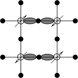
FIG. 1.: Cu-O planes and hyperfine couplings. The black dots mark the positions of the oxygen atoms, and the empty circles are the copper atoms with the electronic spins. The shaded areas symbolize the hyperfine coupling between a given oxygen site and the two neighboring copper spins.

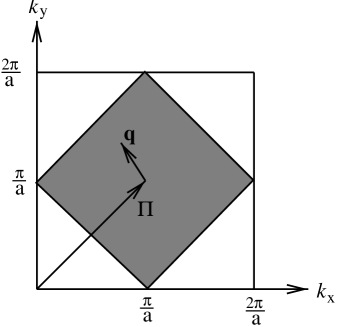
FIG. 2.: First Brillouin zone of a square lattice and reduced Brillouin zone of the antiferromagnet (shaded area). In the reduced zone scheme all wave-vectors ${\bf{q}}$ are measured with respect to the antiferromagnetic ordering wave-vector ${\bf{\Pi}}=(\pi/a,\pi/a)$.

REFERENCES

- [1] K. R. Thurber, A. W. Hunt, T. Imai, F. C. Chou, and Y. S. Lee, MIT preprint (1996, revised version February 1997), unpublished.
- [2] D. Beeman and P. Pincus, Phys. Rev. 166, 359 (1968).
- [3] F. Mila and T. M. Rice, Physica C 157, 561 (1989).
- [4] F. Mila and T. M. Rice, Phys. Rev. B 40, 11382 (1989).
- [5] S. Chakravarty and R. Orbach, Phys. Rev. Lett. 64, 224 (1990).
- [6] S. Chakravarty, P. M. Gelfand, P. Kopietz, R. Orbach, and M. Wollensak, Phys. Rev. B 43, 2796 (1991).
- [7] The form factor given in Eq.(A3) of Ref.[6] is too small by a factor of two; similarly, in Eq.(A4) of Ref.[6] a factor of four is missing.
- [8] P. C. Hohenberg, Phys. Rev. 158, 383 (1967); N. D. Mermin and H. Wagner, Phys. Rev. Lett. 17, 1133 (1966).
- [9] S. Chakravarty, in High Temperature Superconductivity: Proceedings, edited by K. S. Bedell et al. (Addison-Wesley, Redwood City, CA, 1990).
- [10] F. David, Nucl. Phys. B 190, [FS3], 205 (1981), and Comm. Math. Phys. 81, 149 (1981). See also G. Parisi, Statistical Field Theory, (Addison-Wesley, Redwood City, CA, 1988), page 197.
- [11] F. J. Dyson, Phys. Rev. 102, 1217 and 1230 (1956); S. V. Maleev, Zh. Eksp. Teor. Fiz. 30, 1010 (1957) [Sov. Phys.–JETP 6, 776 (1958)].
- [12] T. Holstein and H. Primakoff, Phys. Rev. 58, 1098 (1940).
- [13] A. B. Harris, D. Kumar, B. I. Halperin, and P. C. Hohenberg, Phys. Rev. B 3, 961 (1971).
- [14] As pointed out in P. Kopietz, Phys. Rev. B 48, 13789 (1993), in a sublattice formalism one should distinguish between two types of lattice--functions, namely and , where are the vectors of the reciprocal lattice associated with a sublattice, and is the usual Kronecker-. The function associates an extra minus sign with Umklapp scattering between two neighboring Brillouin zones. However, it turns out that in our calculation of all momentum sums are effectively cut off at , so that Umklapp scattering is not important. Therefore we may treat the function in Eq.(16) as a Kronecker delta .
- [15] P. W. Anderson, Phys. Rev. 86, 694 (1952).
- [16] P. Kopietz, Phys. Rev. B 41, 9228 (1990).
-
[17]
P. Kopietz, PhD thesis, University of California at Los Angeles, 1990 (unpublished).
The two-loop correction to the (staggered) dynamic structure factor
involves Feynman diagrams, while
another 16 diagrams should be considered for the
calculation of the second-order magnon damping.
Totally, it is thus necessary to consider
Feynman diagrams for obtaining the
numerical coefficient in Eq.(50).
Of course, some of these diagrams yield a vanishing contribution, but a priori
this is not obvious.
In order to keep this paper at a reasonable length and not to
overburden the reader with technical
details, we refrain from
listing these diagrams in the present work.
For interested readers we have
published the diagrams in the world wide web, see
http://www.theorie.physik.uni-goettingen.de/~kopietz/
- [18] The prefactor in Eq.(30) is twice as large as the prefactor given in Ref.[6]. This is due to the fact that the form factor used in Ref.[6] was too small by a factor of two.
- [19] T. Imai, private communication.
- [20] S. Chakravarty, B. I. Halperin, and D. R. Nelson, Phys. Rev. Lett. 60, 1057 (1988); Phys. Rev. B 39, 7443 (1989).