ITP-UH-2/97 January 1997

Properties of the chiral spin liquid state
in generalized spin ladders

Holger Frahm and Claus Rödenbeck

Institut für Theoretische Physik, Universität Hannover
D-30167 Hannover, Germany

We study zero temperature properties of a system of two coupled quantum spin chains subject to fields explicitly breaking time reversal symmetry and parity. Suitable choice of the strength of these fields gives a model soluble by Bethe Ansatz methods which allows to determine the complete magnetic phase diagram of the system and the asymptotics of correlation functions from the finite size spectrum. The chiral properties of the system for both the integrable and the nonintegrable case are studied using numerical techniques.

PACS-Nos.: 75.10.Jm, 75.30.Kz, 75.50.Ee

1 Introduction

The idea of a chiral spin liquid state spontaneously breaking parity ($P$) and time reversal ($T$) invariance has attracted considerable interest recently. It has first been proposed as a possible ground state for the two dimensional $S={1\over 2}$ Heisenberg model on a square lattice frustrated with a sufficiently strong antiferromagnetic next-nearest neighbour interaction [1]. Subsequent studies of this model have found an enhancement of a chiral order parameter, comparison with other possible states however suggests that the chiral spin state is unstable [2]. Different lattices, in particular the triangular and Kagomé one, have also been studied, however no firm evidence of a chiral spin state has been found so far. Here the frustration is a consequence of the lattice geometry.

To characterize a chiral phase several ‘order parameters’ have been introduced: For lattices built from triangular plaquettes the vector chirality [3]

$$\mathbf{X}={\mathbf{S}}_{1}\times{\mathbf{S}}_{2}+{\mathbf{S}}_{2}\times{\mathbf{S}}_{3}+{\mathbf{S}}_{3}\times{\mathbf{S}}_{1}$$ (1.1)

with ${\mathbf{S}}_{i}$ being the three spins on the corners of a triangular cell has been discussed. While a spontaneous symmetry breaking in $\mathbf{X}$ appears to be unlikely in an isotropic Heisenberg system its properties have been studied in stacked triangular antiferromagnets with XXZ type anisotropy [4, 5] which are realized in the ABX₃-type compounds such as CsCuCl₃ (see articles in [6]).

A rotationally invariant operator which has a non zero expectation value in a phase with broken $P$ and $T$ symmetry is defined through [1]

$$\widehat{\chi}_{{}_{\langle 123\rangle}}={\mathbf{S}}_{1}\cdot({\mathbf{S}}_{2}\times{\mathbf{S}}_{3})\ .$$ (1.2)

Finally, a topological “Cherns” number measuring the dependence of a quantum state on a twist in the boundary conditions has recently been introduced by Haldane and Arovas and used to characterize the ground state of a Heisenberg model on a hexagonal lattice subject to $PT$ breaking fields [7]. The actual computation of the Cherns number, however, is restricted to rather small systems thus limiting its use in studies of a phase diagram at present.

While the existence of a phase with spontaneous broken chirality in a frustrated two-dimensional Heisenberg model has not been established so far (a possible candidate may be the Kagomé lattice [8]) the experimental studies of ABX₃ compounds indicate that the frustration leads to a rich phase diagram if a magnetic field is applied [4, 9, 10].

Lacking a model with spontaneous broken $PT$-symmetry it is useful to consider models containing terms breaking these symmetries explicitly. Studies of such systems allow to gain a better understanding of the properties of the chiral spin liquid state and means for its characterization. In this paper we analyze a system of two spin-${1\over 2}$ Heisenberg chains coupled by exchange terms on diagonal bonds as shown in Fig. 1 described by the Hamiltonian

$${\cal H}_{0}=\sum_{n=1}^{2N}\left\{J_{1}{\mathbf{S}}_{n}\cdot{\mathbf{S}}_{n+1}+J_{2}{\mathbf{S}}_{n}\cdot{\mathbf{S}}_{n+2}\right\}$$ (1.3)

with periodic boundary conditions ${\mathbf{S}}_{2N+k}={\mathbf{S}}_{k}$ and even and odd indices labeling spins on the two sub chains respectively. For $J_{2}=0$ this is just the Bethe Ansatz soluble Heisenberg chain [11]. As long $J_{2}\leq J_{2c}\approx 0.25J_{1}$ the model continues to have gapless excitations above a translationally invariant ground state just as the single chain. Increasing the frustrating next-nearest neighbour interaction beyond $J_{2c}$ the system has two degenerate dimerized ground states leading to the Majumdar–Ghosh model with a simple dimer configuration for its ground states at $J_{2}={1\over 2}J_{1}$ [12].

To force the system into a chiral spin state we add terms breaking $PT$-symmetry explicitly

$${\cal H}_{\chi}=\frac{1}{2}\sum_{n=1}^{N}\left\{\chi_{1}\ {\mathbf{S}}_{2n-1}\cdot({\mathbf{S}}_{2n}\times{\mathbf{S}}_{2n+1})-\chi_{2}\ {\mathbf{S}}_{2n}\cdot({\mathbf{S}}_{2n+1}\times{\mathbf{S}}_{2n+2})\right\}\ .$$ (1.4)

Such multispin exchange terms may in fact be relevant for the description of certain realizations of the two dimensional Heisenberg model such as ³He layers on a graphite substrate [13]. Note, that the invariance under translations by one lattice site ($n\to n+1$) is destroyed by these term unless $\chi_{1}=-\chi_{2}$. For the full Hamiltonian including the chiral terms one has additional integrable models: for a “staggered” chiral field $\chi_{1}=-\chi_{2}$ the operator ${\cal H}_{\chi}$ is one of the hierarchy of integrals of motion of the Heisenberg chain, thus commutes with ${\cal H}_{0}(J_{2}=0)$. The consequences of the competition between these operators have been studied in [14]. Choosing the parameters in

$${\cal H}={\cal H}_{0}+{\cal H}_{\chi}$$ (1.5)

as

$$J_{1}=2(1-\kappa)\ ,\quad J_{2}=\kappa\ ,\quad\chi_{1}=\chi_{2}=2\sqrt{\kappa(1-\kappa)}\$$ (1.6)

one obtains a family of integrable models of generalized spin ladders introduced recently [15, 16, 17]. Varying of the free parameter $\kappa$ from 0 to 1 the system evolves from a single Heisenberg chain to a pair of decoupled ones, changing the sign of $\kappa$ reverses the sign of the chiral field, but doesn’t affect most other properties of the system.

Here we investigate the properties of the ground state and excitations of this model. In the following section the ground state energy and spectrum of the low lying excitations of the integrable model (1.6) are computed exactly. As in the Heisenberg chain the excitations over the antiferromagnetic (singlet) ground state are found to be spinons coming in pairs. For the characterization of the chiral properties we note that due to its quasi one dimensional character it is not possible to define an analogue of the topological Cherns number for this system. In the following we choose the expectation value of a uniform extension of the chirality (1.2) as a measure of the chirality

$$\widehat{\chi}=\frac{1}{N}\sum_{n=1}^{N}\left\{{\mathbf{S}}_{2n-1}\cdot({\mathbf{S}}_{2n}\times{\mathbf{S}}_{2n+1})-{\mathbf{S}}_{2n}\cdot({\mathbf{S}}_{2n+1}\times{\mathbf{S}}_{2n+2})\right\}\ .$$ (1.7)

Unfortunately, expectation values of operators not commuting with the Hamiltonian such as $\widehat{\chi}$ are not easily accessible within the framework of the Bethe Ansatz. Our results regarding $\langle\widehat{\chi}\rangle$ are obtained from numerical diagonalization of finite clusters. In Section 3 we study the phase diagram of the integrable model subject to a uniform external magnetic field ${\mathbf{h}}\parallel\hat{z}$. A characterization of the phases based on counting the number of gapless excitations supported by the system is possible from the Bethe Ansatz analysis. We identify three different phases in the $\kappa$–$h$ plane: for sufficiently large $h>h_{c2}$ the system shows saturated ferromagnetism. For ${1\over 4}<\kappa<1$ a phase with low lying excitations at four different wave numbers $\pm k_{1,2}$ is found for magnetic fields $h_{c1}<h<h_{c2}$ (a similar phase diagram has recently been established [18] in an integrable chain of alternating spins ${1\over 2}$ and $1$ [19]). To characterize these phases we can compute the magnetization again from the Bethe Ansatz while we have to rely on numerical results from finite systems for the chirality. In the final section we summarize our findings and comment on the properties of systems where the parameters $\chi_{1,2}$ are tuned away from the integrable point.

2 Ground state and excitations of the integrable model

As mentioned above, choosing the exchange constants for the Hamiltonian (1.5) as in (1.6) gives a system which is integrable by Bethe Ansatz methods. Starting from the ferromagnetic state with all $2N$ spins pointing up one can reduce the solution of the Schrödinger equation in the sector with $M$ overturned spins to a system of algebraic equations

$$\left(\frac{\lambda_{j}+\frac{\tilde{\kappa}}{2}+\frac{i}{2}}{\lambda_{j}+\frac{\tilde{\kappa}}{2}-\frac{i}{2}}\right)^{N}\left(\frac{\lambda_{j}-\frac{\tilde{\kappa}}{2}+\frac{i}{2}}{\lambda_{j}-\frac{\tilde{\kappa}}{2}-\frac{i}{2}}\right)^{N}=\prod_{j\not=k}^{M}\frac{\lambda_{j}-\lambda_{k}+i}{\lambda_{j}-\lambda_{k}-i}\ ,\qquad\tilde{\kappa}=\sqrt{\frac{\kappa}{1-\kappa}}$$ (2.1)

for the $M$ complex rapidities $\lambda_{j}$. Each solution of these Bethe Ansatz equations (2.1) corresponds to an eigenstate of ${\cal H}$ with spin $S=N-M=S^{z}$. Up to an overall constant the corresponding eigenvalues are given by

$$E(\{\lambda_{j}\})=\sum_{j=1}^{M}\left(\tilde{\epsilon}_{0}(\lambda_{j}+\frac{\tilde{\kappa}}{2})+\tilde{\epsilon}_{0}(\lambda_{j}-\frac{\tilde{\kappa}}{2})\right)+Mh,\quad\tilde{\epsilon}_{0}(\lambda_{j})=-\frac{1}{2}\frac{1}{\lambda_{j}^{2}+\frac{1}{4}}\ .$$ (2.2)

Here we have used the fact, that we are constructing eigenstates for fixed $S^{z}$, to include the effect of an external magnetic field in the Hamiltonian ${\cal H}\to{\cal H}-hS^{z}$.

A generic solution $\{\lambda_{j}\}$ of (2.1) is organized groups of uniformly spaced complex rapidities, so called strings

$$\lambda_{j}^{(m)}=x+i\mu_{j}\ ,\quad\mu_{j}=-\frac{m+1}{2},-\frac{m+3}{2},\ldots,\frac{m-1}{2}.$$ (2.3)

In the thermodynamic limit the ground-state is made up of real $\lambda$’s only (1-strings). Their density $\rho(\lambda)$ is given in terms of a linear integral equation

$$\rho(\lambda)+\int_{-\Lambda}^{\Lambda}d\mu K(\lambda-\mu)\rho(\mu)=\frac{1}{2\pi}\left(\frac{1}{(\lambda+\frac{\tilde{\kappa}}{2})^{2}+\frac{1}{4}}+\frac{1}{(\lambda-\frac{\tilde{\kappa}}{2})^{2}+\frac{1}{4}}\right)\ .$$ (2.4)

The kernel of this integral equation is $K(\lambda)=\frac{1}{2\pi}\,\frac{2}{\lambda^{2}+1}$. The dependence on the magnetic field is incorporated in the value of the integration boundaries $\Lambda$ which are to be chosen such that the total density is $\int_{-\Lambda}^{\Lambda}d\lambda\rho(\lambda)=(M/N)$. For a vanishing external magnetic field $h=0$ the ground state can be shown to be a singlet ($M=N$) and the rapidities fill the entire real axis resulting in $\Lambda=\infty$ in (2.4). Hence $\rho$ can be computed by Fourier transform, resulting in

$$\rho(\lambda)=\tilde{\rho}(\lambda+\frac{\tilde{\kappa}}{2})+\tilde{\rho}(\lambda-\frac{\tilde{\kappa}}{2}),\quad\mbox{with}\ \tilde{\rho}(\lambda)=\frac{1}{2\cosh(\pi\lambda)}.$$ (2.5)

From (2.2) the ground state energy $E_{0}$ per spin is given by [17]

$$\frac{E_{0}}{2N} = \frac{1}{2}\int_{-\infty}^{\infty}d\lambda\rho(\lambda)\epsilon_{0}(\lambda)=\int_{-\infty}^{\infty}d\lambda(\tilde{\rho}(\lambda+\frac{\tilde{\kappa}}{2})\tilde{\epsilon}_{0}(\lambda)+(\tilde{\rho}(\lambda-\frac{\tilde{\kappa}}{2})\tilde{\epsilon}_{0}(\lambda))$$ (2.6)

$$= -\ln 2-\frac{1}{4}(\Psi(1-\frac{i}{2}\tilde{\kappa})-\Psi(\frac{1}{2}-\frac{i}{2}\tilde{\kappa})+\Psi(1+\frac{i}{2}\tilde{\kappa})-\Psi(\frac{1}{2}+\frac{i}{2}\tilde{\kappa})).$$

The term containing digamma–functions $\Psi(x)$ increases from $-\ln 2$ to 0 as $\kappa$ varies between 0 and 1.

Low lying excitations of the system are parametrized by holes in the distribution of real $\{\lambda_{j}\}$. The dispersion of these spinons is determined by the integral equation for the dressed energies:

$$\epsilon(\lambda)+\int_{\epsilon(\lambda)<0}d\mu K(\lambda-\mu)\epsilon(\mu)=h-\frac{1}{2}\left(\frac{1}{(\lambda+\frac{\tilde{\kappa}}{2})^{2}+\frac{1}{4}}+\frac{1}{(\lambda-\frac{\tilde{\kappa}}{2})^{2}+\frac{1}{4}}\right).$$ (2.7)

In this grand canonical approach the ground state is characterized as the one in with all states with negative dressed energy $\epsilon(\lambda)$ are filled. For vanishing or sufficiently small (see below) magnetic fields this condition is related to that used in (2.4) above through $\epsilon(\pm\Lambda)=0$. Again, we can solve (2.7) by Fourier transform for $h=0$, giving

$$\epsilon(\lambda)=\tilde{\epsilon}(\lambda+\frac{\tilde{\kappa}}{2})+\tilde{\epsilon}(\lambda-\frac{\tilde{\kappa}}{2})\ , \quad\tilde{\epsilon}(\lambda)=\frac{\pi}{2\cosh(\lambda)}$$

$$k(\lambda)=\tilde{k}(\lambda+\frac{\tilde{\kappa}}{2})+\tilde{k}(\lambda-\frac{\tilde{\kappa}}{2})\ , \quad\tilde{k}(\lambda)=\arctan(\lambda)-\frac{\pi}{2}\ .$$ (2.8)

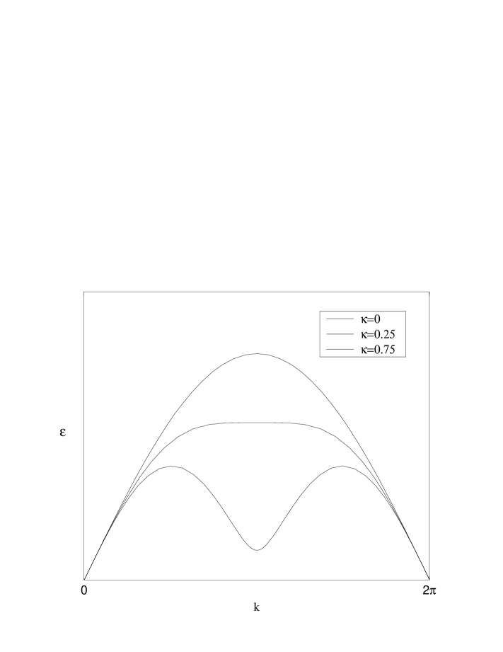
Figure 2: Spinon dispersion of the integrable model (1.6) for several values of $\kappa$.

Eliminating $\lambda$ from these equations one obtains the spinon dispersion $\epsilon(k)$ which is shown for several values of $\kappa$ in Figure 2.

Comparing these results with the known solution of the usual $S={1\over 2}$ XXX Heisenberg chain [20] we find that they coincide in the limits $\kappa\to 0,1$ as is expected from the Hamiltonian. Zero temperature quantities such as densities of rapidities or their dressed energies are simply superpositions of the corresponding quantities for the XXX chain with argument shifted by $\tilde{\kappa}$ (see (2.4), (2.7)). On the basis of the properties of the low lying excitations this comparison can be extended to the critical properties of the system: For zero $h$ the continuum limit of the system can be identified as a conformal field theory (CFT) with central charge $c=1$ for any $0\leq\kappa<1$. As for the XXX chain we expect this situation to be described by a level-1 SU(2) Wess-Zumino-Witten model. For $\kappa=1$ there appears another massless mode leading to low energy properties corresponding to two $c=1$ models (see also Section 3 below).

Finally we have studied the effect of the symmetry breaking terms ${\cal H}_{\chi}$ in the integrable Hamiltonian. It is instructive to start with the exact solution of a system of four spins (see also [1]). The Hamiltonian is given by (1.3) with $N=2$ and the couplings are

$$J_{1}=1,\quad J_{2},\quad\chi_{1}=\chi_{2}=:\kappa,\quad 0\leq\kappa\leq 1.$$ (2.9)

From the exact solution we know that the ground state of the integrable model is always a singlet. The same holds for the model given by (2.9). Hence it is sufficient to diagonalize the Hamiltonian in the two-dimensional singlet subspace. Depending on $J_{2}$ there are two distinct cases:

1. $J_{2}=\frac{1}{2}:\quad$ At the Majumdar–Ghosh point the singlets are degenerate for vanishing chiral field whereas for finite $\kappa$ the operator $\widehat{\chi}$ (1.7) lifts this degeneracy. One also observes that the Hamiltonian simplifies to ${\cal H}={\mathbf{S}}^{2}+\kappa\widehat{\chi}$ (up to a constant) and $[{\mathbf{S}}^{2},\widehat{\chi}]=0$. Therefore the chirality $\widehat{\chi}$ can be diagonalized in the singlet subspace, yielding a $\kappa$-independent chirality which is found to be one of its eigenvalues $\langle\widehat{\chi}\rangle=\pm\frac{1}{2}\sqrt{3}$.

2. $J_{2}\neq\frac{1}{2}:\quad$ Tuning $J_{2}$ away from $\frac{1}{2}$ the ground state of the $\kappa=0$-system is unique. At this point the Hamiltonian is $P$– and $T$–symmetric leading to a vanishing chirality in the ground state. Switching on the chiral field the two singlet eigenstates of the Hamiltonian have non-zero expectation values $\langle\widehat{\chi}\rangle$:

$$\langle\widehat{\chi}\rangle=\pm{{3}\over 2}\ {\kappa\over\sqrt{3\kappa^{2}+2(2J_{2}-{1})^{2}}}\ .$$ (2.10)

The “chiral susceptibility” $\partial\langle\widehat{\chi}\rangle/\partial\kappa$ diverges for $\kappa=0$ at the MG point. For $\kappa\gg 1$ the chirality approaches its eigenvalue $\frac{1}{2}\sqrt{3}$.

For larger systems no exact results on the chirality can be obtained (as mentioned in the introduction it is not possible to compute this expectation value directly from the Bethe Ansatz solution). For small systems (up to 24 spins) we have used a Lanzcos algorithm to compute some low lying states numerically. In Fig. 3 we present our results on ground state chirality from these data: $\langle\hat{\chi}\rangle$ vanishes for $\kappa\to 0,1$ as is expected from the single chain Hamiltonian in these limits. For intermediate values of $\kappa$ we find that the finite size corrections to the chirality are very small, so that the properties of the infinite system can easily be read off from the numerical data. We find that the maximum of the chirality is obtained at $\kappa\approx 0.58$ with about two thirds of the largest possible value $\sqrt{3}/2$.

3 Magnetic phase diagram of the integrable model

While the zero field properties of the model (1.5) are closely related to those of the single XXX Heisenberg chain, addition of an magnetic field gives rise to an interesting phase diagram (see Fig. 4): For small values of $\kappa$ we find that the magnetic field first breaks the SU(2) symmetry giving a $c=1$ Gaussian CFT with anomalous dimensions depending on the magnetic field. Increasing the magnetic field $h$ beyond a value $h_{c1}(\kappa)$ two additional “Fermi points” with gapless excitations arise, leading to a low energy spectrum as described by two $c=1$ Gaussian CFTs. Finally for magnetic field $h>h_{c2}$ the ground state of the system saturates ferromagnetically.

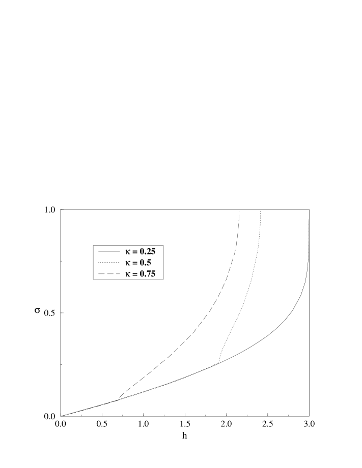
Figure 5: Magnetisation of the integrable model vs. magnetic field for three values of $\kappa$.

To calculate the corresponding phase boundaries as a function of $\kappa$ and the expectation values of the magnetization $\sigma=\langle S^{z}\rangle/(2N)$ as a function of the magnetic field we have to solve the integral equation (2.7). The numerical results for the magnetization are given in Figure 5.

Analytical results can be obtained near the critical field $h_{c2}$ which is determined from the condition that $\epsilon(\lambda)\geq 0$ for all values of $\lambda$. For fields $h\lessapprox h_{c2}$ the integral equation can be solved by iteration which allows to study the nature of low lying excitations and the dependence of the magnetization on $h$. Here one has to distinguish three different cases:

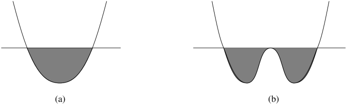
Figure 6: Filling fo the Fermi–Sea in presence of a magnetic field. Fig. (a): $\kappa<1/4$ and $0<h<h_{c2}$. Fig. (b): $\kappa>1/4$ and $h=h_{c1}$, the position of the ’kink’ in Figure 5.

(i) For $0\leq\kappa<{1\over 4}$ the minimum of the bare dispersion given by the driving terms in (2.7) is at $\lambda=0$ (see Fig. 6(a)). The dressed energies are nonnegative for magnetic fields

$$h\geq h_{c2}=4(1-\kappa)\ .$$ (3.1)

In this region the magnetization reaches its maximum according to a square root law

$$\sigma=1-\frac{2}{\pi}\sqrt{\frac{1}{h_{c2}-3}}\sqrt{h_{c2}-h}\ .$$ (3.2)

The system has massless excitations near the pseudo Fermi points $\epsilon(\pm\Lambda)=0$. Letting $h\to 0$ one finds that there is no additional phase transition, hence we can identify these excitations with the spinons forming the excitation spectrum at zero magnetic field. Standard techniques [21] can be used to compute the spectra of finite size systems from the Bethe Ansatz equations (2.1). The low lying energies compared to the ground state energy of the infinite system are ($L\equiv 2N$)

$$\Delta E=-{\pi\over 6L}v+{2\pi\over L}v\left(\Delta^{+}+\Delta^{-}\right)$$ (3.3)

where $v$ is the velocity of the massless magnons and the conformal dimensions of primary operators are

$$\Delta^{\pm}={1\over 2}\left\{{1\over 2\xi}\Delta M\pm\xi\Delta D\right\}^{2}\ .$$ (3.4)

$\Delta M$ is an integer denoting the change in $S^{z}$ induced by the operator, $\Delta D$ is an integer or half integer proportional to the momentum of the excited state (due to backscattering). The dressed charge $\xi=\xi(\Lambda)$ is given in terms of the linear integral equation $\xi(\lambda)+\int_{-\Lambda}^{\Lambda}d\mu K(\lambda-\mu)\xi(\mu)=1$. Depending on the external magnetic field it varies between $1/\sqrt{2}$ for $h=0$ and $1$ for $h\to h_{c2}$. The spectrum (3.3) allows to identify the central charge $c=1$ and the operator content of a Gaussian CFT with U(1) symmetry as mentioned above.

(ii) $\kappa={1\over 4}$: proceeding as in (i) one finds $h_{c2}=3$. Unlike for smaller $\kappa$ the dependence of the bare dispersion on the spectral parameter near the minimum is $\propto\lambda^{4}$. This leads to a different dependence of the magnetization on the field near $h_{c2}$:

$$\sigma=1-{4\over\pi}\left({3(h_{c2}-h)}\right)^{1\over 4}\ .$$ (3.5)

The classification of the low lying excitations as well as the interpretation concerning the conformal properties of the system coincide with those of case (i) above.

(iii) In the region ${1\over 4}<\kappa\leq 1$ two degenerate minima of the bare dispersion exist at nonzero values $\lambda=\pm\Lambda^{(0)}$ of the spectral parameter (Fig. 6(b)). This does not affect the dependence of the magnetization on the magnetic field for fields near the critical value

$$h_{c2}=1+\kappa^{-{1\over 2}}$$ (3.6)

As for $\kappa<{1\over 4}$ we have a square root dependence of $\sigma$ on $h\lessapprox h_{c2}$

$$\sigma=1-\hbox{const.}\ \sqrt{h_{c2}-h}$$ (3.7)

which a $\kappa$-dependent constant. The spectrum of low energy excitations, however, is different in this regime. For $h<h_{c2}$ there are two filled “Fermi seas” $[-\Lambda_{2},-\Lambda_{1}]$ and $[\Lambda_{1},\Lambda_{2}]$ of quasiparticles near $\pm\Lambda^{(0)}$ giving rise to two branches of massless spin excitations with different magnon velocities in the system. This situation is very similar to the one observed in the system with XY-type anisotropy and large staggered chiral field [14]: the expressions for the leading finite size corrections to the energies are (for the generalization of [21] to the case of several branches of excitations see also [22, 23])

$$\Delta E=-{\pi\over 6L}\left(v_{1}+v_{2}\right)+{2\pi\over L}\left(v_{1}(\Delta_{1}^{+}+\Delta_{1}^{-})+v_{2}(\Delta_{2}^{+}+\Delta_{2}^{-})\right)\ .$$ (3.8)

Here $v_{i}$ are the velocities of the excitations (linearized near the Fermi points $\pm\Lambda_{i}$) and the primary conformal dimensions $\Delta_{i}^{\pm}$ are found to be

$$\Delta_{i}^{\pm}={1\over 2}\left\{{{\xi_{i}^{+}\Delta M^{\pm}-\xi_{i}^{-}\Delta M^{\mp}}\over{2((\xi_{i}^{+})^{2}-(\xi_{i}^{-})^{2})}}\mp(\xi_{i}^{+}\Delta D^{\pm}+\xi_{i}^{-}\Delta D^{\mp})\right\}^{2}\ .$$ (3.9)

The numbers $\Delta M^{\pm}$ are the difference between the number of quasi particles in the Fermi seas in the ground state and excited state, respectively. $\Delta D^{\pm}$ counts the backscattering events in the excited state (giving rise to excitations with momenta being multiples of twice the Fermi momenta of the quasiparticles). All conformal dimensions can be parametrized by the four numbers $\xi_{i}^{\pm}=\xi^{\pm}(\Lambda_{i})$ which are given in terms of the integral equations

$$\xi^{+}(\lambda)=1-\int_{\Lambda_{1}}^{\Lambda_{2}}K(\lambda-\mu)\xi^{+}(\mu)-\int_{\Lambda_{1}}^{\Lambda_{2}}K(\lambda+\mu)\xi^{-}(\mu)\ ,$$

$$\xi^{-}(\lambda)=-\int_{\Lambda_{1}}^{\Lambda_{2}}K(\lambda+\mu)\xi^{+}(\mu)-\int_{\Lambda_{1}}^{\Lambda_{2}}K(\lambda-\mu)\xi^{-}(\mu)\ .$$ (3.10)

(3.8) is the generic form of a low energy spectrum in a system with two different branches of massless excitations. A finite size spectrum of the form (3.8) arises in many one dimensional systems, e.g. integrable spin chains [22, 24, 14] and various models of correlated electrons [23, 25] where the two critical degrees of freedom are holon and spinon excitations. In the present model it can be interpreted as a realization of two $c=1$ Gaussian models.

Decreasing the magnetic field further the universality class changes again at $h=h_{c1}$ where $\Lambda_{1}=0$ and $v_{1}$ vanishes leading to a divergence of the low temperature specific heat $C\approx(\pi T/6)\left(v_{1}^{-1}+v_{2}^{-1}\right)$. At this point one of the massless modes has a quadratic dispersion and the system undergoes a Pokrovsky–Talapov transition into the U(1) Gaussian phase with central charge $c=1$ that was already identified for $\kappa<{1\over 4}$ above. The value of $h_{c1}$ has to be determined by numerical solution of the integral equations (2.7). The complete magnetic phase diagram is shown in Fig. 4.

This phase transition leads to a discontinuous change in the spectrum of critical exponents determining the long distance asymptotics of the correlation functions of the system. As an example we consider the spin spin correlator $C^{zz}(x)=\langle S_{x}^{z}S_{0}^{z}\rangle$. The massless magnon excitations discussed above lead to algebraically decaying correlation functions, from (3.4) and (3.9) we find that the leading term in $C^{zz}$ beyond the constants is of the form $(1/x)^{\alpha}\ \cos(2k_{0}x)$ where $k_{0}$ is a magnetic field dependent wave number and the exponent $\alpha$ is given by

$$\alpha=\left\{\begin{array}[]{cl}2\xi^{2}&\mathrm{for~{}}0\leq h<h_{c1}\\ \sum_{i}\left((\xi^{+}_{i})^{2}+(\xi^{-}_{i})^{2}\right)&\mathrm{for~{}}h_{c1}<h<h_{c2}\\ \end{array}\right.\ .$$ (3.11)

For $h\to 0$ ($h_{c2}$) one obtains $\alpha=1$ ($2$) from the appropriate expression as in region (i). In Fig. 7 the values of the exponent $\alpha$ as $h_{c1}$ is approached from above and below are presented as a function of $\kappa$. For ${1\over 4}<\kappa<1$ one observes a discontinuous increase of $\alpha$ at the transition $h=h_{c1}$. Such a change of the asymptotic behaviour of $C^{zz}$ can be observed e.g. in the temperature dependence of NMR longitudinal relaxation rate, $1/T_{1}\propto T^{\alpha-1}$.

Finally we want to note that that these pronounced features in the $h$-dependence of the magnetization and the critical behaviour of the system are reflected in the chirality properties of the system: Numerical computation of the chirality in the ground state as a function of the applied magnetic field for systems with up to 24 spins shows a smooth dependence of $\langle\widehat{\chi}\rangle$ on the magnetization. At the same time the fluctuations $\langle\left(\Delta\widehat{\chi}\right)^{2}\rangle$ scale like $1/N$ for $h<h_{c1}$ and are enhanced as the critical field is approached from below. Above $h_{c1}$ they become smaller vanishing for the ferromagnetic state (see Figure 8).

4 Summary and conclusion

We have present results on the ground state properties and the magnetic phase diagram of a quasi one-dimensional spin-system with explicitly $P$ and $T$ breaking terms in the Hamiltonian. These terms generate chiral order in the system which in turn is found to lead to an interesting behaviour of the system when exposed to an external magnetic field.

The question remains to which extent the observed behaviour is determined by the integrability of the system (1.5), (1.6). While a complete analyisis of this question is difficult we have diagonalized small systems to give a partial answer:

Choosing the parameters as in (2.9) with $J_{2}={1\over 2}$ the system interpolates between two soluble points: For $\kappa=0$ the model reduces to the MG–model, $\kappa=\frac{1}{2}$ is the Bethe Ansatz soluble point. While the former one has a gap for spin excitations, the latter supports massless magnons. The vanishing of this spin gap as a function of $\kappa$ has been studied using Lanzcos procedures and finite size interpolation. At the MG–point the gap above the two degenerate valence bond singlets is known very accurately, being $\Delta_{MG}=0.236$ with finite size corrections scaling as $\Delta^{2}=\Delta_{MG}^{2}(1+\mathrm{const.}/{N^{2}})$ [26]. At $\kappa=\frac{1}{2}$ the gap vanishes as $\Delta\sim\mathrm{const}/{N}$ according to (3.4). It is difficult to find an interpolating expression between these limiting cases that leads to uniformly good fits of the numerical data. Still one can conclude that inclusion of the chiral term results in a rapidly vanishing gap, as can be seen in Figure 9. For $\kappa\gtrapprox 0.15$ the numerical data do not allow to decide whether there is a finite gap or not. The ground state expectation value of the chirality shows a monotonic increase with $\kappa$, with $\langle\widehat{\chi}\rangle\approx 0.58$ at $\kappa=1$.

Further studies are necessary for a better understanding of the intermediate phase transition in the integrable model at $h=h_{c1}$. At $h=0$ this transition occurs at the point $\kappa=1$, corresponding to a decoupling of the two sublattices. Whether such a ‘dimensional reduction’ is the origin of the phase transition at $\kappa<1$ and whether this feature can be used to describe the experimentally observed magnetic phases in the frustrated ABX₃ compounds remains to be investigated in the context of systems with a larger number of coupled chains and eventually truly two-dimensional lattices.

Figure 1: Lattice on which the spin Hamiltonian (1.3) is defined: The two-spin exchange coupling is $J_{1}$ and $J_{2}$ on full and dashed lines, respectively. The three spin exchange $\propto\chi_{1,2}$ couples the spins on the corners of each triangle.

Figure 3: Chirality of the integrable Model (1.6). The system sizes are $2N=8,12,16,20,24,\infty$ from top to bottom.

Figure 4: Magnetic phase diagram of the integrable system. Below $h_{c1}$ the system has central charge $c=1$, for $h_{c1}<h<h_{c2}$ the model is a realization of two $c=1$ models, and for $h>h_{c2}$ the system saturates in a fully polarized (ferromagnetic) state.

Figure 7: Critical exponent $\alpha$ of $\langle S^{z}_{x}S^{z}_{0}\rangle$ as a function of $\kappa$ for magnetic field $h\to h_{c1}$ from below (dashed line) and above (full line).

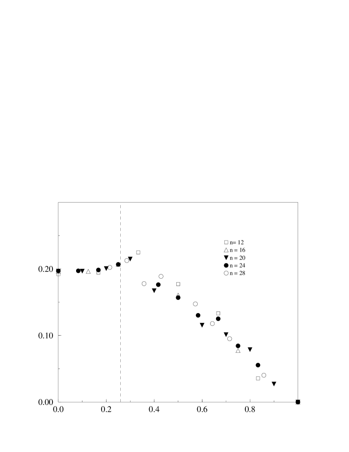
Figure 8: Chiral fluctuations $\langle\left(\Delta\widehat{\chi}\right)^{2}\rangle$ in the ground state for given magnetization $\sigma$ of the integrable system with $\kappa={1\over 2}$ and $n$ spins. The dashed line indicates the value of the magnetization at the critical magnetic field $h_{c1}$ for the infinite system.

Figure 9: Spin gap $\Delta$ for $J_{1}=2J_{2}=1$ as a function of the strength of the chiral field. The line is guide for the eyes and is given by a Gaussian.

References

- [1] X. G. Wen, F. Wilczek, and A. Zee, Phys. Rev. B 39, 11413 (1989).
- [2] M. Imada, J. Phys. Soc. Japan 58, 2650 (1989); H. Shiba and M. Ogata, J. Phys. Soc. Japan 59, 2971 (1990); D. Poilblanc, E. Gagliano, S. Bacci, and E. Dagotto, Phys. Rev. B 43, 10970 (1991).
- [3] S. Miyashita and H. Shiba, J. Phys. Soc. Japan 53, 1145 (1984); S. Fujiki and D. D. Betts, Can. J. Phys. 65, 76 (1987).
- [4] T. Nikuni and H. Shiba, J. Phys. Soc. Japan 62, 3268 (1993).
- [5] S. V. Maleyev, Phys. Rev. Lett. 75, 4682 (1995).
- [6] Magnetic systems with competing interactions (Frustrated spin systems), edited by H. T. Diep (World Scientific, Singapore, 1994).
- [7] F. D. M. Haldane and D. P. Arovas, Phys. Rev. B 52, 4223 (1995).
- [8] C. Lhuillier, private communication.
- [9] M. Mino, K. Ubukata, T. Bokui, M. Arai, H. Tanaka, and M. Motokawa, Physica B 201, 213 (1994).
- [10] N. Stüßer, U. Schotte, K. D. Schotte, and X. Hu, Physica B 213, 164 (1995).
- [11] H. Bethe, Z. Phys. 71, 205 (1931).
- [12] C. K. Majumdar and D. K. Ghosh, J. Math. Phys. 10, 1388 (1969); ibid. 1399 (1969).
- [13] H. Godfrin, R. R. Ruel, and D. D. Osheroff, Phys. Rev. Lett. 60, 305 (1988).
- [14] H. Frahm, J. Phys. A 25, 1417 (1992).
- [15] V. Yu. Popkov and A. A. Zvyagin, Phys. Lett. A 175, 295 (1993).
- [16] C. Rödenbeck, Diploma thesis, Universität Hannover, 1994.
- [17] H. Frahm and C. Rödenbeck, Europhys. Lett. 33, 47 (1996).
- [18] M. Fujii, S. Fujimoto, and N. Kawakami, J. Phys. Soc. Japan 65, 2381 (1996).
- [19] H. J. de Vega and F. Woynarovich, J. Phys. A 25, 4499 (1992); B.-D. Dörfel and S. Meißner, J. Phys. A 29, 6471 (1996).
- [20] L. D. Faddeev and L. A. Takhtajan, J. Sov. Math. 24, 241 (1984), [Zap. Nauch. Semin. LOMI 109, 134 (1981)].
- [21] H. J. de Vega and F. Woynarowich, Nucl. Phys. B 251, 439 (1985).
- [22] A. G. Izergin, V. E. Korepin, and N. Yu. Reshetikhin, J. Phys. A 22, 2615 (1989).
- [23] F. Woynarovich, J. Phys. A 22, 4243 (1989).
- [24] H. Frahm and N.-C. Yu, J. Phys. A 23, 2115 (1990).
- [25] H. Frahm and V. E. Korepin, Phys. Rev. B 42, 10533 (1990); ibid. B 43, 5653 (1991); N. Kawakami and S.-K. Yang, J. Phys. Condens. Matter 3, 5983 (1991).
- [26] T. Tonegawa and I. Harada, J. Phys. Soc. Japan 56, 2153 (1987); K. Sano and K. Takano, J. Phys. Soc. Japan 62, 2809 (1993).