[

Correlation Lengths in Quantum Spin Ladders

Abstract

Analytic expressions for the correlation length temperature dependences are given for antiferromagnetic spin–1/2 Heisenberg ladders using a finite–size non–linear $\sigma$–model approach. These calculations rely on identifying three successive crossover regimes as a function of temperature. In each of these regimes, precise and controlled approximations are formulated. The analytical results are found to be in excellent agreement with Monte Carlo simulations for the Heisenberg Hamiltonian.

]

Low–dimensional quantum magnets exhibit many novel collective low–temperature properties. An interesting recent development is the system of spin ladders [1] that are arrays of $n$ coupled antiferromagnetic Heisenberg chains. Experiments and numerical studies have revealed many fascinating aspects of these systems, such as the surprise that spin–1/2 ladders composed of an even number of chains have a gap in the excitation spectrum, while those with an odd number of chains are gapless [2].

For the two–dimensional square–lattice spin–1/2 Heisenberg antiferromagnet with nearest–neighbor interactions, theoretical predictions for the spin–spin correlation length based on the (2+1)–dimensional non–linear $\sigma$–model [3] are in excellent quantitative agreement with neutron scattering results [4]. In Ref. [5], one of us pointed out that it is useful to view a spin ladder as a finite–sized two–dimensional antiferromagnet, instead of a system of coupled spin chains. The zero–temperature properties could then be readily obtained from the finite–size scaling of the (2+1)–dimensional non–linear $\sigma$–model, where one of the spatial directions is finite and the remaining directions infinite, one of them being the Euclidean time direction. In this manner one could obtain both a clear picture of the dimensional crossover to the two–dimensional square–lattice antiferromagnet, as well as precise analytical estimates of the zero–temperature correlation lengths and gaps in spin ladders. Moreover, it was predicted that the spin gap, $\Delta$, is simply related to the spin–spin correlation length, $\xi$, such that

$$\left(\frac{\Delta}{J}\right)\left(\frac{\xi}{a}\right)=\left(\frac{\hbar c}{Ja}\right),$$ (1)

where $J$ is the antiferromagnetic coupling, $a$ is the lattice spacing, and $c$ is the physical spin wave velocity of the two–dimensional square lattice antiferromagnet at zero temperature. Applied to $S=1/2$, the right hand side of Eq. (1) should be 1.68.

At first sight, an analysis at non–zero temperatures similar to that at zero temperature may appear formidable. One of the purposes of this paper is to show that this is not so. Once one recognizes three distinct crossover scales as a function of temperature, the temperature dependence of the correlation length can be computed with equal ease. In the language of the $\sigma$–model, the system is a box whose two sides $L_{y}=na$ (the spatial direction along the width of the ladders) and $\beta\hbar c$ (the Euclidean time direction) are finite in extent, where $\beta$ is the inverse temperature. Successive crossovers take place as the system goes through regimes where $\beta\hbar c\gg L_{y}$, $\beta\hbar c\sim L_{y}$, and $\beta\hbar c\ll L_{y}$. (There is an additional crossover at even higher temperatures, where the system becomes entirely classical, which is not discussed here.) In each of these three regimes, it is possible to formulate precise and controlled analytical methods to compute correlation lengths of spin ladders. These estimates are then tested against new numerical simulations, and we find excellent agreement between the numerical and the analytical results. Because we use periodic boundary conditions across the width of the ladders in the $\sigma$–model approach [6], it is necessary for us to carry out simulations with periodic boundary conditions as well. However, we show that the choice of boundary conditions hardly matters for ladders of width larger than $n=4$. Finally, we show that the zero–temperature predictions of the correlation lengths [5, 7], that contain no adjustable parameters, are in good agreement with the simulation results, and that the relation shown in Eq. (1) holds with remarkable accuracy. Thus, we believe that we have a reasonably complete picture of spin fluctuations in spin ladders.

The Hamiltonian for a Heisenberg ladder is

$$H=J_{\|}\sum_{\langle ij\rangle_{\|}}{\bf S}_{i}\cdot{\bf S}_{j}+J_{\bot}\sum_{\langle ij\rangle_{\bot}}{\bf S}_{i}\cdot{\bf S}_{j},$$ (2)

where ${\bf S}_{i}=\frac{1}{2}{\bf\sigma}_{i}$ is the quantum spin operator at site $i$, while $\langle ij\rangle_{\|}$ and $\langle ij\rangle_{\bot}$ denote nearest neighbors along and between chains, respectively. The couplings considered are isotropic and antiferromagnetic, that is, $J_{\|}=J_{\bot}=J$ and $J>0$. As in the previous study [8], the ladders are investigated with a very efficient loop cluster algorithm [9]. The correlation length is obtained from the exponential large–distance decay of the measured instantaneous spin–spin correlation function. We refine the original simulations with open boundary conditions [8], and repeat them with periodic boundary conditions. These calculations yield low–T correlation lengths, $\xi/a$, of 7.1(1) and 10.3(1) for ladders of width $n=4$ for periodic and open boundary conditions, respectively. The results for $n=6$ are 30.5(10) and 32.0(10) for periodic and open boundary conditions, respectively. Our corresponding analytical results for the periodic boundary condition are 6.2 and 26.2 for $n=4$ and $n=6$, respectively[5, 7]. The spin gaps are obtained from independent numerical measurements of the uniform susceptibility. For $n=4$ they are 0.234(4) and 0.160(4) for periodic and open boundary conditions, respectively. Similarly, for $n=6$, we obtain 0.055(4) and 0.053(4), respectively, for periodic and open boundary conditions. It is seen that Eq. (1) holds remarkably well. The temperature dependence of the correlation lengths obtained from Monte Carlo simulations are shown in Fig. (1). For $n=6$, the choice of boundary conditions indeed hardly matters.

FIG. 1.: Correlation lengths obtained from Monte Carlo simulations as functions of temperature for spin–1/2 ladders composed of four and six chains.

By studying the effective Euclidean action of the (2+1)–dimensional non–linear $\sigma$–model,

$$\frac{S}{\hbar}=\frac{\rho_{s}^{0}}{2\hbar}\int_{0}^{\beta\hbar}d\tau\int dx\int_{0}^{L_{y}}dy\left[\left(c^{-1}\partial_{\tau}\hat{\Omega}\right)^{2}+\left(\partial_{\mu}\hat{\Omega}\right)^{2}\right],$$ (3)

where $\mu$ is to be summed over the spatial directions, $x$ and $y$, we calculate the temperature dependence of the correlation length in three distinct regimes characterized by the ratio $\beta\hbar c/L_{y}$. The parameter $\rho_{s}^{0}$ is the bare spin stiffness constant at the spatial cutoff $\Lambda^{-1}$ of the model, $c$ is the spin–wave velocity defined on the same scale and $\hat{\Omega}$, the staggered order parameter field, is a three-component unit vector. In the low–T ($\beta\hbar c\gg L_{y}$) and high–T ($\beta\hbar c\ll L_{y}$) regimes we map (3) to a (1+1)–dimensional quantum nonlinear $\sigma$–model where the spatial dimension refers to the $x$–direction, and the extent of the “time–direction” is $\beta\hbar c$ and $L_{y}$, respectively. For the intermediate–T ($\beta\hbar c\sim L_{y}$) regime the effective model is the one–dimensional classical non–linear $\sigma$–model. The fluctuations that are integrated out are approximated by a one–loop modification of the coupling constant for the effective theory.

FIG. 2.: The three different temperature regimes: a) low–T, b) intermediate–T, and c) high–T. The figures show the extensions of the two finite directions. For a) and c), the effective model is a (1+1)–dimensional quantum non–linear $\sigma$–model with fields constant in the shortest directions, and a coupling modified by the fluctuations in this direction. For b), the fields are constant along both the $y$– and $\tau$–directions, and the effective model is a one–dimensional classical $\sigma$-model.

Figure (2) illustrates the situations in the three different regimes.

At $T=0$ the “Lorentz”–invariance of the non–linear $\sigma$–model gives the simple relation Eq. (1) between the correlation length and the gap. For $T\neq 0$ it is not so clear that the spin–wave velocity will survive quantum fluctuations unrenormalized. However, it is certainly the case that the quantum fluctuations at the one–loop level cannot renormalize the spin–wave velocity at any temperature. Therefore, within our one–loop approximation, it is consistent to promote Eq. (1) to be valid at all temperatures, which we will do.

For low temperatures, the same procedure as that used for the $T=0$ calculation[5], of integrating out the fluctuations along the finite–width ($y$–direction) to one–loop order, should work. However, at non–zero temperatures the resulting effective model is not the two–dimensional classical non–linear $\sigma$–model, but a (1+1)–dimensional quantum non–linear $\sigma$–model,

$$\frac{S}{\hbar}=\frac{1}{2\epsilon(L_{y},T)}\int dx\int_{0}^{\beta\hbar c}du\left[\left(\partial_{u}\hat{\Omega}\right)^{2}+\left(\partial_{x}\hat{\Omega}\right)^{2}\right],$$ (4)

where

$$\frac{1}{\epsilon(L_{y},T)} = \frac{1}{\epsilon(L_{y},0)}$$ (5)

$$- \int\frac{dk}{2\pi}\sum_{m=-\infty}^{\infty\;\;\prime}\frac{\left[k^{2}+k_{m}^{2}\right]^{-1/2}}{\exp{\left[\beta\hbar c\Lambda\sqrt{k^{2}+k_{m}^{2}}\right]}-1}.$$ (6)

The effects of the fluctuations in the $y$–direction are taken into account by modifying the coupling constant to one–loop order; for convenience, we separate out the temperature–independent part, $\epsilon(L,0)$. In the above expression $k_{m}=2\pi m/L\Lambda$, and the prime on the summation sign means that the $m=0$ term is omitted from the sum. This expression is valid for ladders with periodic boundary conditions in all directions. In this Letter we only consider spin ladders with these boundary conditions. A short wavelength cutoff is imposed on the integration and on the summation such that $\sqrt{k^{2}+k_{m}^{2}}<1$, where $\Lambda$ is the cutoff scale chosen to conserve the area of the first Brillouin zone: $\Lambda a=2\sqrt{\pi}$. The results are only weakly dependent on this choice. Because of the absence of the topological term, the above action only describes spin–1/2 ladders of even width.

The correlation length for the above model (4) can be obtained from a simple self–consistent approach. By relaxing the unitarity condition on $\hat{\Omega}$ and adding a mass term, the condition $<\Omega^{2}>=1$ yields

$$N\epsilon(L_{y},T)\int_{0}^{1}\frac{dk}{2\pi}\frac{\coth{\left(\sqrt{k^{2}+\tilde{\Delta}^{2}(L_{y},T)}\beta\hbar c\Lambda/2\right)}}{\sqrt{k^{2}+\tilde{\Delta}^{2}(L_{y},T)}}=1,$$ (7)

where $N=3$ and $\tilde{\Delta}=(\Lambda\xi)^{-1}$. Solving this equation at $T=0$ gives

$$\tilde{\Delta}(L,0)=\frac{1}{\sinh{\left(2\pi/N\epsilon(L_{y},0)\right)}}.$$ (8)

Unfortunately this is not the correct zero–temperature result[5, 7]. To remedy this we can let $N\epsilon(L_{y},0)$ be a free parameter and adjust it such that $\Delta(L_{y},0)$ agrees with the correct zero–T result[5]. Fixing $N\epsilon(L_{y},0)$ in this way we can solve Eq. (6) numerically for the correlation length at non–zero temperatures. Due to the slight discrepancy between the $T=0$ correlation lengths given in [5] and the correlation lengths obtained in the Monte Carlo simulations we adjust $N\epsilon(L_{y},0)$ such that the $T=0$ correlation length agrees with the Monte Carlo data, that is $\xi/a$=7.1 and 30.5 for $n=4$ and $n=6$, respectively. The finite–T correlation lengths for these ladders are shown in region I in Fig. (3).

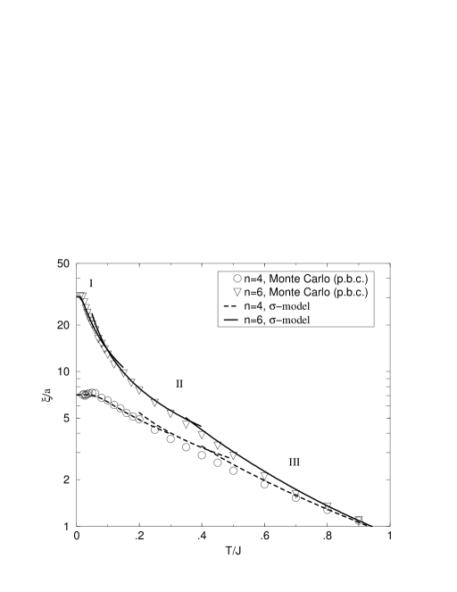
FIG. 3.: Correlation lengths as functions of temperature in the three distinct regimes for spin ladders of width $n=4$ and $n=6$, compared with the data from numerical simulations. The three regimes are labeled: I) low–T, II) intermediate–T, and III) high–T.

For intermediate temperatures, $\beta\hbar c\sim L_{y}$, the fluctuations in both the $y$– and the $\tau$–directions are integrated out. The low–energy effective action is then a one–dimensional classical non–linear $\sigma$–model,

$$\frac{S}{\hbar}=\frac{1}{2t(L_{y},T)}\int dx\left(\partial_{x}\hat{\Omega}\right)^{2},$$ (9)

where the coupling constant to one–loop order is

$$t^{-1}(L_{y},T)=\beta L\rho_{s}^{0}-\int\frac{dq}{2\pi}\sum_{m,n}^{\;\;\prime}\frac{1}{q^{2}+q_{m}^{2}+\omega_{n}^{2}}.$$ (10)

Here, $q_{m}=2\pi m/L_{y}$, $\omega_{n}=2\pi n/\beta\hbar c$, and the prime on the sum indicates that the $m=n=0$ term is omitted. Using a combination of Ewald and Poisson summation techniques, as in Ref. [10], we get

$$t^{-1}(L_{y},T)=\frac{L_{y}\beta\hbar c}{\xi_{J}}+L_{y}A(\frac{\beta\hbar c}{L_{y}}),$$ (11)

where $\xi_{J}$ is the Josephson length in the Néel phase[5], and the scaling function $A$ is

$$A(x)=\frac{\sqrt{x}}{2\pi}\left[\int_{1}^{\infty}dyy^{-1/2}\left(X(\pi xy)X(\pi y/x)-1\right)-2\right],$$ (12)

where

$$X(y)=\sum_{n=-\infty}^{\infty}e^{-yn^{2}}.$$ (13)

The one–dimensional classical $\sigma$–model is nothing but the continuum limit of the classical Heisenberg spin chain on a lattice, which has the action

$$S=-K\sum_{i}\hat{\Omega}_{i}\cdot\hat{\Omega}_{i+1}.$$ (14)

The correlation length for this lattice model has been calculated exactly in [11], and is

$$\frac{\xi}{a}=-\frac{1}{\ln\left[\coth K-1/K\right]}.$$ (15)

Taking the continuum limit $a\to 0$, with $Ka$ kept fixed, we find

$$S=\frac{Ka}{2}\int dx\left(\partial_{x}\hat{\Omega}\right)^{2}+const.$$ (16)

The one–dimensional non–linear $\sigma$–model is a finite theory for which no ultraviolet regularization is necessary, and there are no ambiguities associated with taking the continuum limit. Thus from Eqs. (9) and (16) we can identify $Ka=1/t(L_{y},T)$. Taking the continuum limit of Eq. (15), with $Ka$ held fixed, we obtain

$$\frac{\xi}{a}=\frac{t^{-1}(L_{y},T)}{a}.$$ (17)

We note that this expression has no adjustable parameters. The results for ladders composed of four and six chains are shown in region II of Fig. (3).

For temperatures such that $L_{y}\gg\beta\hbar c$, it is reasonable to map the action Eq. (3) to a (1+1)–dimensional quantum non–linear $\sigma$–model in which the “time direction” is really the width $L_{y}=na$ of the ladders,

$$\frac{S}{\hbar}=\frac{1}{2f(L_{y},T)}\int dx\int_{0}^{L_{y}}dy\left[\left(\partial_{x}\hat{\Omega}\right)^{2}+\left(\partial_{y}\hat{\Omega}\right)^{2}\right].$$ (18)

Here, the effective coupling constant is

$$\frac{1}{f(L_{y},T)} = \frac{1}{f(\infty,T)}$$ (19)

$$- \int\frac{dk}{2\pi}\sum_{n=-\infty}^{\infty\;\;\prime}\frac{\left[k^{2}+\omega_{n}^{2}\right]^{-1/2}}{\exp{\left[L_{y}\Lambda\sqrt{k^{2}+\omega_{n}^{2}}\right]}-1},$$ (20)

and $\omega_{n}=2\pi n/\beta\hbar c\Lambda$. This is very similar to the low–T case; one just has to interchange $\beta\hbar c$ with $L_{y}$. In the low–temperature regime, we imposed a cutoff in the two spatial directions. Here, it is convenient to impose the cutoff in the $x-\tau$–plane. We have checked that this change in the cutoff procedure does not alter the results. In the same way as for the low–temperature regime we find the correlation length by a self–consistent equation,

$$Nf(L_{y},T)\int_{0}^{1}\frac{dk}{2\pi}\frac{\coth{\left(\sqrt{k^{2}+\tilde{\Delta}^{2}(L_{y},T)}L_{y}\Lambda/2\right)}}{\sqrt{k^{2}+\tilde{\Delta}^{2}(L_{y},T)}}=1.$$ (21)

The quantity $Nf(\infty,T)$ is adjusted such that the solution of the equation at $L_{y}=\infty$, $\xi(\infty,T)$, corresponds to the correlation length of the (2+1)–dimensional quantum antiferromagnet which was calculated in [3, 13],

$$\frac{\xi(\infty,T)}{a}=\frac{e\sqrt{2}Z_{c}}{8\pi SZ_{\rho_{s}}}e^{2\pi S^{2}Z_{\rho_{s}}J/T}\left(1-\frac{1}{4\pi S^{2}Z_{\rho_{s}}}\frac{T}{J}\right),$$ (22)

where $Z_{c}=1.19$ and $Z_{\rho_{s}}=0.740$[14]. Having fixed $Nf(\infty,T)$, we calculate $\xi(L_{y},T)$ by solving (21) numerically. The results for $n=4$ and $n=6$ correspond to region III of Fig. (3).

It is evident from Fig. (3) that the analytic results for the correlation lengths agree remarkably well with the numerical simulations on even–legged spin–1/2 ladders with periodic boundary conditions. Since our effective non–linear $\sigma$–model does not contain the topological term, our results are strictly valid for even–leg ladders. However, the topological term is important only for the physics[5] at very low energies. Thus, we expect that our expressions for the intermediate– and high–temperature regimes are valid also for odd–leg ladders. It would, however, be interesting to have a more quantitative understanding of the crossover to the WZW–model for odd–legged spin ladders.

O.F.S. and S.C. were supported by a grant from the National Science Foundation, Grant No. DMR-9531575. M.G. would like to thank R. J. Birgeneau and U.–J. Wiese for many stimulating discussions, and was supported by the MRSEC Program of the NSF under Award No. DMR 94-00334 and by the International Joint Research Program of NEDO (New Energy Industrial Technology Development Organization, Japan).

REFERENCES

- [1] D. C. Johnston et al., Phys. Rev. B 35, 219 (1987); Z. Hiroi et al., J. Solid State Chen. 95, 230 (1991); M. Azuma et al., Phys. Rev. Lett. 73, 3463 (1994); K. Kojima et al., Phys. Rev. Lett. 74, 2812 (1995).
- [2] For a review, see E. Dagotto and T. M. Rice, Science 271, 618 (1996) and references therein.
- [3] S. Chakaravarty, B. I. Halperin, and D. R. Nelson, Phys. Rev. B 39, 2344 (1989).
- [4] M. Greven et al., Z. Phys. B 96, 465 (1995).
- [5] S. Chakravarty, Phys. Rev. Lett. 77, 4450 (1996).
- [6] M. A. Martin-Delgado and G. Sierra (private communications) have investigated the case of Dirichlet boundary condition.
- [7] See also, G. Sierra, preprint, cond-mat/9610057.
- [8] M. Greven, R. J. Birgeneau, and U. -J. Wiese, Phys. Rev. Lett. 77, 1865 (1996).
- [9] H. G. Evertz, G. Lana, and M. Marcu, Phys. Rev. Lett. 70, 875 (1993); U.–J. Wiese and H.–P. Ying, Z. Phys. B 93, 147 (1994).
- [10] J. Rudnick, H. Guo, and D. Jasnow, J. Stat. Phys. 41, 353 (1985).
- [11] M. E. Fisher, Amer. Jour. Phys. 32, 343 (1964).
- [12] D. Khveshchenko, Phys. Rev. B 50, 380 (1994); G. Sierra, J. Phys. A 29, 3299 (1996).
- [13] We use the prefactor of P. Hasenfratz and F. Niedermayer, Phys. Lett. B 268, 231 (1991).
- [14] R. R. P. Singh, Phys. Rev. B 39, 9760 (1989); R. R. P. Singh and D. Huse, Phys. Rev. B 40, 7247 (1989) have given the values for arbitrary . Applied to their values are and . For we use the values given in B. B. Beard and U.–J. Wiese, Phys. Rev. Lett. 77, 5130 (1996), which is and .