Electronic structure of underdoped cuprates

Abstract

We consider a two-dimensional Fermi liquid coupled to low-energy commensurate spin fluctuations. At small coupling, the hole Fermi surface is large and centered around $Q=(\pi,\pi)$. We show that as the coupling increases, the shape of the quasiparticle Fermi surface and the spin-fermion vertex undergo a substantial evolution. At strong couplings, $g\gg\omega_{0}$, where $\omega_{0}$ is the upper cutoff in the spin susceptibility, the hole Fermi surface consists of small pockets centered at $(\pm\pi/2,\pm\pi/2)$. Simultaneously, the full spin-fermion vertex is much smaller than the bare one, and scales nearly linearly with $|q-Q|$, where $q$ is the momentum of the susceptibility. At intermediate couplings, there exist both, a large hole Fermi surface centered at $(\pi,\pi)$, and four hole pockets, but the quasiparticle residue is small everywhere except for the pieces of the pockets which face the origin of the Brillouin zone. The relevance of these results for recent photoemission experiments in $YBCO$ and $Bi2212$ systems is discussed.

]

I introduction

The physics of cuprate superconductors has been a very popular issue for nearly a decade following the discovery of high temperature superconductivity by Bednortz and Müller in 1986 [1]. Over the past few years, it became increasingly clear to the “high-$T_{c}$ community” that the mechanism of superconductivity is directly related to the unusual normal state properties of the cuprates, particularly in the underdoped regime. The ⁶³Cu spin-lattice relaxation rate and spin-echo decay rate [2, 3], uniform susceptibility [4], in-plane and c-axis resistivity [5, 6], all demonstrate a temperature and doping dependence which is different from the predictions of the conventional Landau Fermi liquid theory. A behavior different from a conventional Fermi-liquid theory has also been observed in angle-resolved photoemission experiments  [7, 8, 9], transport measurements [10], and optical experiments [11] on the underdoped cuprates. Characterizing and explaining this behavior is one of the major challenges presently facing the high-T_c community. A number of theoretical approaches to the cuprates have been proposed in recent years [12, 13, 14, 15, 16, 17]. One of the approaches to the cuprates, which we advocate in this paper, is based on the assumption that the physics of high-$T_{c}$ superconductors is governed by the close proximity of superconducting and antiferromagnetic regions. Indeed, parent compounds of cuprate superconductors ($La_{2}CuO_{4}$, $YBa_{2}Cu_{3}O_{6}$, $Sr_{2}CuO_{2}Cl_{2}$) are antiferromagnetic insulators. Upon hole doping, the antiferromagnetic order rapidly disappears and the system eventually becomes a superconductor. There is plenty of evidence that medium-range magnetic correlations are still present even at optimal doping (the one which yields the highest $T_{c}$). The most direct evidence came from neutron measurements for optimally doped $La_{1-x}Sr_{x}CuO_{4}$ which reported the observation of propagating spin-waves at scales larger than $J$ [18]. Additional evidence for strong spin fluctuations even at optimal doping comes from NMR and magnetic Raman experiments [19, 20].

The key element in the magnetic approach to cuprates is the assumption that the dominant interaction between fermions is the exchange of spin fluctuations [17]. In this respect, the spin-fluctuation approach resembles a conventional BCS theory with the only difference that the intermediate bosonic mode is a magnon rather than a phonon. There is, however, one principal difference between the magnetic and the phonon mechanisms - in the static limit, the exchange by spin fluctuations yields an effective interaction which is positive (i.e. repulsive) for all $q$:

$$\Gamma^{k+q,-k-q}_{k,-k}=g^{2}\chi(q)\;,$$ (1)

where $g$ is a coupling constant, and $\chi(q)>0$ is the static spin susceptibility. In this situation, the BCS-type equation for the gap,

$$\Delta_{k}=-g^{2}\int\chi(k-k^{\prime})\frac{\tanh\frac{\epsilon_{k^{\prime}}}{2T}}{2\epsilon_{k^{\prime}}}\Delta(k^{\prime})\;d^{2}k$$ (2)

cannot be satisfied by an $s-$wave type solution $\Delta_{k}=const$. On the other hand, in the vicinity of an antiferromagnetic region, the spin susceptibility is peaked at or near the antiferromagnetic ordering momentum $Q=(\pi,\pi)$ such that Eq.(2) relates $\Delta_{k}$ and $\Delta_{k+Q}$. One can then look for a solution which satisfies $\Delta_{k}=-\Delta_{k+Q}$ in which case the overall minus sign in Eq.(2) disappears. For the 2D square lattice and near half filling (where superconductivity has been observed), this extra condition on the gap implies that it changes sign twice as one goes along the Fermi surface, and vanishes along the Brillouin zone diagonals. In the language of group theory, such a pairing state possesses $d_{x^{2}-y^{2}}$ symmetry ($\Delta_{k}\propto(\cos k_{x}-\cos k_{y})$). At present, there is a large body of evidence that this pairing state is the pairing state in cuprates - the most direct evidence came from tunneling experiments on $YBCO$ [21]. Notice, however, that there still exist some experimental data which at present cannot be explained within the $d-$wave scenario [22]. It has been argued in the literature that there is an admixture of the $s-$wave component in the gap, which is very small for underdoped materials, but increases as one moves into the overdoped regime [23, 24]. This admixture may be due to the fact that the materials contain orthorhombic distortions which mix the $s$ and $d_{x^{2}-y^{2}}$ representations [25].

The effective interaction in Eq.(1) has been used to compute the superconducting transition temperature in the Eliashberg formalism [26, 27]. For $g\sim 0.6eV$ inferred from resistivity measurements, and $\chi(q)$ inferred from NMR data, these calculations yield $T_{c}\sim 10^{2}K$ which is of the same order as the actual value of $T_{c}$. The application of the same approach to underdoped cuprates, however, yields a $T_{c}$ which steadily increases as the system approaches half-filling, simply because the spin susceptibility becomes more and more peaked at the antiferromagnetic momentum. Experimental data, however, show that $T_{c}$ decreases when the system becomes more and more underdoped and eventually vanishes even before the system becomes magnetically ordered.

Another piece of evidence concerning underdoped cuprates comes from recent photoemission experiments which measure the electron spectral function $A(k,\omega)=(1/\pi)ImG(k,\omega)$ and can therefore locate the Fermi surface in momentum space. These experiments show that, at optimal doping, the hole Fermi surface is large, centered around $(\pi,\pi)$, and encloses an area of about half the Brillouin zone, in consistency with Luttinger’s theorem [28]. For underdoped cuprates, however, the data by the Stanford [7, 29] and Wisconsin [8] groups indicate that the Fermi-surface crossing is present only for the momenta close to the zone diagonal ($k_{x}\approx\pm k_{y}$). No crossing has been observed near $(0,\pi)$ and symmetry-related points. Instead, the spectral function in these regions of momentum space has a broad maximum at $100-200meV$. This feature can be interpreted as the quasiparticle peak in a strongly interacting Fermi-liquid in which a substantial portion of the spectral weight is shifted from the coherent peak into the incoherent continuum. Interpreted in this way, the data indicate that the Fermi surface crossing in the underdoped cuprates exists only for the directions close to the zone diagonal. This is consistent with the idea, first put forward by Shraiman and Siggia [30], that the hole Fermi surface in heavily underdoped cuprates consists of small hole pockets centered around $(\pi/2,\pi/2)$ and symmetry-related points (see Fig. 1).

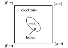
FIG. 1.: A small Fermi surface consisting of a hole pocket centered around $(\pi/2,\pi/2)$.

Whether this idea is fully consistent with the observations is still a subject of debate. If pockets exist, then one should observe two Fermi surface crossings along the zone diagonal. Kendziora et al. argued that they did observe two crossings in their measurements on $30K$ superconductor, and therefore are able to reconstruct the whole pocket [24]. The data by Shen et al. [31] for the most heavily underdoped superconductors also indicate that the maximum in the spectral function first shifts to lower frequencies as one moves from $(0,0)$ to $(\pi/2,\pi/2)$, then disappears before the $(\pi/2,\pi/2)$ point is reached, and then reappears and moves towards higher frequencies as one moves from $(\pi/2,\pi/2)$ to $(\pi,\pi)$. They, however, argued that it is difficult to determine whether the reappearance of the peak between $(\pi/2,\pi/2)$ and $(\pi,\pi)$ is an observation of the second side of the pocket, or whether its reappearance possesses a structural origin [32].

Our interpretation of the photoemission data parallels the one made by Kendziora et al. - we believe that there is substantial evidence that the Fermi surface in the underdoped cuprates does consist of small hole pockets. A natural question one may then ask is whether the formation of pockets is related to the reduction of $T_{c}$. We will argue in the paper that this is, in fact, the case. Specifically, we will argue that in the doping range where the Fermi surface evolves from a large one to a small one, vertex corrections substantially reduce the pairing interaction. How precisely this evolution occurs is the subject of the present paper. Notice that the evolution of the Fermi surface cannot be continuous since the large and small Fermi surfaces are centered around different points in momentum space. In fact, our results show that the Fermi surface evolution should necessary include a Lifshitz-type phase transition in which the topology of the Fermi surface changes.

We conclude the introduction with the discussion of a microscopic model for the cuprates. There are numerous reasons to believe that the low-energy properties of the cuprates are quantitatively captured by the effective 2D one band Hubbard model [33, 34, 35]

$${\cal H}=-\sum_{i,j}t_{i,j}c^{\dagger}_{i,\alpha}c_{j,\alpha}+U\sum_{i}n_{i,\uparrow}n_{i,\downarrow}$$ (3)

Here $\alpha$ is a spin index, $n_{i,\sigma}=c^{\dagger}_{i,\sigma}c_{i,\sigma}$, and $t_{i,j}$ is a hopping integral which we assume to act between nearest and next-nearest neighbors ($t$ and $t^{\prime}$, respectively). By itself, this one-band model is a simplification, since in “first principles” calculations one would start with the three band model for the $CuO_{2}$ unit. However, it is generally accepted that at energies less than about $5eV$ the hybridization between $Cu$ and $O$ orbitals is rather strong, and one can effectively describe the system by a single degree of freedom per $CuO_{2}$ unit [36]. The on-site Coulomb repulsion $U$ which we use in Eq.(3) is close to the actual charge-transfer gap between the unhybridized $Cu$ and $O$ bands which is about $2eV$ .

Furthermore, the Hubbard model contains only electrons but no spins. Spin fluctuations appear in this model as collective modes of fermions. To obtain these modes, one has to sum up the RPA series in the particle-hole channel [37, 38, 39]. As a result of the summation, the product of the two fermionic Green’s functions is replaced by a spin susceptibility whose poles correspond to spin fluctuation modes. The susceptibility thus obtained takes the general form

$$\chi_{ii}({\bf q},\omega)=\frac{\tilde{\chi}_{ii}({\bf q},\omega)}{1-U\tilde{\chi}_{ii}({\bf q},\omega)}$$ (4)

in which $\tilde{\chi}_{ii}(\bf{q},\omega)$ is the irreducible particle-hole susceptibility, and $i=x,y,$ or $z$. Similarly, one can obtain the spin-fermion vertex (i.e., the coupling between two fermions and one spin fluctuation), by starting with the original four-fermion Hubbard interaction term and combining one incoming and one outgoing fermion into the RPA series. One can then introduce an effective model in which fermions and spins are considered as independent degrees of freedom coupled by

$${\cal H}_{int}=g\sum_{{\bf q,k},\alpha,\beta}~{}c^{\dagger}_{{\bf k+q},\alpha}\,{\vec{\sigma}}_{\alpha,\beta}\,c_{{\bf k},\beta}\cdot{\vec{S}}_{\bf-q}$$ (5)

where $\sigma_{i}$ are the Pauli matrices, and the spin propagator (i.e. the Fourier transform of the retarded spin-spin correlation function) is the RPA susceptibility $\chi(q,\omega)$. The coupling constant $g$ is equal to $U$ in the RPA approximation. In semi-phenomenological theories, this coupling, however, is considered as some effective input parameter [26]. The argument here is that $g$ can be substantially renormalized from $U$ due to diagrams not included in the RPA series.

The spin-fermion model is a convenient point of departure if one intends to study the effects of spin fluctuations on the electronic spectrum. We point out, however, that this model neglects a direct fermion-fermion interaction. We will see later in this paper that one actually needs this interaction as a necessary term to restore the Ward identities.

The spin-fermion model can be further simplified if one assumes some phenomenological form for the full spin susceptibility rather than computing it in the RPA approximation. This procedure can partly be justified. The point is that only the imaginary part of the irreducible particle-hole susceptibility comes from an integration near the Fermi surface where the fermionic Green’s function is known on general grounds. The computation of the real part of $\chi(q,\omega)$, on the other hand, involves an integration over regions far from the Fermi surface. In these regions, the actual fermionic propagators can differ substantially from their values for the noninteracting fermions. This in turn implies that the RPA approximation may be insufficient, and a phenomenological form of $\chi$ with the parameters deduced from the experimental data might be more appropriate.

We now briefly discuss the phenomenological form of the susceptibility. One can argue quite generally that in the vicinity of the antiferromagnetic phase, the full spin susceptibility behaves as [40]

$$\chi({\bf{q}},\omega)=\frac{\chi_{\bf Q}}{1+({\bf q}-{\bf Q})^{2}\xi^{2}-i\omega/\omega_{sf}-\omega^{2}\xi^{2}/c_{sw}^{2}}$$ (6)

where $\chi_{\bf Q}=\alpha\xi^{2}$, $\xi$ is the correlation length (measured in units of a lattice constant), $c_{sw}$ is the spin-wave velocity, and $\omega_{sf}=c^{2}_{sw}/2\xi^{2}\gamma$ where $\gamma$ is a spin damping rate. The parameters in the phenomenological susceptibility can be inferred from comparison to NMR and neutron scattering data, as it was demonstrated by Millis, Monien and Pines [40]. The choice of $\alpha$ is indeed arbitrary as it can be absorbed into the coupling constant. Furthermore, as we said above, $\omega_{sf}$ can be computed in an arbitrary Fermi liquid provided that the spin-fermion coupling is not too strong. In fact, a comparison of the calculated (within the above framework) and measured $\omega_{sf}$ yields an information about the value of the quasiparticle residue at the Fermi surface in optimally doped cuprates [41].

In the further discussion, we will consider both Hubbard and effective spin-fermion models. In the next section, we review the large $U$ spin-density-wave approach for a magnetically ordered state at low doping, and show that in the presence of long-range order, the full vertex, $g_{eff}(k)$, in fact vanishes at the antiferromagnetic momentum $k=Q$. Simultaneously, the hole Fermi surface consists of four small pockets. We then argue that both of these features should survive when the system looses long-range order, and disappear only at much larger doping concentrations when the system effectively looses its short-range magnetic order. In Sec III B we study the effective model which reproduces the evolution from a large to a small Fermi surface as the strength of the spin-fermion coupling increases. In Sec III D we compute the corrections to the spin-fermion vertex and show that these corrections substantially reduce the vertex for the range of couplings when the Fermi surface has a small area. Finally, in Sec. IV we state our conclusions and point to unresolved issues.

II Ordered state

We begin our discussion with the magnetically-ordered state. Our emphasis here will be to obtain the form of the spin-fermion interaction vertex, and the shape and the area of the quasiparticle Fermi surface.

A straightforward way to study the ordered state is to apply a spin-density-wave (SDW) formalism [38, 42]. Suppose that the system possesses a commensurate antiferromagnetic order in the ground state. Then the $z-$component of the spin-density operator, ${\vec{S}}(q)=(1/2)\sum_{k}c^{\dagger}_{k+q,\alpha}{\vec{\sigma}}_{\alpha,\beta}c_{k,\beta}$, has a nonzero expectation value at $q=Q=(\pi,\pi)$. In the SDW approach, one uses the relation $\langle\sum_{k}c^{\dagger}_{k+Q,\uparrow}c_{k,\uparrow}\rangle=-\langle\sum_{k}c^{\dagger}_{k+Q,\downarrow}c_{k,\downarrow}\rangle=\langle S_{z}\rangle$ to decouple the quartic term in Eq.(3). The truncated Hamiltonian is then diagonalized by a Bogoliubov transformation to new quasiparticle operators

$$c_{k,\sigma} = u_{k}a_{k,\sigma}+v_{k}b_{k,\sigma},$$ (7)

$$c_{k+Q,\sigma} = sgn(\sigma)(u_{k}b_{k,\sigma}-v_{k}a_{k,\sigma}),$$ (8)

where the fermionic Bogolyubov coefficients are

$$u_{k}=\sqrt{{1\over 2}\left(1+{\epsilon^{(-)}_{k}\over E_{k}}\right)},~{}~{}v_{k}=\sqrt{{1\over 2}\left(1-{\epsilon^{(-)}_{k}\over E_{k}}\right)}.$$ (9)

Here $\epsilon^{(-)}_{k}=(\epsilon_{k}-\epsilon_{k+Q})/2$, $\epsilon_{k}=-2t(\cos k_{x}+\cos k_{y})-4t^{\prime}\cos k_{x}\cos k_{y}$ is the single particle dispersion, and $E_{k}=\sqrt{(\epsilon^{(-)}_{k})^{2}+\Delta^{2}}$, where $\Delta=U\langle S_{z}\rangle$. In the cuprates, “first-principle” calculations yield $t\sim 0.3eV$ and $t^{\prime}\sim-0.06eV$ [43]. Note that $\epsilon^{(-)}_{k}$ only contains $t$, and, hence, the Bogoliubov coefficients do not depend on $t^{\prime}$. The self-consistency condition for $\Delta$ has the simple form $1/U=\sum_{k}1/E^{-}_{k}$, where the summation runs over all occupied states in the magnetic Brillouin zone.

The diagonalization using (8) yields two bands of electronic states (the conduction and valence bands) with a gap $2\Delta\sim U$ in the strong coupling limit ($U\gg t,t^{\prime}$):

$${\cal H}={\sum_{k\sigma}}^{\prime}E^{c}_{k}a^{\dagger}_{k\sigma}a_{k\sigma}-E^{v}_{k}b^{\dagger}_{k\sigma}b_{k\sigma},$$ (10)

where $E^{c,v}_{k}=E_{k}\pm\epsilon^{(+)}_{k}$, $\epsilon^{(+)}_{k}=(\epsilon_{k}+\epsilon_{k+Q})/2$, and the prime restricts the summation to the magnetic Brillouin zone. We can further expand under the square root and obtain $E^{c,d}_{k}=\Delta+J(\cos k_{x}+\cos k_{y})^{2}\mp 4t^{\prime}\cos k_{x}\cos k_{y}$, where $J=4t^{2}/U$ is the magnetic exchange integral.

It is also instructive to present the expression for the fermionic Green’s function. It now has two poles at $\Omega={\bar{E}}^{c,v}_{k}$ (${\bar{E}}=E-\mu$, where $\mu$ is the chemical potential), and vanishes at $\Omega=\epsilon_{k+Q}$. Namely, we have

$$G(k,\Omega)=\frac{u^{2}_{k}}{\Omega-\bar{E}^{c}_{k}}+\frac{v^{2}_{k}}{\Omega-\bar{E}^{v}_{k}}~{}=~{}\frac{\Omega-\bar{\epsilon}_{k+Q}}{(\Omega-\bar{E}^{c}_{k})(\Omega-\bar{E}^{v}_{k})}$$ (11)

Consider now how the Fermi surface evolves as $<S_{z}>$ and, hence, $\Delta$ increases. Suppose that we fix the doping concentration at some small but finite level and increase $\Delta$ from zero to the strong coupling value $\Delta\sim U$. For $\Delta=0$, the Fermi surface for holes has the form shown in Fig 2a - it is centered at $(\pi,\pi)$ and encloses the area which is slightly larger than half of the Brillouin zone, in accordance with the Luttinger theorem.

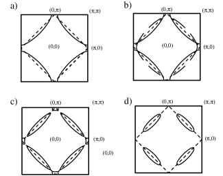
FIG. 2.: Schematic evolution of the Fermi surface with the SDW gap $\Delta$ in the ordered phase of the $t-t^{\prime}$ Hubbard model. We set $t^{\prime}=-0.2t$. For $\Delta=0$ (a) the Fermi surface is large and centered around $(\pi,\pi)$. For $\Delta=0^{+}$ (b) additional pieces of the Fermi surface appear, which are the images of the original Fermi surface shifted by $(\pm\pi,\pm\pi)$. For intermediate $\Delta$ (c) one observes hole and electron pockets around $(\pi/2,\pi/2)$ and $(0,\pi)$, respectively. For large $\Delta$ (d) the Fermi surface just consists of hole pockets centered around $(\pi/2,\pi/2)$. The dashed line indicates the boundary of the magnetic Brillouin zone.

Switching on an infinitesimally small $\Delta$ doubles the unit cell in real space. As a result, the electronic spectrum acquires an extra branch which is just the image of the original dispersion but shifted by Q (see Fig. 3).

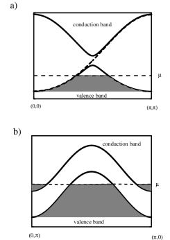
FIG. 3.: The electronic spectrum along the $(0,0)-(\pi,\pi)$ direction (a) and the $(0,\pi)-(\pi,0)$ direction (b) for intermediate $\Delta$ (see Fig.2c). The shaded area corresponds to the filled electronic states. Note the presence of electron pockets around $(0,\pi)$ and $(\pi,0)$. The dashed line in (a) is the quasiparticle spectrum for $\Delta=0$.

The same also happens with the Fermi surface - it acquires extra pieces because a Fermi surface crossing at $k$ necessarily implies one at $k+Q$ (Fig. 2b). The subsequent evolution of the Fermi surface proceeds as is shown in Fig. 2c,d. The details of this evolution are model dependent and therefore are not that relevant. An essential point is that, at large $\Delta$, valence and conduction bands are well separated, and $u_{k}^{2},~{}v^{2}_{k}\approx 1/2$, i.e., $Z\approx 1/2$ for all momenta. Since a summation of the electronic states with quasiparticle residue $Z=1/2$ over the full Brillouin zone gives the same result as a summation of the states with residue $Z=1$ over half of the Brillouin zone, nearly all states in the valence band are occupied, except for a fraction, which is proportional to the doping concentration measured from half filling. This in turn means that the hole Fermi surface should be small and centered around the minimum of $E^{v}_{k}$. For negative $t^{\prime}$ which we only consider here, this minimum is located at $(\pi/2,\pi/2)$ [44, 45] (see Fig. 2d). The area of this small, pocket-like Fermi surface can be obtained either by modifying Luttinger’s arguments to account for the existence of both, two poles and a vanishing numerator in the Green’s function, or by a direct computation of the particle density $N/V$. Performing this computation, we obtain

$$x=S_{hole}-S_{elect}$$ (12)

where $S_{hole}$ and $S_{electr}$ are the closed areas of hole pockets and doubly occupied electronic states (the latter appear at intermediate stages of the Fermi-surface evolution, see Figs. 2c and 3b). At strong coupling $(\Delta\sim U\gg t)$, the doubly occupied electron states disappear and we have $S_{hole}=x$.

We now proceed with the computations of the spin-fermion vertices. In the SDW formalism, the low-energy spin fluctuations (magnons) are collective modes in the transverse spin channel. Consequently, they correspond to the poles of the transverse spin susceptibility. The latter is given in the SDW theory by the series of ladder diagrams. Consider first the strong-coupling limit at half-filling. Then each ladder can only consist of conduction and valence fermions. Since the unit cell is doubled due to the presence of the antiferromagnetic long range order, we have two susceptibilities — one with zero transferred momentum, and one with the momentum transfer ${\bf Q}=(\pi,\pi)$. The explicit forms of these susceptibilities are [38]

$$\chi^{\pm}(q,q,\omega)=-S~{}\sqrt{1-\gamma_{q}\over{1+\gamma_{q}}}~{}\left[\frac{1}{\omega-\Omega_{q}+i\delta}-\frac{1}{\omega+\Omega_{q}-i\delta}\right],$$ (13)

$$\chi^{\pm}(q,q+Q,\omega)=-S~{}~{}\left[\frac{1}{\omega-\Omega_{q}+i\delta}+\frac{1}{\omega+\Omega_{q}-i\delta}\right].$$ (14)

Here $\Omega_{q}=4JS\sqrt{1-\gamma_{q}^{2}}$ is the magnon frequency.

Further, a sequence of bubble diagrams can be viewed as an effective interaction between two fermions mediated by the exchange of a spin-wave. The spin-wave propagators are $i\langle Te_{q}(t)e^{\dagger}_{q}(0)\rangle_{\omega}=(\Omega_{q}-\omega-i\delta)^{-1}$ and $i\langle Te^{\dagger}_{q}(t)e_{q}(0)\rangle_{\omega}=(\Omega_{q}+\omega-i\delta)^{-1}$, where $e^{\dagger}_{q}(e_{q})$ are the boson creation (annihilation) operators, subindex $\omega$ implies Fourier transform, and the momentum $\bf q$ runs over the whole Brillouin zone. A simple experimentation then shows that the form of the two susceptibilities are reproduced if one chooses the following Hamiltonian for the interaction between the original fermionic operators and the magnons [38]:

$$H_{el-mag} = U~{}{\sum_{k}}^{\prime}{\sum_{q}}~{}\Big{[}\eta_{q}c^{\dagger}_{k+q,\alpha}c_{k,\beta}(e^{\dagger}_{-q}+e_{q})$$ (15)

$$+ ~{}{\bar{\eta}}_{q}c^{\dagger}_{k+q,\alpha}c_{k+Q,\beta}(e^{\dagger}_{-q}-e_{q})\Big{]}\delta_{\alpha,-\beta}.$$ (16)

where

$$\eta_{q}=\frac{1}{\sqrt{2}}\left(\frac{1-\gamma_{q}}{1+\gamma_{q}}\right)^{1/4},~{}~{}{\overline{\eta}}_{q}=\frac{1}{\sqrt{2}}\left(\frac{1+\gamma_{q}}{1-\gamma_{q}}\right)^{1/4}.$$ (17)

Performing now the above Bogolyubov transformation, we obtain the Hamiltonian for the interaction between the magnons and the conduction and valence band fermions

$$H_{el-mag} = ~{}{\sum_{k}}^{\prime}{\sum_{q}}~{}\Big{[}a^{\dagger}_{i\alpha k}a_{i\beta,k+q}e^{\dagger}_{q}~{}\Phi_{aa}(k,q)$$ (18)

$$+ b^{\dagger}_{i\alpha k}b_{i\beta,k+q}e^{\dagger}_{q}~{}\Phi_{bb}(k,q)+a^{\dagger}_{i\alpha k}b_{i\beta,k+q}e^{\dagger}_{q}~{}\Phi_{ab}(k,q)$$ (19)

$$+ b^{\dagger}_{i\alpha k}a_{i\beta,k+q}e^{\dagger}_{q}~{}\Phi_{ba}(k,q)+~{}{\rm H.c.}~{}\Big{]}~{}\delta_{\alpha,-\beta}.$$ (20)

The vertex functions are given by

$$\Phi_{aa,bb}(k,q) = U\Big{[}\pm\Big{(}u_{k}u_{k+q}-v_{k}v_{k+q}\Big{)}\eta_{q}+\Big{(}u_{k}v_{k+q}$$ (21)

$$- v_{k}u_{k+q}\Big{)}{\overline{\eta}}_{q}\Big{]},$$ (22)

$$\Phi_{ab,ba}(k,q) = U~{}\Big{[}\Big{(}u_{k}v_{k+q}+v_{k}u_{k+q}\Big{)}\eta_{q}\mp\Big{(}u_{k}u_{k+q}$$ (23)

$$+ v_{k}v_{k+q}\Big{)}{\overline{\eta}}_{q}\Big{]}$$ (24)

In the strong coupling limit which we actually study now, they reduce to

$$\Phi_{aa,bb}(k,q) = \left[\pm\Big{(}\epsilon^{(-)}_{k}+\epsilon^{(-)}_{k+q}\Big{)}\eta_{q}+\Big{(}\epsilon^{(-)}_{k}-\epsilon^{(-)}_{k+q}\Big{)}{\overline{\eta}}_{q}\right],$$ (25)

$$\Phi_{ab,ba}(k,q) = U~{}\left[\eta_{q}\mp{\overline{\eta}}_{q}\right].$$ (26)

We see that there are two types of vertices: $\Phi_{ab,ba}$ which describes the interaction between conduction and valence fermions, and $\Phi_{aa,bb}$ which involves either valence or conduction fermions. The first vertex is virtually not renormalized by Bogolyubov coefficients. However, at large $\Delta$, it involves high-energy conduction fermions and therefore can be omitted. The second vertex is the one relevant for the pairing mechanism since slightly away from half-filling, both valence fermions can simultaneously be on the Fermi surface. We see that this vertex is substantially reduced at large coupling - it is of the order of the hopping integral rather than of the order of $U$. Moreover, it is easy to verify that $\Phi_{bb}$ in fact vanishes as the magnon momentum approaches $Q$. For $q$ close to $Q$, we have, expanding Eq.(26), $\Phi_{bb}\propto t|q-Q|^{1/2}$. The vanishing of $\Phi_{bb}$ at $q=Q$ is a consequence of the Adler principle: in the ordered state, magnons are Goldstone bosons and their interaction with other degrees of freedom should vanish at the ordering momentum to preserve the Goldstone mode to all orders in perturbation theory. Note in this regard that the vertex which includes conduction and valence fermions should not be included into the corrections to the spin propagator. Indeed, this vertex is already used in the RPA series which yields the spin susceptibility presented in Eq.(14), and to include it into the corrections will just be double counting of the same diagrams. From this perspective, the fact that $\Phi_{ab,ba}$ does not vanish for $q=Q$ is not a violation of the Adler principle.

We now construct the effective vertex for the spin-fermion model. Since the factors $\eta_{q}$ and $\bar{\eta}_{q}$ are derived from the spin susceptibility, we have to absorb them into $S_{q}$. Actually, only $\eta_{q}$ is relevant as it diverges at $q=Q$. Eliminating this factor in $\Phi_{bb}$, and substituting $U$ by the bare coupling constant $g$, we find that the effective spin-fermion interaction behaves as

$$g_{eff}=g~{}\left(u_{k}u_{k+q}-v_{k}v_{k+q}\right)\propto t|q-Q|.$$ (27)

This result was first obtained by Schrieffer [46]. We see that as long as one can keep the conduction fermions far away from the Fermi surface (which is the case at strong couplings), the effective pairing interaction between fermions is substantially reduced by a vertex renormalization [47]. Consider now the full static interaction between fermions mediated by spin fluctuations. It is given by $\Gamma(q)=(g_{eff}(q))^{2}~{}\chi(q)$. Since $\chi(q)\propto(q-Q)^{-2}$ and $g_{eff}(q)\propto|q-Q|$, $\Gamma(q)$ tends to a positive constant as $q$ approaches $Q$. On the other hand, however, we would need a substantial enhancement of the interaction near $Q$ for the appearance of $d-$wave superconductivity. We see, therefore, that the presence of a long-range order actually excludes the occurrence of $d-$wave superconductivity at large $U$. In the next section we will study in detail what happens when the sublattice magnetization decreases and the mean-field gap, $\Delta=U<S_{z}>$, becomes smaller than the fermionic bandwidth despite a large $U$. At this point, however, we merely emphasize the correlation between the relevance of vertex corrections and the shape of the Fermi surface, namely, that when the Fermi surface consists of small hole pockets, vertex corrections are relevant and the full vertex is much smaller than the bare one.

A Fluctuation effects

Our next goal is to study how fluctuations modify this simple mean-field picture. We will show that the mean-field form of the quasiparticle dispersion remains qualitatively (and even partly quantitatively) correct even at strong couplings though there is a substantial shift of the spectral weight from the coherent part of the spectral function to the incoherent part which stretches upto frequencies of a few $t$. At the same time, the relation $\Delta=U<S_{z}>$ does not survive beyond mean-field theory, and the strong-coupling, SDW-like form of the quasiparticle dispersion with a gap between two bands holds even when the system looses long-range antiferromagnetic order. More specifically, we will show that there exist two different self-energy corrections. One self-energy correction is strong but nonsingular. It gives rise to a shift of the spectral weight towards the incoherent part of the spectral function, but preserves coherent excitations on the scale of $J$. The second correction renormalizes the gap but does not change the form of the quasiparticle Green’s function. This correction is however singular for vanishing $<S_{z}>$ and breaks the relation between $\Delta$ and $<S_{z}>$ such that the gap survives and remains of $O(U)$ when $<S_{z}>$ vanishes. To perform a perturbative expansion around the mean-field SDW state, we need an expansion parameter. Obviously, an expansion in $U$ will not work as we assume that $U\gg t$. There exists, however, a formal way to make the mean-field theory exact - one should extend the original Hubbard model to a large number of orbitals at a given site, $n_{c}=2S$, and perform an expansion in $1/S$ [44, 48]. The $S=\infty$ limit corresponds to the mean-field solution, and all corrections are in powers of $1/S$. The mean-field result for the spectrum is the same as in Eq.(10) apart from the extra factor of $2S$ (we also have to redefine ${\bar{t}}=t/2S$ as $t$ now scales with $S$).

Consider now the lowest-order self-energy correction to the propagator of the valence fermions. To first order in $1/S$, there are two self-energy diagrams, one involves only valence fermions, and the other involves both, valence and conduction fermions (Fig. 4).

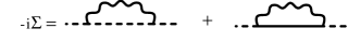
FIG. 4.: The lowest order self-energy corrections for the valence fermions. The solid and dashed lines are the bare propagators for the conduction and valence fermions, respectively. The wavy line describes transverse spin fluctuations.

In the first diagram, the vertex is reduced from $U$ to $O(t)$ and vanishes at $q=Q$. Numerically, however, this diagram yields large corrections since the large term, $\Delta\sim US$, in the energy denominator is cancelled out because both fermions are in the valence band. The denominator is then of the order of $O(JS)$. As a result, the self-energy correction from this diagram scales as $O({\bar{t}}^{2}/JS)=O(U)$ and obviously contains some dispersion at this scale [44]. At the same time, the bare dispersion is at the scale of $JS$. We see that one clearly needs more than just smallness of $1/S$ to make perturbation theory work - the ratio $U/JS$ should be small too. This last assumption is not justified for high-$T_{c}$ materials where $(U/JS)$ is typically of the order of $\sim 20-30$.

We recently considered this diagram in detail and performed self-consistent calculations of the electronic dispersion assuming that $1/S\ll 1$ but also $U/JS\gg 1$ [49]. One can show that in this limit one can neglect vertex corrections but has to include the whole series of rainbow diagrams for self-energy corrections [50]. This corresponds to the insertion of the full Green’s function into the internal fermionic line in Fig.4. The self-consistency equation for $G(k,\omega)$ then takes the following form:

$$G^{-1}(k,\omega) = \omega+\epsilon_{k}^{MF}$$ (29)

$$\;-\int{d^{2}q\Psi(k,q)G(k+q,\omega+\Omega_{q})}$$

where

$$\epsilon_{k}^{MF}=\Delta+2JS(\cos k_{x}+\cos k_{y})^{2}-4t^{\prime}\cos k_{x}\cos k_{y}$$

is the mean-field dispersion and

$$\Psi(k,q) = 32\bar{t}^{2}S\Big{[}\nu_{k}^{2}+\nu_{k+q}^{2}-2\nu_{k}\nu_{q}\nu_{k+q}$$

$$+ \sqrt{1-\nu_{q}^{2}}(\nu_{k+q}-\nu_{k})\Big{]}/\sqrt{1-\nu_{q}^{2}}$$

Note that Eq.(29) is an integral equation in both momentum and frequency space.

The form of the quasiparticle dispersion in the ordered phase is interesting in its own because of recent photoemission data on $Sr_{2}CuO_{2}Cl_{2}$ [51, 52]. These data show that (i) the valence band dispersion is isotropic near the top of the band which is at $(\pi/2,\pi/2)$, and relatively well described by the mean-field formula with $t^{\prime}=-0.5J$, but (ii) coherent excitations exist only near $(\pi/2,\pi/2)$. As soon as one deviates from this point, the width of the quasiparticle peak rapidly increases, and at the scale of $2J$, the excitations become mostly incoherent. Monte-Carlo and finite cluster simulations in the insulating phase have similarly demonstrated that there exist coherent excitations at scales smaller than $2J$, but also incoherent excitations which stretch upto a few $t$ [53, 54].

Our analytical results are consistent with the experimental data and with the numerical simulations. We first discuss the critical value of $\omega$ for which one first observes a finite imaginary part of $G(k,\omega)$, or equivalently, the onset of a finite density of states (DOS) [55]. On a mean-field level, this happens on the scale of $\omega+\Delta=O(JS)$. The analysis of Eq.(29) shows, however, that the onset of a DOS actually occurs at the much larger scale of $\omega+\Delta=O({\bar{t}}\sqrt{S})$. At these energy scales, the frequency shift due to $\Omega_{q}$ on the r.h.s. of Eq.(29) can be neglected, and we just have to solve an integral equation in momentum space. Doing this by standard means, we obtain that a nonzero DOS appears at

$$\omega_{cr}+\Delta=\pm 4.2\bar{t}\sqrt{2S}.$$

In the vicinity of $\omega_{cr}$, the DOS behaves as $N(\omega)\sim\sqrt{|\omega-\omega_{cr}|}$. We see, therefore, that the incoherent part of the Green’s function stretches upto scales comparable to the original fermionic bandwidth.
Another important issue is the form of the quasiparticle Green’s function at $|\omega_{cr}-\omega|\leq JS$, where one can show that the contribution from the magnon dispersion in fact cannot be neglected. In addition, photoemission experiments have shown strong evidence for coherent fermionic excitations in this region. We therefore assumed the following trial form of the fermionic Green’s function in the vicinity of $\omega_{cr}$

$$G(k,\omega)={Z_{k}\over\omega-\omega_{cr}+A(k)-i\gamma(\omega-\omega_{cr})^{2}}$$ (30)

Performing self-consistent computations in this region, we found [49] that the quasiparticle residue is indeed small, $Z\sim O(J\sqrt{S}/t)\ll 1$. Analogous result has been obtained by Kane, Lee and Read [50]. At the same time, $A(k)$ is zero right at $(\pi/2,\pi/2)$ and scales quadratically with the deviation from this point. The scale for the coherent dispersion is $JS$ - the same as for the mean-field solution. Even more, we recovered the isotropic dispersion near $(\pi/2,\pi/2)$, namely $A(k)=2JS\tilde{k}^{2},\quad{\tilde{k}}=(\pi/2,\pi/2)-{k}$, and obtained the same bandwidth $2J$ as in the experimental data. For the damping rate we found $\gamma\sim 1/JS$. It follows from our results that there exists just one typical energy scale $JS$ which separates coherent excitations at smaller energies and incoherent excitations at higher energies (see Fig.5).

FIG. 5.: Schematic form of the total DOS resulting from the self-consistent solution of Eq.29. $W$ is the bandwidth for free fermions.

It is essential that this holds in the strong-coupling limit $t\gg J\sqrt{S}$ when the quasiparticle residue $Z\ll 1$, and the mean-field dispersion is completely overshadowed by self-energy corrections. In this respect, the existence of coherent excitations at the scales of $JS$ turns out to be an intrinsic property of the Hubbard model and not the result of a mean-field approximation. Moreover, since the vertex does not depend on $t^{\prime}$, the strong-coupling results are independent of the $t^{\prime}/J$ ratio, contrary to the mean-field dispersion [56]. Notice also that the dominant corrections due to valence-valence vertex come from short-range spin fluctuations. The contribution from long-range fluctuations with $q\approx Q$ is reduced due to a vanishing vertex at $q=Q$. In other words, the valence-valence diagrams are certainly non-singular. Not surprisingly then, these corrections can reduce the coherent part of the quasiparticle dispersion but cannot qualitatively change the mean-field description. For the sake of simplicity, we will just neglect these corrections for the rest of the paper.

We will now discuss the self-energy correction which involves both conduction and valence fermions. Here the vertex is of the order of $U$, but the energy denominator scales as $US$. As a result, one obtains a momentum-independent correction to the gap, and also (doing expansion in $J/U$ and in $\omega/U$, where $\omega$ is the external frequency) a correction to the dispersion on the scale of $O(J)$. The latter is nothing but the conventional $1/S$ correction to the mean-field dispersion which is obviously small at large $S$. In other words, the inclusion of the self-energy diagram with valence and conduction fermions leaves the structure of the quasiparticle Green’s function unchanged, but renormalizes the gap. It is essential, however, that the gap renormalization can be made singular when $<S_{z}>$ vanishes. The easiest way to see this is to consider what happens at infinitesimally small temperatures in $2D$. The Mermin-Wagner theorem tells us that immediately as the temperature becomes finite, the long-range order should disappear. In perturbation theory, the onset of this effect is the appearance of logarithmically divergent correction which scales as $T\log L$ where $L$ is the system size. We evaluated the self-energy correction at $T=0^{+}$ and obtained

$$\Sigma=-U~{}{1\over N}\sum_{q}{1-\sqrt{1-\nu^{2}_{q}}\over\sqrt{1-\nu^{2}_{q}}}~{}(1+2n^{b}_{q})$$ (31)

where $n^{b}_{q}=(exp(\Omega_{q}/T)-1)^{-1}$ is the Bose distribution function. At any finite $T$, $\Sigma$ is logarithmically divergent: $\Sigma\propto T\int d^{2}q/q^{2}\sim T\log L$. If this were the only correction, the mean-field description would be completely destroyed. However, there exist another logarithmically divergent diagram which cancels the contribution from $\Sigma$. The point is that the mean-field expression for the gap $\Delta_{MF}=U<S_{z}>$ contains the exact sublattice magnetization. On the mean-field level, one has (at large $U$), $<S_{z}>\approx S$. When $T$ becomes nonzero, $<S_{z}>$ also acquires a logarithmically divergent correction which involves the valence-conduction vertex (see Fig. 6b).

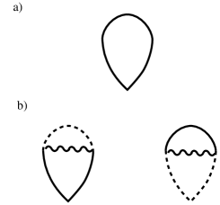
FIG. 6.: The loop diagrams for $<S_{z}>$. The diagram in (a) represents $<S_{z}>/S$ on the mean-field level while those in (b) correspond to the lowest order corrections to $<S_{z}>/S$ due to the exchange of transverse fluctuations.

In analytical form, we have

$$\delta(<S_{z}>)=-{1\over N}\sum_{q}{1-\sqrt{1-\nu^{2}_{q}}\over\sqrt{1-\nu^{2}_{q}}}~{}(1+2n^{b}_{q})$$ (32)

Combining these two terms, we find that the logarithmically divergent corrections to $\Delta$ are cancelled out. As a result, $\Delta$ remains finite even when the long-range order disappears. Moreover, a comparison of Eq.(31) and Eq.(32) shows that the gap remains exactly equal to $US$ in the large $U$ limit.

By itself, this result is not surprising since at large $U$, the valence and conduction bands are nothing but the lower and upper Hubbard bands, respectively. In the near atomic limit, the gap between the two bands should be equal to $U$ (for $S=1/2$) upto corrections of $O((t/U)^{2})$ independent of whether or not the system is ordered. We extended our calculations to analyze the form of the full quasiparticle Green’s function and found that not only $\Delta$ but also $G_{full}(k,\omega)$ is free from logarithmical singularities and therefore does not undergo sharp changes when one looses long-range order due to singular thermal fluctuations. In other words, we found that the SDW structure of the electronic states with two coherent bands separated by a large gap $\approx U$ survives when the system looses long-range order. We remind that the key features of the SDW state at large $U$ are the small Fermi surface and a strong reduction of the pairing vertex. We see that both features may exist even without a long-range order. The interesting issue then arises how the system evolves with doping in the paramagnetic state and how it eventually restores a large Fermi surface and a momentum independent vertex function. Notice that without strong magnetic fluctuations, the two bands which emerge from the Hubbard levels are likely to be mostly incoherent, and there also appears, at finite $t$, a coherent band at about $U/2$. This was found in the infinite-$D$ studies of the Hubbard-model [57]. Before we proceed to the discussion of the Fermi surface evolution, we consider another, complimentary approach to the ordered phase, introduced by Kampf and Schrieffer [58]. They demonstrated that one can obtain a mean-field SDW solution in the spin-fermion model without introducing a condensate, but by assuming that the longitudinal spin susceptibility has a $\delta-$functional peak at zero frequency and momentum transfer $Q$: $\chi_{l}(q,\omega)=(1/4)~{}\delta(\omega)\delta(q-Q)$. To recover the mean-field SDW result within the spin-fermion model one has to compute the lowest-order self-energy diagram which includes only the exchange of longitudinal fluctuations. This diagram is shown in Fig.7c.

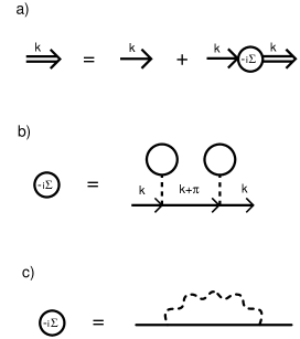
FIG. 7.: (a) The Gorkov equation for the normal Green’s function for the SDW state. The single and double solid lines correspond to the bare and full fermionic propagators. (b) The self-energy diagram which includes two anomalous loops The straight dashed line represents the interaction term $U$. (c) Formal representation of the same diagram as in (b) with the exchange of a $\delta-$functional longitudinal spin fluctuations.

We then obtain

$$\Sigma(k,\omega)=\frac{g^{2}}{4}~{}\frac{1}{\omega-\bar{\epsilon}_{k+Q}}$$ (33)

where, as before, $\bar{\epsilon}_{k}=\epsilon_{k}-\mu.$ Substituting this diagram into the Dyson equation, one immediately recovers the mean-field SDW result for the spectrum with $g$ being the equivalent of $U$.

Furthermore, one can also reproduce the correct form of the vertex between fermions and transverse spin fluctuations. The bare vertex is equal to $g$. To restore the correct mean-field form of the full vertex, one has to include the second-order vertex renormalization due to longitudinal spin fluctuations. The second order vertex correction is given by the diagram in Fig 8.

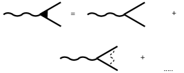
FIG. 8.: The diagrammatic representation for the full vertex (filled triangle) between transverse spin fluctuations and fermions in the ordered state. The solid and dashed wavy lines correspond to the transverse and longitudinal spin fluctuations, respectively. The solid straight lines are the bare fermion Green’s functions. Note that the momenta of the incoming and outgoing fermions differ by $Q=(\pi,\pi)$.

The evaluation of this diagram is straightforward, and we obtain

$$\delta g=-\frac{g^{3}}{4}~{}\frac{1}{(\omega-{\bar{\epsilon}}_{k+Q})(\omega+\Omega-{\bar{\epsilon}}_{k+Q+q})}$$ (34)

where $q$ is the magnon momentum, and $\omega$ and $\Omega$ are the external fermionic and magnon frequencies, respectively. Combining this result with $g$, we find the total vertex in the form

$$g_{tot}=g~{}\frac{(\omega-{\bar{\epsilon}}_{k+Q})(\omega+\Omega-{\bar{\epsilon}}_{k+q+Q})-(g/2)^{2}}{(\omega-{\bar{\epsilon}}_{k})(\omega+\Omega-{\bar{\epsilon}}_{k+q+Q})}$$ (35)

For the vertex which involves only valence fermions, we have at the mass surface, $\omega=-E^{v}_{k},~{}\omega+\Omega=-E^{v}_{k+q}$. Substituting this into Eq.(35) and doing elementary manipulations, we obtain the same expression as in Eq.(27). This result has also been obtained by Schrieffer [46].

One may wonder what happens with the higher-order self-energy and vertex corrections. In fact, they simply do not exist. The reason is that the use of the $\delta-$functional form of the longitudinal susceptibility is just a way to reexpress the mean-field decoupling without formally introducing the condensate. Specifically, one can rewrite the Gorkov equations for the SDW state by introducing the condensate, but without formally introducing the anomalous Green’s function, as is shown in Fig. 7. The self-energy diagram obtained in this way is shown in Fig. 7b. We can now formally combine the two anomalous loops into the $\delta-$functional longitudinal susceptibility in which case we obtain the diagram in Fig. 7c. However, this is just a formal way to reexpress the standard mean-field results. Still, any inclusion of the renormalization of the internal fermionic line in fact means that one inserts more pairs of anomalous loops into the self-energy, which one cannot do since this will render $\Sigma$ reduceable.

The Kampf-Schrieffer approach has the advantage over the conventional SDW decoupling in that it can straightforwardly be extended to the region where long-range order is not present, but where strong antiferromagnetic fluctuations exist, i.e. where the correlation length is large, and the spin susceptibility is strongly peaked, but not divergent, at zero frequency and at the antiferromagnetic momentum. These are the basic assumptions for a nearly antiferromagnetic Fermi-liquid which we are going to study in the following section.

III The nearly antiferromagnetic Fermi-Liquid

A Transverse and longitudinal modes

At first glance, the calculations performed in the ordered phase using the spin-fermion model can be directly extended to the case of a “nearly” $\delta$-functional form of the spin susceptibility in the disordered phase. However, this extension requires some care since in the disordered phase, one no longer can distinguish between transverse and longitudinal fluctuations. Both modes behave in the same way, and both diverge as one approaches the antiferromagnetic transition.

Now, if we apply the second-order diagram to evaluate the Green’s function (see Fig.9a), we do obtain the SDW form of the electronic spectrum as Kampf and Schrieffer have demonstrated, provided that the coupling is larger than the upper cutoff, $\omega_{0}$, in the spin susceptibility.

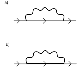
FIG. 9.: (a) The lowest-order self-energy diagram for the spin-fermion model without long-range order. The wavy line describes the exchange of spin fluctuations. All three fluctuation modes contribute equally to the self-energy. (b) The self-energy diagram in the FLEX approximation. The double line describes the full fermionic propagator.

However, because all three modes (two transverse modes and one longitudinal mode) equally contribute to the self-energy, the second-order self-energy at large coupling $g\gg\omega_{0}$ is given by

$$\Sigma_{\alpha}(k,\omega) = g^{2}~{}\sum_{a=1}^{3}\sigma^{a}_{\alpha\beta}\sigma^{a}_{\beta\alpha}\int\chi_{aa}(q,\Omega)G_{0}(k+q,\omega+\Omega)$$ (36)

$$\approx \frac{3}{4}~{}g^{2}~{}G_{0}(k+Q,\omega)$$ (37)

(we normalized $\int\chi_{aa}(q,\Omega)$ to $1/4$). This self-energy yields a “near” SDW solution with the relative corrections of the order $(\omega_{0}/g)^{2}$, but with the gap larger by a factor of $\sqrt{3}$ than the one in the ordered phase (i.e., $\Delta^{2}\approx 3(g/2)^{2}$). At the same time, the vertex correction term at $g\gg\omega_{0}$ does not acquire an extra overall factor:

$$\delta g/g = g^{2}~{}\sum_{a=1}^{3}\sigma^{a}_{\alpha\gamma}\sigma^{b}_{\gamma\delta}\sigma^{a}_{\delta\beta}\int G_{0}(k+p,\omega+\bar{\omega})$$ (40)

$$\times\;G_{0}(k+q+p,\omega+\Omega+\bar{\omega})~{}\chi_{aa}(p,\bar{\omega})\,dp\,d\bar{\omega}$$

$$\approx-(g/2)^{2}~{}G_{0}(k+Q,\omega)~{}G_{0}(k+q+Q,\omega+\Omega)$$

As a result, the relative vertex correction on the mass shell ($\omega\approx-\Delta,G_{0}\approx 1/\Delta$) will scale as $\delta g\approx-g~{}(g/2\Delta)^{2}$ and will only account for a reduction of $g$ by a factor $1/3$. This in turn implies that the full vertex will not vanish for $q=Q$, contrary to what one should expect if the mean-field SDW solution survives the loss of the sublattice magnetization. The reason for this discrepancy is that we have not yet included the counterterm which in the ordered phase cancelled out the correction due to transverse fluctuations thus eliminating two out of the three components of the spin susceptibility in the self-energy diagram. Indeed, if we leave just one component of $\chi$ in Eq.(37), we find for the gap $\Delta\approx(g/2)$ in which case $\delta g\approx-g$ and one recovers the correct form of the vertex.

In order to identify the diagram which eliminates two components of the spin susceptibility in the paramagnetic phase, we go back to the ordered state, reformulate the mean-field SDW theory as a result of the exchange of spin fluctuations and find the diagram which cancels the contribution from the transverse susceptibility. Obviously, this counterdiagram should include a correction to $<S_{z}>$. The corresponding diagram for the Hubbard model is shown in Fig. 10a.

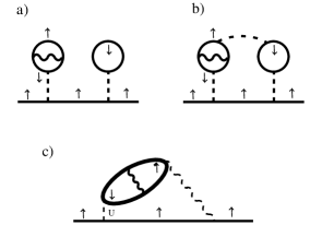
FIG. 10.: The counter diagram which cancels the contribution from the lowest order self-energy term due to transverse spin fluctuations in the ordered state. The transformation from a to c is explained in the text. The solid and dashed lines represent the bare fermionic propagator and the interaction $U$, respectively. The solid and dashed wavy line describe transverse and longitudinal spin fluctuations, respectively. Observe that this diagram still contains the direct fermion-fermion interaction $U$.

Note that the internal lines in the anomalous loop are the full quasiparticle Green’s functions given by Eq.(11). Performing the same manipulations that lead to the exchange of longitudinal fluctuations (i.e., connecting the two anomalous bubbles by $U$ (Fig.10b) and then substituting the single bubble by the full RPA series), we arrive at the diagram shown in Fig. 10c. This diagram includes spin-fermion vertices for the exchange of both, transverse and longitudinal fluctuations, but also the bare Hubbard $U$. The presence of the bare $U$ is crucial - it implies that this diagram cannot be obtained in the pure spin-fermion model since it neglects a direct fermion-fermion interaction. One can easily check that for a $\delta$-functional form of the longitudinal susceptibility this diagram and the second-order diagram with transverse spin exchange cancel each other in the large $U$ limit leaving the diagram with longitudinal spin exchange as the only relevant self-energy diagram.

Suppose now that the long-range order is lost but spin fluctuations are strong. Then our reasoning is the following. Assume first that only one component of the susceptibility should be counted in the self-energy. Then, as we just discussed, we obtain an SDW solution for $g=U\gg\omega_{0}$. We then substitute the SDW form of $G(k,\omega)$ into the remaining part of the self-energy (the same as in Fig.9a, but with only two components of the susceptibility left) and into the fermionic bubble of the diagram in Fig. 10c. Computing the total contribution from these two diagrams we found that this contribution is small compared to the one from Fig. 7c by a factor $(\omega_{0}/g)^{2}$. This in turn justifies the use of only one component of the susceptibility in the second-order self-energy.
Note that at small $g$ the situation is different: the counterdiagram in Fig. 10b is of higher order in $g$ and can be neglected. In this limit, we recover a conventional result of the lowest-order paramagnon theory that all three modes of spin fluctuations contribute to the self-energy.

We now briefly discuss higher order corrections. In the paramagnetic phase, they indeed exist and, moreover, are not small at large $g$. However, extending the same line of reasoning as above to higher-order diagrams, one can easily verify that the higher-order self-energy and vertex corrections nearly cancel each other in the large $g$ limit. For example, the third-order self-energy and vertex correction terms are shown in Fig. 11.

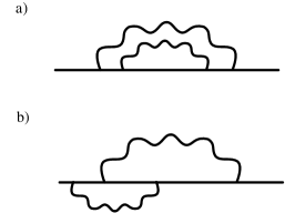
FIG. 11.: Third order diagrams for (a) the self-energy and (b) the vertex correction. At large $g$ these two diagram nearly cancel each other.

Assuming that just one fluctuation mode contributes to the renormalization of the internal fermionic line, we find after simple algebra that the two corrections nearly (to order $(\omega_{0}/g)^{2}$) cancel each other. One, therefore can restrict with only the second-order diagram and hence fully recovers the mean-field SDW solution.

Before we conclude this section we want to comment on what happens if we restrict our calculations to the pure spin-fermion model. In this case each inclusion of the self-energy correction introduces a factor of 3 due to the absence of a counterterm. At the same time, the inclusion of the vertex correction only yields a relative factor of one. This implies that the self-energy corrections are more relevant than the corrections to the vertex. This point can be made rigorous by extending the $SU(2)$ spins to $SU(N)$ and taking the limit of large $N$ [59]. For general $N$, one substitutes the Pauli matrices $\vec{\sigma}$ in (5) by the $(N^{2}-1)$ traceless generators of $SU(N)$. In the large $N$ limit, the vertex corrections are small by a factor of $1/(N^{2}-1)$ and their relative contribution disappears at $N\rightarrow\infty$. At the same time, higher-order self-energy corrections do not contain extra powers of $1/N$ compared to the second-order diagram, and therefore should all be included. The full self-energy correction is then given by a series of rainbow diagrams, which obviously can be reexpressed as a second-order diagram with the full Green’s function for the intermediate fermion (see Fig.9b). This approximation is known as the fluctuation exchange (FLEX) approximation (the fully self-consistent FLEX approximation also uses the full fermionic Green’s functions in the RPA series for the spin susceptibility). The solution of the FLEX equations always yields a large, Luttinger-type Fermi surface with progressively decreasing quasiparticle residue as the spin-fermion coupling increases. We argue that at least in the large coupling limit, this procedure is incomplete because for each inclusion of the rainbow diagram one should also include a counterterm which effectively eliminates $N^{2}-2$ components of the susceptibility out of the self-energy correction. Performing calculations along this line, one indeed recovers the SDW results.

B The model

We now discuss the model we are going to study. In a “first principles” calculation, we would have to consider the Hubbard model. At large $U$, this model contains two peaks in the density of states (the upper and lower Hubbard band) for any doping concentration. Far away from half filling, however, the total spectral weight of the upper band is small, and the excitations in this band are likely to be incoherent. As the system approaches half-filling, the spectral weight is shifted from the lower to the upper band and one gradually recovers the SDW form of the spectrum even before the system becomes magnetically ordered. How this evolution occurs is one of the key issues in understanding the normal state of the cuprates. We have not yet solved this problem in the Hubbard model, instead, we considered the evolution of the spectral function in a toy spin-fermion model. We assume that the density of holes is fixed at some small but finite level, and vary the coupling constant $g$. In doing this, we in fact model the system’s behavior as it approaches half-filling simply because by all accounts, the spin-fermion coupling should increase as the system becomes more “magnetic”.

Further, for any $g$, we compute the self-energy corrections restricting with just one component of the spin susceptibility. The argument here is that, at strong coupling, a counterterm which we discussed in the previous section, cancels out the corrections due to the other two components of the susceptibility. At small couplings, we indeed will miss the overall factor of $3$ in the self-energy, but this does not seem relevant as we do not expect any qualitative changes in the fermionic spectrum. On the other hand, the study of the toy model should give us the answers to two key questions: (i) how does the Fermi surface evolve from a large one, centered at $(\pi,\pi)$, at small couplings to a small one, centered at $(\pi/2,\pi/2)$ at large $g$, and (ii) how does the spin-fermion vertex evolve from a momentum-independent one at small $g$ to one which vanishes at $Q$ (upto $(\omega_{0}/g)^{2}$) terms) at large couplings.

Finally, we assume that the susceptibility has the form of Eq.(6) with some given $\omega_{sf},~{}\xi$ and $c_{sw}$ which do not depend on the strength of the spin-fermion coupling. This is indeed an approximation. When $g$ is large and precursors of the SDW state are already formed, the particle-hole bubbles which constitute the RPA series for the susceptibility should indeed be computed with the full Green’s functions and the full vertices. However, as we will see below, at large $g$, we in fact probe the scales larger than $\omega_{0}$, in which case the structure of $\chi({\bf q},\omega)$ at $\omega<\omega_{0}$ is irrelevant - we only use the fact that the susceptibility obeys the sum rule. At weak coupling, $g<\omega_{0}$, the form of the susceptibility is relevant, but in this limit the real part of the susceptibility is just an input function, independent on $g$, while the imaginary part of $\chi$ can be computed using the bare fermionic Green’s functions and vertices which, in fact, we will do later.

The form of $\chi_{ii}({\bf q},\omega)$ as in Eq.(6) is indeed an expansion near $\omega=0$ and $q=Q$. Meanwhile, $\chi(q,\omega)$ should indeed satisfy the sum rule $\int d\omega\,d^{2}{\bf q}\,\chi_{ii}(q,\omega)=1/4$. To impose the sum rule, one should either add extra terms into Eq.(6) with higher powers of $(q-Q)^{2}$, or impose a cutoff in the momentum integration. For computational purposes, it is easier to impose a cutoff $\omega_{0}$. We have checked that the results for the Fermi-surface evolution practically do not depend on whether we impose a cutoff only in the momentum integration or also in the integration over frequency. In the latter case, however, the computations are much easier to perform and a number of results can be obtained analytically. Below we present the results for the model with a cutoff $\omega_{0}$ in both momentum and frequency.

After presenting the model, we now proceed to our calculations. We will compute the full quasiparticle Green’s function and the full vertex restricting with the second-order diagrams only. Here we apply the same reasoning as before, namely that in both the weak and the strong coupling limit, the relative corrections to the second-order expressions are small and scale as $(g/\omega_{0})^{2}$ and $(\omega_{0}/g)^{2}$, respectively. This implies that the second-order theory will yield a correct limiting behavior at weak and strong couplings. At intermediate couplings, $g\sim\omega_{0}$, higher-order terms are indeed not small. However, even without them, we found in our numerical studies that for intermediate $g$, the solutions for the Green’s function and the vertex strongly depend on the values of $\omega_{sf},\xi$, etc., i.e. the behavior is highly nonuniversal. It is therefore unlikely that the inclusion of higher-order diagrams will give rise to new behavior which is not already present in the second-order theory.

We deem it essential to point out that, though we restrict the corrections to the second-order diagrams only, the computations of $G_{full}(k,\omega)=G_{0}(k,\omega)/(1-\Sigma(k,\omega)G_{0}(k,\omega))$ ($G_{0}$ is the fermionic Green’s function at $g=0$) and the full vertex contain a nonperturbative self-consistency procedure which is necessary to describe a transformation from a large to a small Fermi surface. Namely, we consider the chemical potential $\mu$ as an input parameter in the calculation of the self-energy, and then determine it from the condition that the total density of particles is equal to a given number, $\int d\omega d^{2}k\,G_{full}(k,\omega)=(1-x)/2$. The nonperturbative nature of this procedure appears since the self-energy is not small at large $g$, and one finds a finite region in $(k,\omega)$ space where $\Sigma(k,\omega)G_{0}(k,\omega)>1$ i.e. the perturbative expansion of $G_{full}(k,\omega)$ in powers of $\Sigma$ does not converge. This region, on the other hand, contributes to the density of particles, and this makes the evaluation of $\mu$ a nonperturbative procedure.

We are now ready to present our results. We begin with the self-energy corrections which give rise to the Fermi surface evolution. Some of the results presented in the next subsection have already been reported earlier [60].

C Fermi-surface evolution

As before, we assume that without a spin-fermion interaction, the system behaves as a Fermi-liquid with a large Fermi surface which crosses the magnetic Brillouin zone boundary (see Fig.12a and 13a).

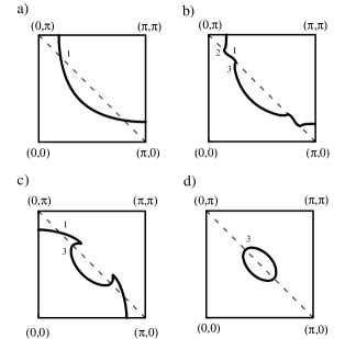
FIG. 12.: The evolution of the hot spots with the coupling strength. For $g<g^{(1)}_{cr}$ (a) there exist only one hot spot; for $g=g^{(1)}_{cr}$ it splits into three (b). As $g$ continues to increase, one progressively looses two of the hot spots (c), and for $g\gg g^{(2)}_{cr}$ (d) only a single “new” hot spot is present

Near the Fermi surface, the bare fermionic Green’s function is $G_{0}(k,\omega)=Z/(\omega-(\epsilon_{k}-\mu))$, where $\epsilon_{k}=-2t(\cos k_{x}+\cos k_{y})-4t^{\prime}\cos k_{x}\cos k_{y}$. The chemical potential at $g=0$ is clearly of the order of $t^{\prime}$: $\mu=4t^{\prime}\cos^{2}k^{h}_{x}$ where $k^{h}_{x}$ is the $x-$component of the momentum for the point where the Fermi surface crosses the magnetic Brillouin zone boundary. These points are generally known as ”hot spots” [61].

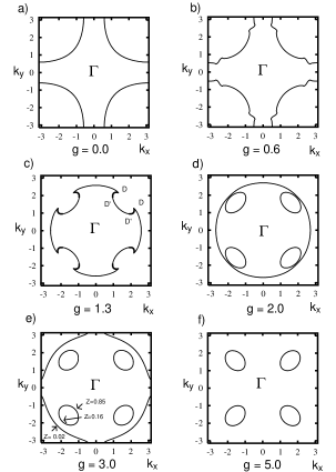
FIG. 13.: Fermi surface evolution with increasing $g$. We used (in units of $t$), $\Delta_{0}=0.1$, $\omega_{0}=0.3$, $t^{\prime}=-0.45$, $x=0.1$. For these parameters we obtain $g^{(1)}_{cr}=0.42$, and $g^{(2)}_{cr}\approx 1.64$. The figures are for $g=0$, $2\omega_{0}>g>g^{(1)}_{cr}$ , $g^{(2)}_{cr}>g>2\omega_{0}$, $g\geq g^{(2)}_{cr}$, $g>g^{(2)}_{cr}$, and $g\gg g^{(2)}_{cr}$, respectively. In (c), the nested pieces of the Fermi surface are shown in bold. In Fig. (e), we also presented the values of the quasiparticle residue along the Fermi surface. Notice that the definition of $g$ used in this paper differs by a factor of $2$ from the one in Ref.[60].

In the Matsubara formalism, which is more convenient for computations, the self-energy at $T=0$ is given by

$$\Sigma(k,\omega_{m}) = {g^{2}\over(2\pi)^{3}}\int d^{2}q\,d\Omega_{m}\chi(q,\Omega_{m})$$ (42)

$$\times\,G_{0}(k+q,\omega_{m}+\Omega_{m})$$

As we discussed above, we will use the phenomenological form of the susceptibility in Eq.(6) with a cutoff $\omega_{0}$ in both momentum and frequency. The location of the Fermi surface is obtained from

$$G^{-1}_{full}(k,\omega_{m}=0)=-\bar{\epsilon}_{k}-\Sigma(k,\omega_{m}=0)~{}=~{}0$$ (43)

It is instructive to consider first the case when the spin damping is absent, because then we can obtain a full analytical solution for $\Sigma$. Since the susceptibility is peaked at $Q$, we can expand the energy of the internal fermion as $\epsilon_{k+q}=\epsilon_{k+Q}+{\vec{v}}_{k+Q}({\vec{q}}-{\vec{Q}})$. Substituting this expansion into Eq.(42) and integrating over momentum and frequency, we obtain a rather complex function of the ratio $a_{k}=v_{k+Q}/c_{sw}$ which we present in the Appendix. The formula for $\Sigma(k,\omega_{m})$ simplifies considerably if $a_{k}=1$. Then we have

$$\Sigma(k,\omega_{m})=\frac{g^{2}}{4}~{}{1\over i\omega_{m}-\bar{\epsilon}_{k+Q}}$$ (44)

if $\bar{\epsilon}^{2}_{k+Q}+\omega_{m}^{2}>\omega_{0}^{2}$ and

$$\Sigma(k,\omega_{m})=\frac{g^{2}}{4}~{}{1\over i\omega_{m}-\bar{\epsilon}_{k+Q}}~{}\frac{\sqrt{\omega^{2}_{m}+\bar{\epsilon}^{2}_{k+Q}+\Delta_{0}^{2}}-\Delta_{0}}{\sqrt{\omega^{2}_{0}+\Delta_{0}^{2}}-\Delta_{0}}$$ (45)

if $\bar{\epsilon}^{2}_{k+Q}+\omega_{m}^{2}<\omega_{0}^{2}$. Here we introduced $\Delta_{0}=c_{sw}/\xi.$

We have checked numerically that the qualitative picture for the evolution of the Fermi surface does not depend substantially on the value of $a_{k}$. We will therefore discuss the Fermi surface evolution by restricting with the form of the self-energy given in Eqs.(44) and (45).

The self-energy in Eq.(44) is precisely what we need to recover the SDW solution which, we recall, yields a small Fermi surface centered at $(\pi/2,\pi/2)$. However, to obtain this small Fermi surface, Eq.(44) should be satisfied (at zero frequency) for all points in $k-$space, and, in particular, for the points along the magnetic Brillouin zone boundary. At $g=0$, the hot spots are at $\bar{\epsilon}_{k}=\bar{\epsilon}_{k+Q}=0$. Clearly, at small $g$, the location of the Fermi surface near the hot spots is obtained with the self-energy from Eq.(45). A simple experimentation shows that the location of the Fermi surface crossing does not change with small enough $g$, i.e., it still occurs at $\bar{\epsilon}_{k}=\bar{\epsilon}_{k+Q}=0$. However, as $g$ increases, there appear two new hot spots at $\bar{\epsilon}_{k}\not=0$. To see this, consider a point at the magnetic zone boundary right near a hot spot. Expanding Eq.(45) in $\bar{\epsilon}_{k+Q}$ and substituting the result into Eq.(43), we obtain

$$G^{-1}_{full}(k,0)=-\bar{\epsilon}_{k}~{}\left(1-\frac{g^{2}}{8\Delta_{0}\Big{(}\sqrt{\omega^{2}_{0}+\Delta_{0}^{2}}-\Delta_{0}\Big{)}}\right)$$ (46)

For sufficiently small $g$, the only solution for the Fermi surface is $\bar{\epsilon}_{k}=0$. However, when $g$ reaches the value $g_{cr}^{(1)}=2\omega_{0}[2\Delta_{0}/(\sqrt{\omega_{0}^{2}+\Delta_{0}^{2}}+\Delta_{0})]^{1/2}$, the velocity along the magnetic zone boundary vanishes. For larger $g$, one still has a Fermi-surface crossing at $\bar{\epsilon}_{k}=0$, however, two new hot spots appear (see Fig.13b) with

$$\bar{\epsilon}_{k}=\pm{g^{2}\over 4\Big{[}\sqrt{\omega_{0}^{2}+\Delta_{0}^{2}}-\Delta_{0}\Big{]}}\Bigg{(}1-{(g_{cr}^{(1)})^{2}\over g^{2}}\Bigg{)}^{1/2}$$ (47)

As $g$ increases, $|\bar{\epsilon}_{k+Q}|$ for the new hot spots also increases, and at $g=2\omega_{0}$, these new hot spots satisfy $|\epsilon_{k+Q}|=\omega_{0}$, i.e., they become the solutions of $G^{-1}_{full}(k,0)=0$ with the SDW-like form of the self-energy in Eq.(44) rather than the form in Eq.(45). These solutions have a very simple form: ${\bar{\epsilon}}_{k}=\pm g/2$. For even larger $g$, the SDW form of the solution for the Fermi surface extends beyond the hot spots and is located between points $D$ and $D^{\prime}$ in Fig.13c. As $g$ continues to increase, the $D$ and $D^{\prime}$ points from neighboring hot spots approach each other. Finally, at

$$g=g_{cr}^{(2)}=2\omega_{0}\Bigg{[}1+{8t(|\mu|-\omega_{0})\over\omega_{0}\Big{[}2t+\sqrt{4t^{2}-4|t^{\prime}|(|\mu|-\omega_{0})}\Big{]}}\Bigg{]}^{1/2}$$

these points merge and the system undergoes a topological, Lifshitz-type phase transition (Fig.13d) in which the singly-connected hole Fermi surface splits into hole pockets centered at $(\pm\pi/2,\pm\pi/2)$ and a large hole Fermi surface centered around $(\pi,\pi)$. As $g$ increases further, the large Fermi surface shrinks (Fig.13e) and eventually disappears at which point the Fermi surface just consists of four hole pockets (Fig.13f).

We found numerically that the topological phase transition at $g_{cr}^{(2)}$ is accompanied by drastic changes in the functional behavior of the system. To demonstrate this point we plot in Fig. 14a,b the chemical potential $\mu$ and the area of the electron states in the Brillouin zone as a function of $g$.

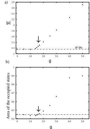
FIG. 14.: (a) The chemical potential as a function of the coupling, $g$. The parameters are the same as in Fig. 13. For free fermions, $\mu=\mu_{0}\approx-1.16$. The arrow indicates the value of $g^{(2)}_{cr}$ when hole pockets are formed. (b) The area of the occupied states vs $g$. The dashed line is the area for free fermions.

One clearly observes that both quantities are practically constant upto $g_{cr}^{(2)}$, but increase considerably for $g>g_{cr}^{(2)}$ (we attribute the small variations below $g_{cr}^{(2)}$ in Fig. 14b to numerical errors). In other words, Luttinger’s theorem is satisfied below $g_{cr}^{(2)}$, but is violated above this critical coupling. We attribute the violation of Luttinger’s theorem to the nonconvergence of the perturbative expansion in $g$ above $g_{cr}^{(2)}$. We remind in this regard that, in essence, Luttinger’s proof is perturbative: he showed that $I=\int G_{full}\partial\Sigma/\partial\omega=0$ order by order in perturbation theory. Implicit in this proof is the assumption that the perturbative series is convergent. We computed $I$ numerically and found that it is equal to zero (within the accuracy of our calculations) below $g_{cr}^{(2)}$ but rapidly increases as soon as $g$ exceeds the critical value. We reserve a detailed discussion of this issue for a separate publication.

Further, we mentioned in the introduction that it is still a subject of controversy whether the sides of the hole pockets which are facing $(\pi,\pi)$ have been observed in experiments or not. The relevant physical quantity here is the quasiparticle residue at the Fermi surface. For small $g$, when one has a large Fermi surface, $Z_{k}$ is almost $k-$independent and close to one. For very large $g$, when one effectively recovers the SDW form of the electronic excitations, $Z_{k}$ is again $k-$ independent and is equal to $1/2$. For intermediate $g$ , however, $Z_{k}$ is strongly $k-$dependent and anisotropic. The full expression for $Z_{k}$ is presented in the Appendix. The results for the case when hole pockets and a large Fermi surface coexist are presented (for $a_{k}=1$) in Fig.13e. We see that the quasiparticle residue along the large Fermi surface is very small, which makes the experimental observation practically impossible. Furthermore, we see that the quasiparticle residue of the side of the hole pocket which is facing $(\pi,\pi)$ is roughly five times smaller than the one in the momentum region facing the $\Gamma$ point. This may very well explain the experimental difficulties in observing the part of the hole pocket facing $(\pi,\pi)$.

Finally, we want to discuss how the above results change when we take a damping of spin fluctuations $\gamma=c^{2}_{sw}/(2\omega_{sf}\xi^{2})$ into consideration. We found that the general scenario of the Fermi surface evolution does not change, but that its onset occurs at substantially larger values of the coupling constant than in the absence of damping. Specifically, we found (still, assuming for simplicity that $a_{k}=1$) that the value of $g^{(1)}_{cr}$ where a hot spot splits into three is $g^{(1)}_{cr}(\gamma)=g^{(1)}_{cr}(\gamma=0)\Psi(\gamma/\Delta_{0})$ where $\Psi(x)=1-x/(3\pi)+O(x^{2})$ for $x\ll 1$, and $\Psi(x)=(16\log x/(\pi x))^{1/2}$ for $x\gg 1$. In the nearly antiferromagnetic Fermi liquid, $\gamma/\Delta_{0}=c_{sw}/(2\omega_{sf}\xi)$ is a large parameter. In this case, $g^{(1)}_{cr}\propto[\gamma/\log(\gamma/\Delta_{0})]^{1/2}$ which is substantially larger than $g^{(1)}_{cr}\propto(\Delta_{0})^{1/2}$ which we obtained in the absence of damping.

D Vertex corrections

The bare interaction vertex in the spin-fermion model is a momentum-independent constant $g$. At small couplings, the full vertex is indeed close to the bare one. At strong couplings, on the other hand, we have precursors of the SDW state, and, as we discussed, the full vertex should be much smaller than the bare one. We now study how the full vertex evolves with the coupling strength. Contrary to naive expectations, we find that the evolution of the vertex is not smooth. For definiteness, we will study below the vertex which describes the interaction between fermions at the hot spots and transverse spin fluctuations with antiferromagnetic momentum $Q$ and zero frequency. This vertex is relevant to the pairing problem since the incoming and outgoing fermions can simultaneously be placed on the Fermi surface.

Consider first the limit of weak coupling. The diagram for the vertex correction is presented in Fig. 8. Since the spin susceptibility is peaked at $Q$, the internal fermions are also located near the hot spots, and all three internal lines in the diagram carry low-energy excitations. A simple dimensional analysis shows that the vertex correction is logarithmically singular in the limit when the external fermionic frequencies are zero and the correlation length is large: $\Delta g\propto g*\log[max(\omega_{1,2},c_{sw}\xi^{-1})]$. In order to obtain an analytical expression for $\Delta g$, we expand the fermionic energies near the hot spots as $\epsilon_{k}=v_{h}(k-k_{h})\cos(\phi)$ and $\epsilon_{k+Q}=v_{h}(k-k_{h})\cos(\phi+\phi_{0})$ and perform the integration over frequency and momentum in the spin susceptibility. Keeping both, the logarithmically divergent and the $\xi$-independent terms in $\delta g$, we obtain for zero external fermionic frequency

$$\frac{\Delta g}{g} = -\frac{g^{2}Z^{2}\chi_{Q}\omega_{sf}}{\pi^{3}v_{h}^{2}}Re\Bigg{\{}\int_{0}^{\pi}~{}d\phi~{}\frac{\log[\sin(\phi/2)]}{\cos\phi+\cos\phi_{0}}$$ (49)

$$\quad\times\log\frac{\sin(\phi/2)}{\delta^{2}}\Bigg{\}}+O(\delta^{2})$$

where $\delta=c^{2}_{sw}/(2\gamma~{}v_{h}~{}\xi)\equiv\xi\omega_{sf}/v_{h}\ll 1$. $Z$ is the fermionic quasiparticle residue in the absence of the spin-fermion interaction and $\phi_{0}$ is the angle between the normals to the Fermi surface at $k$ and $k+Q$ (see Fig. 15).

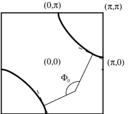
FIG. 15.: The graphical representation of the angle $\phi_{0}$ between the normals to the Fermi surface at hot spots (dashed lines). For clarification we omitted the parts of the Fermi surface in the second and fourth quadrant.

For the $t-t^{\prime}$ model for the quasiparticle dispersion we find $\phi_{0}=\pi/2+2tan^{-1}[(1-2|t^{\prime}|\sqrt{\mu/4t^{\prime}})/((1+2|t^{\prime}|\sqrt{\mu/4t^{\prime}})]$. Observe that $\Delta g$ does not depend on the upper cutoff in the frequency and momentum integration (i.e., on $\omega_{0}$).

We see that $\Delta g$ diverges logarithmically when $\xi$ diverges and $\delta\propto\xi^{-1}$ tends to zero. Alternatively, one can compute $\Delta g$ at $\xi^{-1}=0$ but at finite $\omega_{1,2}$, and also obtain a logarithmical divergence. This last result was also obtained by Altshuler et al.[15].

The integral in the right hand side of Eq.(49) can easily be evaluated numerically (and also analytically for particular values of $\phi_{0}$). It turns out that this integral is negative for all $\phi_{0}$, i.e., the relative vertex correction is positive. This implies that for small couplings, vertex corrections in fact increase the coupling strength and therefore enhance the $d-$wave pairing interaction. This is the opposite behavior of what we would expect at strong couplings. The strength of the vertex correction is another issue which recently was the subject of some controversy [15, 62, 63]. The key issue here is whether one should consider $\omega_{sf}$ as an independent input parameter, or assume that the damping is mainly due to the interaction with fermions. In the latter case, which we believe is closer to reality, $\omega^{-1}_{sf}$ by itself is proportional to $g^{2}Z^{2}/v_{h}^{2}$ in which case the coupling strength, fermionic velocity, and the bare quasiparticle residue are cancelled out in the r.h.s. of Eq.(49). In explicit form we found for $\omega_{sf}$

$$\omega_{sf}=\frac{\pi}{4}~{}|\sin\phi_{0}|~{}\frac{v_{h}^{2}}{g^{2}Z^{2}\chi_{Q}}.$$ (50)

Substituting $\omega_{sf}$ into Eq.(49) we obtain, neglecting terms of $O(\delta^{2})$

$$\frac{\Delta g}{g}=-\frac{|\sin\phi_{0}|}{4\pi^{2}}Re\int_{0}^{\pi}~{}d\phi~{}\frac{\log[\sin(\phi/2)]}{\cos\phi+\cos\phi_{0}}\log\frac{\sin(\phi/2)}{\delta^{2}}$$ (51)

This expression only depends on $\phi_{0}$. Numerically, the r.h.s. of Eq.(51) is small for all realistic values of $\delta$. Thus, for $\delta=0.27$, $t^{\prime}=-0.45t$, and $\mu=-1.16$ (which corresponds to 10% doping), we have $\Delta g/g\approx+0.04$. A similar result has been obtained in Ref.[15].

Notice that though the vertex correction is small numerically, Eq.(51) shows that the perturbative expansion for $\Delta g$ breaks down since $\Delta g$ exhibits a step-like behavior when $g$ becomes finite. This behavior of $\Delta g$, however, is just an artifact of our approximation in which we neglected the $\omega^{2}$ term compared to $\omega/\omega_{sf}$ in the spin susceptibility. A more detailed analysis shows that a continuous behavior of $\Delta g$ is restored for $g<\delta$.

Consider now what happens when $g$ increases and the Fermi surface starts to evolve. As we discussed in the previous subsection, the evolution begins at $g=g^{(1)}_{cr}$ with the flattening of the Fermi surface at the hot spots. For $g>g^{(1)}_{cr}$ there appear two satellites of the original hot spot (see Fig. 12b). The central hot spot is a solution of $\epsilon_{k}=\mu$ below and above $g^{(1)}_{cr}$, and the vertex corrections for this hot spot are virtually insensitive to the onset of the Fermi surface evolution (we recall that we restrict ourselves with the second-order correction which involves only bare fermionic propagators). On the other hand, for the two new hot spots, $\epsilon_{k}-\mu$ is finite (see Eq.(47)), and thus the vertex corrections will be different. As the Fermi surface continues to evolve, the old hot spot and one of the two new hot spots eventually disappear leaving a single new hot spot as the only remaining one on the Fermi surface. The vertex correction at this hot spot depends on the value of the chemical potential and changes sign when $|\mu|$, which grows with $g$ for $g>g^{(2)}_{cr}$, becomes comparable to the fermionic bandwidth. At even larger $g$, $|\mu|$ grows approximately as $g/2$. In this limit, the relative vertex correction becomes, to leading order in $\omega_{0}/g$, $\Delta g/g\approx-(g/\mu)^{2}\int d^{2}qd\Omega\chi_{aa}(q,\Omega)\approx-1$, i.e., the total vertex $g_{tot}=g+\Delta g$ is nearly zero. Performing calculations beyond the leading order in $\omega_{0}/g$ and for spin momentum $q\neq Q$, we found that in this limit,

$$g_{tot}(q)\propto\frac{\omega_{0}}{g}~{}~{}\left(\lambda^{2}\left(\frac{\omega_{0}}{g}\right)^{2}+(q-Q)^{2}\right)^{1/2},$$ (52)

where $\lambda=O(1)$ is a numerical factor. We see that for very large couplings, the vertex is nearly linear in $(q-Q)$ as it should be in the SDW phase.

The strong coupling form of the vertex is very similar to the one suggested by Schrieffer [46], the only difference is that in his expression, $(\omega_{0}/g)^{2}$ in Eq.(52) is replaced by $\xi^{-2}$. We argue that one needs more than just a large correlation length to recover the precursors of the SDW state in the electronic dispersion and the vertex. Namely, in our approach, the SDW form of the vertex appears due to a separation of the original fermionic dispersion into two subbands separated by an energy scale $g$ which is large compared to the cutoff $\omega_{0}$ in the spin susceptibility. When the correlation length becomes larger, $\omega_{0}$ clearly goes down (and hence, $g/\omega_{0}$ increases), but $\omega_{0}$ remains finite when $\xi$ becomes infinite. When the system becomes ordered, there appears a new momentum scale, $q_{0}\propto<S_{z}>$, such that when $|q-Q|<q_{0}$, $g_{tot}(q)$ is strictly linear in $|q-Q|$ in accordance with the Adler principle, while for larger momentum, one obtains a crossover to Eq.(52). For $q_{0}\gg(\omega_{0}/g)$, the difference between the two limits becomes negligible and one fully recovers the strong-coupling SDW result for the vertex.

IV Conclusions

We first summarize our results. The goal of this paper was to study the evolution of the electronic and magnetic properties of cuprates as one moves from optimal doping into the underdoped regime. Specifically, we were mostly interested in a possible relation between the reduction of $T_{c}$ with decreasing doping and the loss of the pieces of the Fermi surface near $(0,\pi)$ and related points, as evidenced in photoemission data. To address this issue, we considered an effective spin-fermion model in which itinerant fermions interact with low-energy spin fluctuations whose dynamics are described by a semi-phenomenological spin susceptibility which we assume to be peaked at the antiferromagnetic momentum. In the absence of the spin-fermion interaction, the fermions are assumed to form a Fermi liquid with a large Fermi surface which encloses an area roughly equal to half of the Brillouin zone. We argued that one can model the system’s evolution towards half-filling by increasing the strength of the spin-fermion interaction. The weak coupling limit models the situation near optimal doping, while the strong coupling limit corresponds to strongly underdoped cuprates. We found that, as the coupling increases, the Fermi surface first evolves in a continuous way, and its area remains unchanged. At some critical coupling, however, the system undergoes a topological, Lifshitz-type phase transition in which the singly connected hole Fermi surface centered at $(\pi,\pi)$ splits into a hole pocket centered at $(\pi/2,\pi/2)$, and a large hole Fermi surface centered at $(\pi,\pi)$. As $g$ increases further, the area of the large Fermi surface gradually decreases, and it eventually disappears. As a result, the Fermi surface at large enough $g$ consists of four small pockets. Simultaneously with the changes in the Fermi surface topology, the spin-fermion vertex also changes from being nearly constant at small $g$ to being nearly a linear function of $q-Q$ at strong couplings. This last form of the vertex is the one expected for an ordered antiferromagnet. When the vertex is linear in $q-Q$, one does not obtain an attractive interaction in the $d-$wave pairing channel since the enhancement of the spin susceptibility near $Q$ is fully compensated by the reduction of the vertex.

Our results, therefore, show that there is an interplay between the Fermi surface evolution and the loss of $d-$wave superconductivity in strongly underdoped cuprates. Both phenomena are related to the fact that the strong coupling SDW forms of the electronic dispersion and the spin-fermion vertex do not change drastically when the system looses long-range magnetic order, contrary to what one could expect from the mean-field theory. Instead, the electronic structure gradually changes towards a conventional Fermi liquid as magnetic correlations become less and less relevant. We believe that the Fermi liquid picture of electronic states, with one single peak in the density of states, is restored somewhere around optimal doping.

As we already mentioned in the introduction, the transformation from a large to a small Fermi surface in underdoped cuprates is consistent with the experimental data, though only one group so far reported the observation of both sides of the hole pocket. We emphasize, however, that in the intermediate coupling regime, which most probably corresponds to the experimental situation for $T_{c}=30K$ and $T_{c}=60K$ $Bi2212$ superconductors studied by photoemission [7, 8, 9], the quasiparticle residue for the part of the pocket which faces $(\pi,\pi)$ is rather small (few times smaller than on the other side of the pocket) which makes it more difficult to extract the quasiparticle peak from the background.

There are several issues which are not resolved in this paper and require further study. First, the photoemission data indicate that the quasiparticle peak in the spectral function is broad already at optimal doping and becomes even broader as the system moves towards half-filling. We have shown in Sec. II A that at exactly half-filling, the broadening of the quasiparticle dispersion is due to the interaction with short wavelength spin fluctuations (long wavelength fluctuations do not contribute because of the vanishing vertex). In our analysis of the spin-fermion model with a cutoff $\omega_{0}$ in the susceptibility, we completely neglected these fluctuations in the paramagnetic phase (we remind that in our discussion on the cancellation of the higher-order self-energy diagrams, we restricted with only the leading terms in the expansion in the bosonic frequency and the momentum shift from $Q$. We do not believe that the qualitative features of the Fermi-surface evolution will change if we include short-wavelength spin fluctuations, but they can be important for a quantitative analysis. For example, the FLEX calculations, which do not yield precursors of the SDW state, also show that $T_{c}$ is reduced in underdoped cuprates simply because fermions become less coherent as one approaches half-filing [64].

Another issue which requires further study has emerged from the photoemission data from the Stanford and Argonne groups [7, 9] which found that, in underdoped cuprates, $A(\omega)$ for $k$ near $(0,\pi)$ not only has a broad peak at about $2J$, as it should be if the precursors of the SDW state are present, but also drops rapidly at frequencies of about $30meV$. There is no such drop for the data taken along the Brillouin zone diagonal. When the temperature is lowered below $T_{c}$, the spectral function acquires a narrow peak at exactly the same position where the drop has been observed [65]. It is tempting to associate this new feature with the precursors of the $d-$wave pairing state. Emery and Kivelson proposed a scenario for $d-$wave precursors in which proximity to the antiferromagnetic instability is not particularly relevant [66]. A similar scenario has been suggested by Randeria et al. [67]. From our perspective, an important point is the observation by Shen et al. [31] that both, the high energy peak and the drop in $A(\omega)$ at low energies disappear at about the same doping concentration, i.e., the two features are likely to be correlated. This observation poses the question whether precursors of the SDW state can give rise to precursors of the $d-$wave pairing state. At the moment, we do not know the answer to this interesting question.

Finally, the reasons why Luttinger’s theorem does not work above the critical value of the coupling are still not completely clear to us. Recently, we considered in detail why Luttinger’s proof for $I=\int G_{full}\partial\Sigma/\partial\omega=0$ does not work in the magnetically-ordered state [68]. We found that though a formal application of Luttinger’s arguments yields $I=0$ to all orders in the SDW gap $\Delta$ in perturbation theory, the frequency integrals contain a hidden linear divergence and have to be regularized. When this regularization is done, one obtains that $I$ is finite, as it should be to recover Eq.(12), and for small $\Delta$ behaves as $I\propto\Delta^{2}$. We are currently studying whether the same reasoning can be applied above the topological transition in the paramagnetic phase.

We conclude with a final remark. In this paper, we studied the Fermi surface evolution as a function of the coupling strength at zero temperature. There exist, however, a number of experimental data which show temperature crossovers in various observables in the underdoped cuprates, most noticeably in the NMR relaxation rate, the uniform susceptibility and the resistivity. Recently, Pines, Stoikovich and one of us (A. Ch.) argued that these crossovers are related to the thermal evolution of the Fermi surface (or, more accurately, to the evolution of the quasiparticle peak in the spectral function) [69]. We refer the interested reader to Ref.[69] for a detailed discussion of this issue.

V acknowledgements

It is our pleasure to thank all colleagues with whom we discussed the issues considered in this paper. The research was supported by NSF DMR-9629839. A. Ch. is a Sloan fellow.

A The self-energy for arbitrary $a_{k}$

The explicit computation of Eq.(42) yields for arbitrary $a_{k}=|v_{k+Q}/c_{sw}|$

$$\Sigma(k,\omega_{m}) = -g^{2}_{eff}{\sqrt{(\bar{\epsilon}_{k+Q}-i\omega_{m})^{2}}\over\bar{\epsilon}_{k+Q}-i\omega_{m}}$$ (A2)

$$\times\;{1\over\Big{(}\sqrt{\omega_{0}^{2}+\Delta_{0}^{2}}-\Delta_{0}\Big{)}\sqrt{1-a_{k}^{2}}}\times A$$

where

$$\Delta_{0}=c_{sw}/\xi,\;g_{eff}^{2}=g^{2}\alpha{\sqrt{\omega_{0}^{2}+\Delta_{0}^{2}}-\Delta_{0}\over\pi}$$

and

$$A=\ln{{\sqrt{(\bar{\epsilon}_{k+Q}-i\omega_{m})^{2}+\omega_{0}^{2}(1-a_{k}^{2})}+\sqrt{(1-a_{k}^{2})(\omega_{0}^{2}+\Delta_{0}^{2})}\over\sqrt{(\bar{\epsilon}_{k+Q}-i\omega_{m})^{2}}+\Delta_{0}\sqrt{1-a_{k}^{2}}}}$$ (A3)

if $\bar{\epsilon}_{k+Q}+\omega_{m}^{2}f_{a}>a_{k}^{2}\omega_{0}^{2}$, and

$$A = \ln\Bigg{[}{\sqrt{(\bar{\epsilon}_{k+Q}-i\omega_{m})^{2}+\bar{\epsilon}_{k+Q}+\omega_{m}^{2}~{}f_{a}(1-a_{k}^{2})}\over a\Big{(}\sqrt{(\bar{\epsilon}_{k+Q}-i\omega_{m})^{2}}+\Delta_{0}\sqrt{1-a_{k}^{2}}\Big{)}}+$$ (A5)

$$+{\sqrt{(1-a_{k}^{2})(\bar{\epsilon}_{k+Q}+\omega_{m}^{2}~{}f_{a}+a_{k}^{2}\omega_{0}^{2})}\over a_{k}\Big{(}\sqrt{(\bar{\epsilon}_{k+Q}-i\omega_{m})^{2}}+\Delta_{0}\sqrt{1-a_{k}^{2}}\Big{)}}\Bigg{]}$$

if $\bar{\epsilon}_{k+Q}+\omega_{m}^{2}f_{a}>a_{k}^{2}\omega_{0}^{2}$ with

$$f_{a}={(1+a_{k})^{2}-3\over a_{k}}$$

For $a_{k}=1$ we recover the expressions presented in Eqs.(44) and (45).
We also can extract the quasiparticle residue at the Fermi surface. Substituting (A2) into

$${1\over Z_{k}}=1-{\partial\Sigma\over\partial\omega}\Bigg{|}_{\omega=\bar{\epsilon}_{k}}$$

we we obtain

$${1\over Z_{k}}=1+{g_{eff}^{2}\;B\over\Big{(}\sqrt{\omega_{0}^{2}+\Delta_{0}^{2}}-\Delta_{0}\Big{)}\Big{(}|\bar{\epsilon}_{k+Q}|+\Delta_{0}\sqrt{1-a_{k}^{2}}\Big{)}}$$ (A6)

where

$$B={\sqrt{\bar{\epsilon}_{k+Q}^{2}+\Delta_{0}^{2}a_{k}^{2}}-a_{k}^{2}\Delta_{0}+|\bar{\epsilon}_{k+Q}|\sqrt{1-a_{k}^{2}}\over|\bar{\epsilon}_{k+Q}|+\sqrt{1-a_{k}^{2}}\sqrt{\bar{\epsilon}_{k+Q}^{2}+\Delta_{0}^{2}a_{k}^{2}}}$$ (A7)

if $|\bar{\epsilon}_{k+Q}|<\omega_{0}a_{k}$ and

$$B = \Bigg{\{}\sqrt{\omega_{0}^{2}+\Delta_{)}^{2}}+{\omega_{0}^{2}\sqrt{1-a_{k}^{2}}-\Delta_{0}|\bar{\epsilon}_{k+Q}|\over\sqrt{\bar{\epsilon}_{k+Q}^{2}+\omega_{0}^{2}(1-a_{k}^{2})}}\Bigg{\}}$$ (A8)

$$\times {1\over\sqrt{1-a_{k}^{2}}\sqrt{\omega_{0}^{2}+\Delta_{0}^{2}}+\sqrt{\bar{\epsilon}_{k+Q}^{2}+\omega_{0}^{2}(1-a_{k}^{2})}}$$ (A9)

if $|\bar{\epsilon}_{k+Q}|>\omega_{0}a_{k}$. We plotted this result (for $a_{k}=1$) in Fig. 13e.

REFERENCES

- [1] J.G. Bednortz and K.A. Müller, Z. Phys. B 64, 189 (1986).
- [2] C.P. Slichter, in Strongly Correlated Electronic Systems, ed. by K.S. Bedell et al., (Addison Wesley, 1994).
- [3] V. Barzykin and D. Pines, Phys. Rev. B 52, 13585 (1995).
- [4] D. C. Johnson, Phys. Rev. Lett 32, 957 (1989).
- [5] N.P. Ong in Physical Properties of High Temperature Superconductors, ed. by D.M. Ginsberg (World Scientific, Singapore, 1990), Vol. 2.
- [6] Y. Iye in Physical Properties of High Temperature Superconductors, ed. by D.M. Ginsberg (World Scientific, Singapore, 1990), Vol. 3.
- [7] D.S. Marshall et al., Phys. Rev. Lett 76, 4841 (1996) (1996);Science 273, 325 (1996).
- [8] S. LaRosa, I. Vobornik, H. Berger, G. Margaritondo, C. Kendziora, R. J.Kelley, J. Ma, and M. Onellion, preprint, (1996).
- [9] H. Ding et al., Nature 382, 51 (1996).
- [10] H.Y. Hwang et al. Phys. Rev. Lett. 72, 2636 (1994).
- [11] A.V. Puchkov, D.N. Basov, and T. Timusk, preprint cond-mat 9611083.
- [12] P.W. Anderson, Science 235, 1196 (1987).
- [13] S. Chakravarty and P.W. Anderson, Phys. Rev. Lett. 72, 859 (1994).
- [14] P.A. Lee and X.-G. Wen, Phys. Rev. Lett. 76, 503 (1996).
- [15] B.L. Altshuler, L.B. Ioffe, and A.J. Millis, Phys. Rev. B 52, 415 (1995).
- [16] C.M. Varma et al., preprint (1996).
- [17] D. Pines, in High Temperature Superconductivity and the C60 Family, ed. H.C. Ren, p. 1 (Gordon and Breach, 1995).
- [18] F. M. Hayden et al, Phys. Rev. Lett. 76, 1344 (1996).
- [19] N. Curro, R. Corey, and C.P. Slichter, preprint (1996).
- [20] G. Blumberg, R. Liu, M.V. Klein, W.C. Lee, D.M. Ginsberg, C. Gu, B.W. Veal, and B. Dabrowski, Phys. Rev. B 49, 13296 (1994).
- [21] J.R. Kirtley, C.C. Tsuei, J.Z. Sun, C.C. Cji, Lock See Yu-Jahnes, A. Gupta, M. Rapp, and M.B. Ketchen, Nature 373, 225 (1995).
- [22] R.C. Dynes, Physica C 235-240, 225 (1994).
- [23] J. Betouras and R. Joynt, Europhys. Lett. 31, 119 (1995).
- [24] C. Kendziora, R.J. Kelley, and M. Onellion, Phys. Rev. Lett. 77, 727 (1996).
- [25] J. Annett, N. Goldenfeld, and S. Renn, in Physical Properties of High Temperature Superconductors, edited by D.M. Ginsberg (World Scientific, Singapore, 1990).
- [26] P. Monthoux and D. Pines, Phys. Rev. B 47, 6069 (1993); Phys. Rev. B 50, 16015 (1994); Phys. Rev. B 49, 4261 (1994).
- [27] P. Monthoux and D.J. Scalapino, Phys. Rev. Lett. 72, 1874 (1994).
- [28] D.S. Dessau et al., Phys. Rev. Lett. 71, 2781 (1993).
- [29] Z.-X. Shen and J.R. Schrieffer, preprint (1996).
- [30] B.I. Shraiman and E.D. Siggia, Phys. Rev. Lett 61, 467 (1988).
- [31] Z.-X. Shen, private communication.
- [32] There are two nonequivalent positions in the unit cell of compounds which by itself can generate modulations.
- [33] P.W. Anderson and J.R. Schrieffer, Phys. Today 44, 55 (1991).
- [34] N. Bulut, D.J. Scalapino, and S.R. White, Phys. Rev. B 47, 2742 (1993).
- [35] A.P. Kampf , Phys. Rep. 249, 219 (1994).
- [36] F.C. Zhang and T.M. Rice, Phys. Rev. B 37, 3759 (1988); S.B. Bacci, R. Gagliano, R.M. Martin, and J.F. Annett, Phys. Rev. B 44, 11068 (1990).
- [37] D.J. Scalapino, Phys. Rep. 250, 329 (1995).
- [38] A. V. Chubukov and D. Frenkel, Phys. Rev. B 46, 11884 (1992).
- [39] S. Sachdev, A.V. Chubukov, and A. Sokol, Phys. Rev. B 51, 14874 (1995).
- [40] A. Millis, H. Monien, and D. Pines, Phys. Rev. B 42, 167 (1990).
- [41] A.V. Chubukov, P. Monthoux, and D.K. Morr, Phys. Rev. B (RC) submitted.
- [42] J.R. Schrieffer, X.G. Wen, and S.C. Zhang, Phys. Rev. B 39, 11663 (1989).
- [43] M. S. Hybertsen, E. B. Stechel, M. Schluter, and D. R. Jennison, Phys. Rev. B 41, 11068 (1990).
- [44] A.V. Chubukov and K.A. Musaelian, Phys. Rev. B 50, 6238 (1994).
- [45] D. Duffy and A. Moreo, Phys. Rev. B 52, 15607 (1995).
- [46] J.R. Schrieffer, J. Low Temp. Phys. 99, 397 (1995).
- [47] Indeed, very near , is linear in for any coupling. In the weak coupling limit, however, quickly saturates to its bare value.
- [48] I. Affleck and F.D.M Haldane, Phys. Rev. B 36, 5291 (1987).
- [49] D.K. Morr and A.V. Chubukov, in preparation.
- [50] C.L. Kane, P.A. Lee, and N. Read, Phys. Rev. B 39, 6880 (1989).
- [51] B.O. Wells et al, Phys. Rev. Lett. 74, 964 (1995).
- [52] S. LaRosa et al., preprint, cond-mat 9512132.
- [53] E. Dagotto, Rev. Mod. Phys. 66, 763 (1994).
- [54] R. Preuss, W. Hanke, and W. von der Linden, Phys. Rev. Lett. 75, 1344 (1995).
- [55] We do not consider here possible exponential tails in the density of states (Lifshitz tails).
- [56] That the isotropic dispersion near is the intrinsic property of the Hubbard model was first suggested by Laughlin: R.B. Laughlin, preprint cond-mat 9608005.
- [57] M. Rozenberg, G. Kotliar, H. Kaleuter, G.A. Thomas, D.H. Rapkine, J.M. Honig, and P. Metcalf, Phys. Rev. Lett. 75, 105 (1995).
- [58] A.P. Kampf and J.R. Schrieffer, Phys. Rev. B 42, 7967 (1990).
- [59] A.V. Chubukov, S. Sachdev, and T. Senthil, Nucl. Phys. B B426, 601 (1994).
- [60] A.V. Chubukov, D.K. Morr, and K.A. Shakhnovich, Phil. Mag. B 74, 563 (1996).
- [61] R. Hlubina and T.M. Rice, Phys. Rev. B 51, 9253 (1995); Phys. Rev. B 52, 13043 (1995).
- [62] A.V. Chubukov, Phys. Rev. B 52, R3840 (1995).
- [63] M.H. Sharifzadeh and P.C.E Stamp, Phys. Rev. Lett. 77, 301 (1996). Notice that their definition of is by a factor of larger than ours.
- [64] M. Langer, J. Schmalian, S. Grabowski, and K.-H. Bennemann, Phys. Rev. Lett. 75, 4508 (1995).
- [65] By itself, this result, if interpreted in the framework of the conventional BCS theory, implies that the density of particles which contribute to the coherent peak at the superconducting gap is much smaller than the total density of fermions.
- [66] V.J. Emery and S.A. Kivelson, Phys. Rev. Lett. 74, 3253 (1995).
- [67] M. Randeria, N. Trivedi, A. Moreo, and R.T. Scalettar, Phys. Rev. Lett. 72, 3292 (1994).
- [68] A. V. Chubukov et al., in preparation.
- [69] A.V. Chubukov, D. Pines, and B.P. Stojkovic, J. Phys. Condens. Matter 8, 10017 (1996).