Crossover between Luttinger and Fermi liquid behavior in weakly coupled metallic chains

Abstract

We use higher-dimensional bosonization to study the normal state of electrons in weakly coupled metallic chains interacting with long-range Coulomb forces. Particular attention is paid to the crossover between Luttinger and Fermi liquid behavior as the interchain hopping $t_{\bot}$ is varied. Although in the physically interesting case of finite but small $t_{\bot}$ the quasi-particle residue does not vanish, the single-particle Green’s function exhibits the signature of Luttinger liquid behavior (i.e. anomalous scaling and spin-charge separation) in a large intermediate parameter regime. Using realistic parameters, we find that the scaling behavior in this regime is characterized by an anomalous dimension of the order of unity, as suggested by recent experiments on quasi-one-dimensional conductors. Our calculation gives also new insights into the approximations inherent in higher-dimensional bosonization; in particular, we show that the replacement of a curved Fermi surface by a finite number $M$ of flat patches can give rise to unphysical nesting singularities in the single-particle Green’s function, which disappear only in the limit $M\rightarrow\infty$ or if curvature effects are included. We also compare our approach with other methods. This work extents our recent letter [Phys. Rev. Lett. 74, 2997 (1995).].

I Introduction

The properties of the normal metallic state of correlated electrons in $d=1$ dimension are usually summarized under the name Luttinger liquid behavior [1]. The single-particle Green’s function of a Luttinger liquid exhibits several striking differences to the Green’s function of a conventional Fermi liquid: the absence of a coherent quasi-particle peak, spin-charge separation, and anomalous scaling properties characterized by interaction-dependent power laws. Non-Fermi liquid behavior has recently been observed in several experiments. First of all, the normal-state properties of the high-temperature superconductors cannot be interpreted in terms of a conventional Fermi liquid picture [2]. Motivated by this experimental fact, Anderson [3] proposed that even in $d=2$ the single-particle Green’s functions of correlated electrons can exhibit Luttinger liquid behavior. This unconventional normal-state behavior was then shown to be a possible key to understand the novel superconducting state. In fact, the interlayer-tunneling theory of high-temperature superconductivity advanced by Chakravarty, Anderson and co-workers [4] is based on the fundamental assumption that in the normal state the single-particle Green’s function $G({\bf{k}},\omega)$ satisfies for wave-vectors ${\bf{k}}$ sufficiently close to the Fermi surface and for sufficiently low frequencies $\omega$ (measured relative to the chemical potential) an anomalous scaling law of the form

$$G({\bf{k}}^{\alpha}+s{\bf{q}},s\omega)=s^{\gamma-1}G({\bf{k}}^{\alpha}+{\bf{q}},\omega)\;\;\;,$$ (1)

where ${\bf{k}}^{\alpha}$ is a wave-vector on the Fermi surface, and $\gamma>0$ is some interaction-dependent exponent, the anomalous dimension. A finite value of $\gamma$ is one of the fundamental characteristics of Luttinger liquid behavior, whereas in a Fermi liquid $\gamma=0$. It should be stressed, however, that a generally accepted microscopic derivation of Eq. (1) for interacting fermions in $d>1$ does not exist.

Another class of materials where non-Fermi liquid behavior appears to have been observed experimentally consists of weakly coupled metallic chains [5], which are based on highly anisotropic conductors. Although at sufficiently low temperatures $T$ these systems have the tendency to develop various types of long-range order, above the ordering temperature the metallic state displays clearly non-Fermi liquid behavior. The interpretation of recent photoemission studies of these systems in terms of the Luttinger liquid picture leads to values for the anomalous dimension $\gamma$ in the range $1.0\pm 0.2$ [6, 7, 8]. Because in one-dimensional lattice models with short-range interactions (such as the Hubbard model) the anomalous dimension is always small compared with unity [9], the large experimentally measured value of $\gamma$ suggests that the long-range nature of the Coulomb interaction must play an important role in these systems. Of course, the experimental systems are not strictly one-dimensional, because the interchain hopping $t_{\bot}$ is small but finite, and even for $t_{\bot}=0$ the electrons on different chains interact with three-dimensional Coulomb forces. We thus arrive at the problem of weakly coupled metallic chains, which is the central topic of this paper.

In the last years the problem of coupled Luttinger liquids has been studied by many authors [10, 11, 12, 13, 14, 15, 16, 17, 18, 19, 20, 21, 22, 23]. Given the fact that in the absence of interchain hopping the non-perturbative bosonization approach can be used to calculate the single-particle Green’s function in a controlled way, some authors [12, 13, 17, 20, 22, 23] have attempted to supplement the one-dimensional non-perturbative bosonization solution by some kind of perturbation theory in powers of $t_{\bot}$. One disadvantage of this strategy is that in this way interchain hopping and electron-electron interactions between the chains are not taken into account on equal footing. In this work we shall therefore adopt a different strategy: Instead of combining one-dimensional bosonization with perturbation theory in powers of $t_{\bot}$, we shall use the recently developed higher-dimensional generalization of the bosonization method [24, 25, 26, 27, 28, 29, 30] to treat interchain hopping and interactions between the chains on equal footing. Thus, our approach is non-perturbative in $t_{\bot}$ and in the interaction. In particular, for $t_{\bot}=0$ we recover the well-known one-dimensional bosonization result for the Green’s function of the Tomonaga-Luttinger model.

The rest of this paper is organized as follows: In Sec. II we briefly describe the higher-dimensional bosonization approach. In particular, we emphasize the approximations inherent in this approach and discuss its limitations. In Sec. III we shall show how the problem of electrons that are confined to one-dimensional chains (i.e. without interchain hopping) and interact with three-dimensional Coulomb forces can be solved in a straightforward way with higher-dimensional bosonization. Of course, this problem can also be solved by means of the conventional one-dimensional bosonization technique [31, 32, 33]. However, as shown in Sec. IV, our approach can also handle the case of finite interchain hopping $t_{\bot}$ without having to rely on an expansion in powers of $t_{\bot}$ or in the interaction. Although the quasi-particle residue is found to be finite for any $t_{\bot}\neq 0$, we show by explicit calculation that there exists a large intermediate regime where the equal time Green’s function satisfies an anomalous scaling relation similar to a Luttinger liquid. In Sec. V we compare our results with those obtained by other approaches. Finally, in Sec. VI we present our conclusions.

II Higher-dimensional bosonization

In this section we shall give a brief summary of the higher-dimensional bosonization approach. The foundations of this novel non-perturbative approach to the fermionic many-body problem go back to ideas due to Luther [24] and Haldane [25]. More recently, a number of authors have applied this technique to problems of physical interest [26, 27, 28, 29]. The basis of higher-dimensional bosonization is the subdivision of the Fermi surface into a finite number of patches $P^{\alpha}_{\Lambda}$, $\alpha=1,\ldots,M$. To be specific, let us consider in Fig. 1 a typical Fermi surface associated with a periodic array of chains coupled by weak interchain hopping. A possible subdivision into $M=8$ patches is shown in Fig. 2. Each patch $P^{\alpha}_{\Lambda}$ is then extended into a $3$-dimensional squat box [26] as shown in Fig. 3. The characteristic size $\Lambda$ of the patches should be chosen sufficiently small so that within a given patch the curvature of the Fermi surface can be locally ignored. On the other hand, the cutoffs $\Lambda$ and $\lambda$ cannot be taken arbitrarily small, because higher-dimensional bosonization becomes only useful in practice if it is possible to ignore momentum transfer between different patches (the so-called around-the-corner processes [28]). Of course, this is only possible if the interaction is dominated by forward scattering. More quantitatively, we assume that the two-body interaction $f_{\bf{q}}$ becomes negligibly small if $|{\bf{q}}|$ is larger than some cutoff $q_{c}\ll\mbox{min}\{\Lambda,\lambda\}$. The geometry is shown in Fig. 3. Assuming that the nature of the interaction is such that the above condition can be satisfied, it is reasonable to make the following two approximations [28, 29]: First of all, we ignore momentum transfer between different boxes (diagonal-patch approximation). The relative number of matrix elements neglected in this case is in $d$ dimensions of order $q_{c}^{d}/(\Lambda^{d-1}\lambda)\ll 1$. The second fundamental approximation is the local linearization of the energy dispersion. Measuring wave-vectors locally with respect to coordinate systems located at points ${\bf{k}}^{\alpha}$ in the centers of the patches (see Fig. 3), a general energy dispersion $\epsilon_{\bf{k}}$ may be expanded as

$$\epsilon_{{\bf{k}}^{\alpha}+{\bf{q}}}=\epsilon_{\bf{k}^{\alpha}}+\xi^{\alpha}_{\bf{q}}\;\;\;,\;\;\;\xi^{\alpha}_{\bf{q}}={\bf{v}}^{\alpha}\cdot{\bf{q}}+\frac{(q_{\|}^{\alpha})^{2}}{2m^{\alpha}_{\|}}+\frac{(\bf{q}_{\bot}^{\alpha})^{2}}{2m^{\alpha}_{\bot}}+\ldots\;\;\;,$$ (2)

where $q_{\|}^{\alpha}={\bf{q}}\cdot\hat{\bf{v}}^{\alpha}$ and ${\bf{q}}_{\bot}^{\alpha}={\bf{q}}-({\bf{q}}\cdot\hat{\bf{v}}^{\alpha})\hat{\bf{v}}^{\alpha}$. Here $\hat{\bf{v}}^{\alpha}={\bf{v}}^{\alpha}/|{\bf{v}}^{\alpha}|$ is a unit vector in the direction of ${\bf{v}}^{\alpha}$. Note that in general the masses $m^{\alpha}_{\|}$ and $m^{\alpha}_{\bot}$ depend on the patch-index. Because in the grand-canonical formulation of statistical mechanics the energy dispersion appears only in the combination $\epsilon_{\bf{k}}-\mu$, the chemical potential $\mu$ cancels the constant $\epsilon_{\bf{k}^{\alpha}}$ in Eq. (2) provided ${\bf{k}}^{\alpha}$ is chosen to lie exactly on the Fermi surface. We now ignore all terms in Eq. (2) that are quadratic and higher order in ${\bf{q}}$, i.e. we approximate $\xi^{\alpha}_{\bf{q}}\approx{\bf{v}}^{\alpha}\cdot{\bf{q}}$. In particular, the term $({\bf{q}}^{\alpha}_{\bot})^{2}/(2m_{\bot}^{\alpha})$ is neglected. Note that retaining this term would lead to patches with non-zero curvature. Once we accept the validity of the above approximations, the single-particle Green’s function can be calculated without further approximation in arbitrary dimension. As shown in Refs. [28] and [29], the result for the Matsubara Green’s function at finite inverse temperature $\beta$ can be written as

$$G({\bf{k}}^{\alpha}+{\bf{q}},i\tilde{\omega}_{n})=\int d{\bf{r}}\int_{0}^{\beta}d\tau e^{-i({\bf{q}}\cdot{\bf{r}}-\tilde{\omega}_{n}\tau)}G^{\alpha}_{0}({\bf{r}},\tau)e^{Q^{\alpha}({\bf{r}},\tau)}\;\;\;,$$ (3)

where

$${{G}}^{\alpha}_{0}({\bf{r}},\tau)=\frac{1}{\beta V}\sum_{{\bf{q}},\tilde{\omega}_{n}}\frac{e^{i({\bf{q}}\cdot{\bf{r}}-\tilde{\omega}_{n}\tau)}}{i\tilde{\omega}_{n}-{\bf{v}}^{\alpha}\cdot{\bf{q}}}\;\;\;,$$ (4)

and the Debye-Waller factor $Q^{\alpha}({\bf{r}},\tau)$ is given by

$$Q^{\alpha}({\bf{r}},\tau)=R^{\alpha}-S^{\alpha}({\bf{r}},\tau)\;\;\;,$$ (5)

with

$$R^{\alpha} = \frac{1}{\beta{{V}}}\sum_{{\bf{q}},\omega_{m}}\frac{f^{{RPA}}({\bf{q}},i\omega_{m})}{(i\omega_{m}-{\bf{v}}^{\alpha}\cdot{\bf{q}})^{2}}=S^{\alpha}(0,0)\;\;\;,$$ (6)

$$S^{\alpha}({\bf{r}},\tau) = \frac{1}{\beta{{V}}}\sum_{{\bf{q}},\omega_{m}}\frac{f^{{{RPA}}}({\bf{q}},i\omega_{m})\cos({\bf{q}}\cdot{\bf{r}}-{\omega}_{m}\tau)}{(i\omega_{m}-{\bf{v}}^{\alpha}\cdot{\bf{q}})^{2}}\;\;\;.$$ (7)

Here $\tilde{\omega}_{n}=2\pi(n+\frac{1}{2})/\beta$ are fermionic Matsubara frequencies, and $\omega_{m}=2\pi m/\beta$ are bosonic ones. $f^{{{RPA}}}({\bf{q}},i\omega_{m})$ is the screened interaction in random-phase approximation (RPA), which is given in terms of the bare interaction $f_{\bf{q}}$ and the non-interacting polarization $\Pi_{0}({\bf{q}},i\omega_{m})$ via the usual relation

$$f^{{{RPA}}}({\bf{q}},i\omega_{m})=\frac{f_{\bf{q}}}{1+f_{\bf{q}}\Pi_{0}({\bf{q}},i\omega_{m})}\;\;\;.$$ (8)

In the RPA screened interaction Eq. (8) only the long wavelength limit of $\Pi_{0}({\bf q},i\omega_{m})$ enters, consistent with the neglect of the around-the-corner processes. Thus, the ${\bf{q}}$ sums in Eqs. (4)–(7) are implicitly restricted to the regime $|q_{\|}|{\raisebox{-2.15277pt}{$\;\stackrel{{\scriptstyle<}}{{\sim}}\;$}}\lambda$, $|q_{\bot}|{\raisebox{-2.15277pt}{$\;\stackrel{{\scriptstyle<}}{{\sim}}\;$}}\Lambda$. However, as long as the external wave-vector ${\bf{q}}$ in Eq. (3) is sufficiently small, we may ignore these cutoffs. Then it is easy to see that ${{G}}^{\alpha}_{0}({\bf{r}},\tau)$ in Eq. (4) is proportional to $\delta^{(d-1)}({\bf{r}}_{\bot})$, where the $d-1$-dimensional vector ${\bf{r}}_{\bot}$ consists of the components of ${\bf{r}}$ that are perpendicular to ${\bf{v}}^{\alpha}$. In fact, for $V$ and $\beta\rightarrow\infty$ the integration in Eq. (4) is easily performed analytically, with the result

$$G^{\alpha}_{0}({\bf{r}},\tau)=\delta^{(d-1)}({\bf{r}}_{\bot})\left(\frac{-i}{2\pi}\right)\frac{1}{r_{\|}+i|{\bf{v}}^{\alpha}|\tau}\;\;\;,$$ (9)

where $r_{\|}={\bf{r}}\cdot\hat{\bf{v}}^{\alpha}$. Because of the prefactor $\delta^{(d-1)}({\bf{r}}_{\bot})$, we may replace ${\bf{r}}\rightarrow r_{\|}\hat{\bf{v}}^{\alpha}$ in Eqs. (7) and (5). Furthermore the ${\bf{r}}$-integral in Eq. (3) is effectively a one-dimensional one, because the integrations over the components of ${\bf{r}}$ perpendicular to ${\bf{v}}^{\alpha}$ can be done trivially due to the $\delta$-function in Eq. (9). Of course, this simplification is an artefact of the linearization. The modifications of the above results due to the non-linear terms in the energy dispersion have recently been calculated in Ref. [30]. Most importantly, for non-linear energy dispersion one should replace in Eqs. (6) and (7)

$$\frac{1}{(i\omega_{m}-{\bf{v}}^{\alpha}\cdot{\bf{q}})^{2}}\rightarrow\frac{1}{(i\omega_{m}-\xi^{\alpha}_{\bf{q}})(i\omega_{m}+\xi^{\alpha}_{-\bf{q}})}\;\;\;,$$ (10)

where $\xi^{\alpha}_{\bf{q}}$ is given in Eq. (2). Note that the non-linear terms remove the double pole in Eqs. (6) and (7). Moreover, non-linearities in the energy dispersion lead also to the replacement of the function $G_{0}^{\alpha}({\bf{r}},\tau)$ in Eq. (3) by an interaction-dependent Green’s function $G_{1}^{\alpha}({\bf{r}},\tau)$, which does not involve the singular prefactor $\delta^{(d-1)}({\bf{r}}_{\bot})$ given in Eq. (9). For an explicit expression of $G_{1}^{\alpha}({\bf{r}},\tau)$ see Refs. [29] and [30].

The above non-perturbative expression for the single-particle Green’s function are valid in arbitrary dimensions and for arbitrarily shaped Fermi surfaces. Furthermore, in $d=1$ these expressions correctly reduce to the well-known bosonization result of the Tomonaga-Luttinger model. We now apply the above results to study the problem of coupled Luttinger liquids.

III The Coulomb-interaction in chains without interchain hopping

Before discussing finite interchain hopping $t_{\bot}$, it is instructive to study first the case $t_{\bot}=0$, where the electrons are confined to the individual chains. Of course, electrons on different chains still interact with the three-dimensional Coulomb interaction, so that this is not a purely one-dimensional problem. The latter has been discussed in Ref. [32]. Thus, making the continuum approximation for motion parallel to the chains, the Fourier transform of the bare interaction is given by

$$f_{\bf{q}}=e^{2}a_{\bot}^{2}\int_{-\infty}^{\infty}dr_{x}{\sum_{\bf{r}_{\bot}}}^{\prime}\frac{e^{-i{\bf{q}}\cdot{\bf{r}}}}{\sqrt{r_{x}^{2}+{\bf{r}}_{\bot}^{2}}}\;\;\;,$$ (11)

where the ${\bf{r}}_{\bot}$-sum is over the two dimensional lattice of chains, with interchain lattice spacing $a_{\bot}$. The prime indicates that the ${\bf{r}}_{\bot}=0$ term must be properly regularized (see below). For $|{\bf{q}}|\ll a_{\bot}^{-1}$ Eq. (11) reduces to the familiar result $f_{\bf{q}}=4\pi e^{2}/{\bf{q}}^{2}$. Note that we do not replace by hand the long-range Coulomb interaction by an effective screened short-range interaction. The screening problem will be solved explicitly via our bosonization approach.

Because for $t_{\bot}=0$ the particle number is conserved on each chain, the problem can be solved by means of standard one-dimensional bosonization techniques [31, 32, 33]. However, the solution can also be obtained quite elegantly within the framework of higher-dimensional bosonization. In the absence of interchain hopping, the Fermi surface consists of two parallel planes, as shown in Fig. 4. These planes can be identified with the patches discussed in Sec. II. Let us label the right plane by $\alpha=+$, and the left one by $\alpha=-$. The (linearized) energy dispersion is simply given by $\xi^{\alpha}_{\bf{q}}=\alpha v_{F}q_{x}$, where $v_{F}=|{\bf{v}}^{\alpha}|$ is the Fermi velocity. As usual, a dimensionless measure for the strength of the interaction is $F_{\bf{q}}=\nu f_{\bf{q}}$, where $\nu={2}/({\pi v_{F}a_{\bot}^{2}})$ is the density of states at the Fermi energy (the factor of $2$ is due to the spin-degeneracy). An important length scale in the problem is set by the Thomas-Fermi screening wave-vector $\kappa$, which can be defined by rewriting the dimensionless interaction $F_{\bf{q}}$ in the long wavelength limit as $F_{\bf{q}}=\kappa^{2}/{\bf{q}}^{2}$. This yields $\kappa=a_{\bot}^{-1}\sqrt{8\pi g}$, where the dimensionless coupling constant $g$ is given by

$$g=\frac{e^{2}}{\pi v_{F}}\;\;\;.$$ (12)

To evaluate Eqs. (5)–(7), we need to know the RPA interaction in Eq. (8), which involves the non-interacting polarization $\Pi_{0}({\bf{q}},i\omega_{m})$. In the absence of interchain hopping the polarization has the usual one-dimensional form, which is in the long wavelength limit given by

$$\Pi_{0}({\bf{q}},i\omega_{m})=\frac{\nu}{2}\sum_{\alpha=\pm}\frac{{\bf{v}}^{\alpha}\cdot{\bf{q}}}{{\bf{v}}^{\alpha}\cdot{\bf{q}}-i\omega_{m}}=\frac{\nu}{1+\omega_{m}^{2}/(v_{F}q_{x})^{2}}\;\;\;.$$ (13)

For better comparison with the calculations for finite interchain hopping presented in Sec. IV, it is convenient to express the RPA interaction in terms of the dynamic structure factor in the usual way (we take the limit $\beta\rightarrow\infty$)

$$f^{RPA}({\bf{q}},i\omega_{m})=f_{\bf{q}}-f_{\bf{q}}^{2}\int_{0}^{\infty}d\omega S^{RPA}({\bf{q}},\omega)\frac{2\omega}{\omega^{2}+\omega_{m}^{2}}\;\;\;,$$ (14)

with

$$S^{RPA}({\bf{q}},\omega)=\frac{1}{\pi}\mbox{Im}\left\{\frac{\Pi_{0}({\bf{q}},\omega+i0^{+})}{1+f_{\bf{q}}\Pi_{0}({\bf{q}},\omega+i0^{+})}\right\}\;\;\;.$$ (15)

Using Eq. (13) we obtain for $\omega>0$

$$S^{RPA}({\bf{q}},\omega)=Z_{\bf{q}}\delta(\omega-\omega_{\bf{q}})\;\;\;,$$ (16)

with the collective mode and the residue given by

$$\omega_{{\bf{q}}} = \sqrt{1+F_{\bf{q}}}v_{F}|q_{x}|\;\;\;,$$ (17)

$$Z_{\bf{q}} = =\frac{\nu v_{F}|q_{x}|}{2\sqrt{1+F_{\bf{q}}}}=\frac{|q_{x}|}{\pi a_{\bot}^{2}\sqrt{1+F_{\bf{q}}}}\;\;\;.$$ (18)

Substituting these results into Eq. (6) it is then easy to show that

$$R^{\alpha}=-\frac{1}{V}\sum_{\bf{q}}f_{\bf{q}}^{2}\frac{Z_{\bf{q}}}{(\omega_{\bf{q}}+|{\bf{v}}^{\alpha}\cdot{\bf{q}}|)^{2}}\;\;\;,$$ (19)

which for $V\rightarrow\infty$ reduces to

$$R^{\alpha}=-\frac{1}{2}\int_{0}^{\infty}\frac{dq_{x}}{q_{x}}\left<\frac{F_{\bf{q}}^{2}}{2\sqrt{1+F_{\bf{q}}}\left[\sqrt{1+F_{\bf{q}}}+1\right]^{2}}\right>_{BZ}\;\;\;.$$ (20)

Similarly, we obtain

$${\rm Re}S^{\alpha}(x,\tau) = -\frac{1}{2}\int_{0}^{\infty}\frac{dq_{x}}{q_{x}}\cos(q_{x}x)\left[\left<\frac{1+\frac{F_{\bf{q}}}{2}}{\sqrt{1+F_{\bf{q}}}}e^{-\sqrt{1+F_{\bf{q}}}v_{F}q_{x}|\tau|}\right>_{BZ}-e^{-v_{F}q_{x}|\tau|}\right]\;,$$ (21)

$${\rm Im}S^{\alpha}(x,\tau) = -\frac{\mbox{sgn}(\tau)}{2}\int_{0}^{\infty}\frac{dq_{x}}{q_{x}}\sin(q_{x}x)\left[\left<e^{-\sqrt{1+F_{\bf{q}}}v_{F}q_{x}|\tau|}\right>_{BZ}-e^{-v_{F}q_{x}|\tau|}\right]\;\;,$$ (23)

where $x=\alpha r_{x}$, and where for any function $h({\bf{q}})$ the symbol $\left<h({\bf{q}})\right>_{BZ}$ denotes averaging over the first transverse Brillouin zone (BZ),

$$\left<h({\bf{q}})\right>_{BZ}=\frac{1}{(\frac{2\pi}{a_{\bot}})^{2}}\int_{-\frac{\pi}{a_{\bot}}}^{\frac{\pi}{a_{\bot}}}dq_{y}\int_{-\frac{\pi}{a_{\bot}}}^{\frac{\pi}{a_{\bot}}}dq_{z}h({\bf{q}})\;\;\;.$$ (25)

To show that the $q_{x}$-integrals in Eqs. (LABEL:eq:ReS3patch) and (LABEL:eq:ImS3patch) exist at large $q_{x}$ without the addition of an ultraviolet cutoff it is necessary to know the behavior of $F_{\bf q}$ for large $|{\bf q}|$. Trivially in the approximation $F_{\bf q}=\kappa^{2}/{\bf q}^{2}$ the interaction falls off as $|{\bf q}|^{-2}$. If one takes into account that the one-dimensional continuous and two-dimensional discrete Fourier transform (11) of the potential shows the same behavior (see below) it is easy to show from Eqs. (LABEL:eq:ReS3patch) and (LABEL:eq:ImS3patch) that after the BZ averaging the integrands for $\tau=0$ fall off like $(\kappa/|q_{x}|)^{5}$. Because the $q_{x}$-integrals exist, $\kappa$ plays the role of an ultraviolet cutoff. For finite $\tau$ the integrands in Eqs. (LABEL:eq:ReS3patch) and (LABEL:eq:ImS3patch) only fall off like $(\kappa/q_{x})^{2}$ but the $q_{x}$-integrals still exists.

Let us first consider the case $\tau=0$. Then we need to calculate the following Brillouin zone average

$$\gamma_{cb}({q_{x}})=\frac{1}{2}\left<\frac{F_{\bf{q}}^{2}}{2\sqrt{1+F_{\bf{q}}}[\sqrt{1+F_{\bf{q}}}+1]^{2}}\right>_{BZ}=\frac{1}{2}\left[\left<\frac{1+\frac{F_{\bf{q}}}{2}}{\sqrt{1+F_{\bf{q}}}}\right>_{BZ}-1\right]\;\;\;.$$ (26)

In the regime $g\ll 1$ the Thomas-Fermi screening length $\kappa^{-1}$ is large compared with the transverse lattice spacing $a_{\bot}$. Because in this case all wave-vector integrals are dominated by the regime $|{\bf{q}}|{\raisebox{-2.15277pt}{$\;\stackrel{{\scriptstyle<}}{{\sim}}\;$}}\kappa$ it is allowed to use the continuum approximation $f_{\bf q}=4\pi e^{2}/{\bf{q}}^{2}$ for the Fourier transform of the Coulomb potential. The averaging over the transverse Brillouin zone in Eq. (26) can then be done analytically, with the result

$$\gamma_{cb}({q_{x}})=\frac{e^{2}}{2\pi v_{F}}\frac{1}{\left[|q_{x}|/\kappa+\sqrt{1+(q_{x}/\kappa)^{2}}\right]^{2}}\;\;\;.$$ (27)

Hence,

$$Q^{\alpha}(x,0)=-\frac{e^{2}}{2\pi v_{F}}\int_{0}^{\infty}dq_{x}\frac{1-\cos(q_{x}x)}{\left[|q_{x}|/\kappa+\sqrt{1+(q_{x}/\kappa)^{2}}\right]^{2}}\;\;\;.$$ (28)

For $x\gg\kappa^{-1}$ it is now easy to show that

$$Q^{\alpha}(x,0)\sim-\gamma_{cb}\ln[\kappa x]\;\;\;,$$ (29)

with the anomalous dimension given by

$$\gamma_{cb}\equiv\lim_{q_{x}\rightarrow 0}\gamma_{cb}(q_{x})=\frac{e^{2}}{2\pi v_{F}}\;\;\;.$$ (30)

The logarithmic growth of the static Debye-Waller factor is one of the characteristics of a Luttinger liquid. Note that in a strictly one-dimensional model the long-range Coulomb interaction leads to a Wigner crystal phase [34] and not to a Luttinger liquid. In this case the anomalous dimension diverges in the thermodynamic limit. However, the Coulomb interaction between electrons on different chains removes this divergence, and leads to a Luttinger liquid[32] with modified spectral properties for $k\neq k_{F}$ (see below).

We would like to point out that Eq. (30) is only valid for $g\ll 1$, where $\gamma_{cb}\ll 1$. It would be incorrect to extrapolate this result to the regime where $g$ is of the order of unity, which is experimentally relevant. In order to calculate the anomalous dimension in this regime, the Fourier transform $f_{\bf{q}}$ of the interaction has to be properly calculated. For larger $g$ we have to take in to account the lattice structure in the transverse direction. To calculate the one-dimensional continuous and two-dimensional discrete Fourier transform (11) of the Coulomb potential it is necessary to regularize the ${\bf r}_{\perp}=0$-contribution as in the strictly one-dimensional case [34]. The characteristic feature of the regularized ${\bf r}_{\perp}=0$-term is its logarithmic divergence $-c\ln{(a_{0}q_{x})}$ for small $q_{x}$, where $a_{0}$ is the typical extension of the one-particle wave-function in the transverse direction and $c$ is a constant. The prefactor and the behavior at larger momenta depend on the special regularization procedure chosen. This divergence is responsible for the divergence of the anomalous dimension in the strictly one-dimensional model with Coulomb interaction, which leads to the Wigner crystal phase [34] of the one-dimensional electron gas. For $g\ll 1$ we already saw that the chains coupled by the three-dimensional Coulomb interaction are not in the Wigner crystal but in the Luttinger liquid phase. In the following we show that for arbitrary $g$ the term $-c\ln{(a_{0}q_{x})}$ for an infinite number of chains is exactly cancelled by a term $c\ln{(a_{\perp}q_{x})}$ from the ${\bf r}_{\perp}\neq 0$ part of the Fourier transform (11). Therefore the system is a Luttinger liquid for all $g$.

In our regularization procedure we assume that the one-particle wave function in the transverse direction is given by a Gaussian distribution corresponding to a harmonic confinement potential. We replace the ${\bf r}_{\perp}=0$-component in Eq. (11) by

$$\frac{a_{\perp}^{2}e^{2}}{a_{0}^{2}\pi}\int_{-\infty}^{\infty}d{\bf r}_{\perp}\int_{-\infty}^{\infty}dr_{x}\frac{e^{-iq_{x}r_{x}}e^{-{\bf r}_{\perp}^{2}/a_{0}^{2}}}{\left(r_{x}^{2}+{\bf r}_{\perp}^{2}\right)^{1/2}}$$ (31)

$$=\frac{a_{\perp}^{2}e^{2}}{a_{0}^{2}\pi}\int_{-\infty}^{\infty}d{\bf r}_{\perp}K_{0}(|{\bf r}_{\perp}|q_{x})e^{-{\bf r}_{\perp}^{2}/a_{0}^{2}},$$ (32)

where $K_{0}(x)$ denotes the modified Bessel function. The logarithmic divergence of $K_{0}$ for $x\to 0$ leads to the logarithmic behavior for small $q_{x}$ discussed above.

To obtain a fast convergence of the Fourier transform (11) for ${\bf r}_{\perp}\neq 0$, we use the Ewald summation technique [35]. With the help of the Theta function transformation

$$\sum_{{\bf r}_{\perp}}e^{-\alpha|{\bf r}_{\perp}|^{2}-i{\bf q}_{\perp}\cdot{\bf r}_{\perp}}=\frac{\pi}{a_{\perp}^{2}\alpha^{2}}\sum_{{\bf G}_{\perp}}e^{-|{\bf q}_{\perp}-{\bf G}_{\perp}|^{2}/(4\alpha)},$$ (33)

where ${\bf G}_{\perp}$ denotes a vector of the reciprocal lattice in the transverse direction and the integral

$$\frac{2}{\sqrt{\pi}}\int_{0}^{\infty}d\alpha e^{-(r_{x}^{2}+|{\bf r}_{\perp}|^{2})\alpha^{2}}=\frac{1}{\sqrt{r_{x}^{2}+|{\bf r}_{\perp}|^{2}}}\;\;\;,$$ (34)

one obtains

$$f_{\bf q} = 4\pi e^{2}\sum_{{\bf G}_{\perp}}\frac{\exp{\left\{-\left[q_{x}^{2}+|{\bf q}_{\perp}-{\bf G}_{\perp}|^{2}\right]/(4\alpha_{0})\right\}}}{q_{x}^{2}+|{\bf q}_{\perp}-{\bf G}_{\perp}|^{2}}$$ (38)

$$+2a_{\perp}^{2}e^{2}\int_{\alpha_{0}}^{\infty}\frac{d\alpha}{\alpha}\sum_{{\bf r}_{\perp}\neq 0}e^{-\alpha|{\bf r}_{\perp}|^{2}-i{\bf q}_{\perp}\cdot{\bf r}_{\perp}}$$

$$-2a_{\perp}^{2}a_{0}^{2}e^{2}\int_{0}^{\alpha_{0}}d\alpha\alpha\frac{1}{1+a_{0}^{2}\alpha^{2}}e^{-q_{x}^{2}/(4\alpha^{2})}$$

$$+2a_{\perp}^{2}e^{2}\int_{\alpha_{0}}^{\infty}\frac{d\alpha}{\alpha}\frac{1}{1+a_{0}^{2}\alpha^{2}}e^{-q_{x}^{2}/(4\alpha^{2})}.$$

For $\alpha\in[0,\alpha_{0}]$ we used in Eq. (34) the transformation Eq. (33) from the direct to the reciprocal lattice. Now $\alpha_{0}$ can be chosen in such a way that in the sums in the first and second line of Eq. (38) only a few lattice vectors contribute. In the following we always choose $\alpha_{0}=4/a_{0}$. For this $\alpha_{0}$ the sum in the second line in Eq. (38) can be completely neglected and in the first line only the vectors ${\bf G}_{\perp}=(m_{y}2\pi/a_{\perp},m_{z}2\pi/a_{\perp})$ with $m_{y}$ and $m_{z}\in[-5,5]$ contribute. The last two terms in Eq. (38) contain the ${\bf r}_{\perp}=0$-term of Eq. (11). From Eq. (38) it is easy to see that only for $|{\bf q}|\ll a_{\perp}^{-1}$ is is allowed to approximate the Fourier transform of the Coulomb potential by its continuum limit $4\pi e^{2}/{\bf q}^{2}$.

To determine the anomalous dimension from Eqs. (26) and (30), we have to take the $q_{x}\to 0$ limit in Eq. (38). For $q_{x}=0$ we obtain

$$\tilde{v}(q_{x}=0,{\bf q}_{\perp}) = 4\pi e^{2}\sum_{{\bf G}_{\perp}}\frac{\exp{\left\{-|{\bf q}_{\perp}-{\bf G}_{\perp}|^{2}/(4\alpha_{0})\right\}}}{|{\bf q}_{\perp}-{\bf G}_{\perp}|^{2}}$$ (41)

$$+2a_{\perp}^{2}e^{2}\int_{\alpha_{0}}^{\infty}\frac{d\alpha}{\alpha}\sum_{{\bf r}_{\perp}\neq 0}e^{-\alpha|{\bf r}_{\perp}|^{2}-i{\bf q}_{\perp}\cdot{\bf R}_{\perp}}$$

$$-2a_{\perp}^{2}e^{2}\ln{\left[4\frac{a_{0}}{a_{\perp}}\right]},$$

i.e. no logarithmic divergence. As already discussed above, the logarithmic divergence of the ${\bf r}_{\perp}=0$-term is exactly cancelled. Therefore the anomalous dimension is finite and can be calculated numerically following Eqs. (26) and (30). In the regularization procedure we introduced the new parameter $a_{0}$. Physically it is clear that only ratios $a_{\perp}/a_{0}>1$ are relevant for quasi-one-dimensional systems. In Fig. 7 we present numerical results for $\gamma_{cb}$ with $a_{\perp}/a_{0}=3$ (dotted line) and $a_{\perp}/a_{0}=6$ (dashed line). For comparison we also show $\gamma_{cb}$ using the continuum approximation $f_{\bf q}=4\pi e^{2}/{\bf q}^{2}$ (solid line). From Eq. (38) it is easy to show, that $F_{\bf q}$ falls off as $\kappa^{2}/{\bf q}^{2}$ for large $|{\bf q}|$. Therefore our above discussion concerning the existence of the integrals Eqs. (LABEL:eq:ReS3patch) and (LABEL:eq:ImS3patch) is also applicable to the lattice Fourier transform.

In a Luttinger liquid the momentum integrated spectral function $\rho(\omega)$, which apart from a one-electron dipole matrix element determines angular integrated photoemission, is algebraically suppressed near the chemical potential [36]

$$\rho(\omega)\propto|\omega|^{{\gamma}_{cb}}.$$ (42)

Recent photoemission studies of quasi-one-dimensional conductors suggest values for the anomalous dimension in the range $1.0\pm 0.2$ [6, 7, 8]. This would be hard to reconcile with a model involving short range interactions, as e.g. the anomalous dimension in the one-dimensional Hubbard model never exceeds $1/8$. A rough estimate of the dimensionless coupling $g$ for experimental relevant parameters following Ref. [5] leads to values of $g$ of the order of one. As seen from Fig. 7 our treatment using realistic Coulomb forces quite easily leads to anomalous dimensions in the experimental range.

In the following we discuss the momentum dependent spectral function $\rho^{<}(q_{x},\omega)$. In the strictly one-dimensional model with an interaction potential which is finite at $q=0$ it is known that for anomalous dimensions $\gamma$ smaller than $1/2$ a power law divergence occurs at the energy $v_{F}q$ and for $\gamma<1$ at $v_{c}q$, where $v_{c}$ is the long wavelength limit of the $q$-dependent charge excitation velocity (spin-charge separation) [37, 38]. From Eq. (17) one obtains for the coupled chains a ${\bf q}_{\perp}$-dependence of the charge velocity

$$v_{c}({\bf q}_{\perp})=\lim_{q_{x}\to 0}\frac{\omega_{\bf q}}{q_{x}}=v_{F}\sqrt{1+F_{{\bf q}_{\perp}}}.$$ (43)

It is not obvious from Eqs. (LABEL:eq:ReS3patch) and (LABEL:eq:ImS3patch) whether a charge peak occurs or not, because the charge-velocity $v_{c}({\bf q}_{\perp})$ is subject to the BZ averaging and the singularity can be washed out. On the other hand, because the spin velocity $v_{F}$ is independent of ${\bf{q}}_{\bot}$, one obtains for $\gamma_{cb}<\frac{1}{2}$ a sharp threshold singularity at $\omega=-v_{F}|q_{x}|$, just like in one dimension,

$$\rho_{+}^{<}(q_{x},\omega)\sim\Theta(v_{F}[q_{x}-k_{F}]-\omega)(v_{F}[q_{x}-k_{F}]-\omega)^{\gamma_{cb}-1/2}.$$ (44)

For $\gamma_{cb}>\frac{1}{2}$ the singularity is washed out, but the threshold survives. On the Fermi surface the BZ averaging is irrelevant and one obtains for $\gamma_{cb}<1$

$$\rho_{+}^{<}(k_{F},\omega)\sim\Theta(-\omega)(-\omega)^{\gamma_{cb}-1}$$ (45)

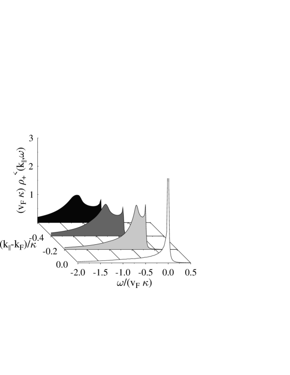
as in the one-dimensional Tomonaga-Luttinger model. In order to evaluate the momentum dependent spectral function for arbitrary $q_{x}$ and $\omega$, we have to use numerical techniques developed in Ref. [39]. It turns out that a broadened charge peak occurs. For increasing anomalous dimensions, i.e. increasing $g$, the charge peak broadens. To clearly demonstrate spin-charge separation, we present in Fig. 8 spectra for $\gamma_{cb}=0.33$, corresponding to $g=0.8$, with $a_{\perp}/a_{0}=3$. The spectra are calculated for large but finite systems. The system size is given by the dimensionless level spacing $\nu_{\kappa}=(2\pi/L)/\kappa$. In Fig. 8 we chose $\nu_{\kappa}=1/80$. For technical reasons we multiplied the Green’s function by a factor $\exp{\left\{-\chi|t|\right\}}$ before we performed the time-frequency Fourier transformation. This leads to a Lorentzian broadening of the discrete spectral function and smears out the threshold behavior at $\omega=v_{F}(k_{x}-k_{F})$. As can be seen from Fig. 8, the artificial broadening $\chi/(v_{F}\kappa)=0.01$ is much smaller than the natural broadening of the charge peak. The power law behavior of the spectra at $\omega=v_{F}(k_{x}-k_{F})$ leads to an asymmetry of the related peaks in Fig. 8. We checked that for a given $\chi$ the numerical spectra do not change if the system size is further increased. In the numerical calculations we have to cutoff the $q_{x}$-integrals in Eqs. (LABEL:eq:ReS3patch) and (LABEL:eq:ImS3patch) at $q_{x}=n\kappa$, with some number $n$. In Fig. 8 we chose $n=5$ but we checked that for the momenta and energies presented the spectra are the same for larger values of $n$. We found that the charge peak for $-0.5<(k_{x}-k_{F})/\kappa<0$ disperses like $\omega=\bar{v}_{c}(k_{x}-k_{F})$ with an effective $g$ dependent charge velocity $\bar{v}_{c}$ which has to be determined numerically. For anomalous dimensions larger than one no divergence at $\omega=v_{F}(k_{x}-k_{F})$ occurs and the spectra are dominated by a very broad charge peak.

To summarize this section, we showed that the system of one-dimensional chains coupled by the long ranged Coulomb interaction is a Luttinger liquid with an anomalous dimensions of the order of one. Furthermore the charge singularity of the strictly one-dimensional Luttinger liquid is broadened due to the BZ averaging, but is still present. In the following we extend the model and include transverse interchain hopping.

IV Finite interchain hopping

A typical Fermi surface of an array of chains with small finite interchain hopping is shown in Fig. 1. In the quasi-one-dimensional materials discussed in Ref. [5] the intrachain hopping $t_{x}$ is an order of magnitude larger than the interchain hopping $t_{y}=t_{\bot}$, which is again a factor of $10$ larger than $t_{z}$. We therefore assume transverse hopping only in the $y$ direction. In this section we shall apply our higher-dimensional bosonization approach to this problem. We would like to emphasize that we are ultimately interested in realistic Fermi surfaces without nesting symmetries. Unfortunately, by replacing a curved Fermi surface of the type shown in Fig. 1 by a finite number of locally flat patches (see Fig. 2), we introduce unphysical nesting symmetries. In order to obtain physical results that can be compared to experiments, the singularities caused by these artificial symmetries should therefore be separated from the physical plasmon mode in the dynamic structure factor. In this section we shall show how this can be done in practice.

A The $M$-patch model

In the higher-dimensional bosonization approach with linearized energy dispersion the Fermi surface is approximated by a finite number $M$ of flat patches $P^{\alpha}_{\Lambda}$. In order not to break the inversion symmetry of the Fermi surface, we choose an even number of patches of equal size such that for each $P^{\alpha}_{\Lambda}$ there exists another patch $P^{\bar{\alpha}}_{\Lambda}$ such that the local Fermi velocities satisfy ${\bf{v}}^{\bar{\alpha}}=-{\bf{v}}^{\alpha}$ (see Fig. 2 for $M=8$). Then the non-interacting polarization $\Pi_{0}({\bf{q}},z)$ is at long wavelengths given by

$$\Pi_{0}({\bf{q}},z)=\frac{2\nu}{M}\sum_{\alpha=1}^{M/2}\frac{({\bf{v}}^{\alpha}\cdot{\bf{q}})^{2}}{({\bf{v}}^{\alpha}\cdot{\bf{q}})^{2}-z^{2}}\;\;\;,$$ (46)

where it is understood that the sums are over all patches with ${\bf{v}}^{\alpha}\cdot{\bf{q}}\geq 0$. For finite $M$ the poles of the RPA interaction, which are simply the zeros of

$$1+f_{\bf{q}}\Pi_{0}({\bf{q}},z)=0\;\;\;,$$ (47)

can be easily obtained by plotting the right-hand side of Eq. (46) as function of $\omega^{2}$ where $\omega=z$ is real, and looking for the intersections with $-1/f_{\bf{q}}$. For generic ${\bf{q}}$ all $({\bf{v}}^{\alpha}\cdot{\bf{q}})^{2}$ are different and positive, and we can order $0<({\bf{v}}^{\alpha_{1}}\cdot{\bf{q}})^{2}<({\bf{v}}^{\alpha_{2}}\cdot{\bf{q}})^{2}<\ldots<({\bf{v}}^{\alpha_{M/2}}\cdot{\bf{q}})^{2}$. A repulsive interaction $f_{\bf{q}}$ leads then to zeros $(\omega_{\bf{q}}^{2})^{(\alpha)}$, $\alpha=1,\ldots,M/2$ of Eq. (47) as function of $z^{2}$ lying between the unperturbed poles,

$$({\bf{v}}^{\alpha_{1}}\cdot{\bf{q}})^{2}<(\omega_{\bf{q}}^{2})^{(1)}<({\bf{v}}^{\alpha_{2}}\cdot{\bf{q}})^{2}<\ldots<({\bf{v}}^{\alpha_{M/2}}\cdot{\bf{q}})^{2}<(\omega_{\bf{q}}^{2})^{(M/2)}\;\;\;.$$ (48)

In the large $M$-limit the first $M/2-1$ solutions form the particle-hole quasi-continuum, while the largest mode $\omega_{\bf{q}}^{M/2}$ can be identified with the collective plasmon mode. For ${\bf{q}}$-values which lead to ${\bf{v}}^{\alpha_{i}}\cdot{\bf{q}}=0$ and (or) $({\bf{v}}^{\alpha_{i}}\cdot{\bf{q}})^{2}=({\bf{v}}^{\alpha_{j}}\cdot{\bf{q}})^{2}$ the number of poles in the quasi-continuum with non-vanishing residue is reduced. Denoting by $Z_{\bf{q}}$ the residue of the plasmon mode, the dynamic structure factor is given by

$$S^{RPA}({\bf{q}},\omega)=Z_{\bf{q}}\delta(\omega-\omega_{\bf{q}})+S^{RPA}_{incoh}({\bf{q}},\omega)\;\;\;,$$ (49)

where $S^{RPA}_{incoh}({\bf{q}},\omega)$ is due to the contribution of the other modes, which merge for $M\rightarrow\infty$ into the particle-hole continuum. In the absence of interchain hopping $S^{RPA}_{incoh}({\bf{q}},\omega)=0$. Furthermore, the plasmon mode and the associated residue are given in Eqs. (17) and (18).

1 The plasmon mode

The crucial observation is now that for small but finite $t_{\bot}$ and $M\to\infty$ the low-energy behavior of the Green’s function is still dominated by the plasmon mode, which therefore describes the crossover between Luttinger and Fermi liquid behavior. Thus, to leading order in $\theta$, we may ignore the contribution $S^{RPA}_{incoh}({\bf{q}},\omega)$ in Eq. (49). In this case the constant part $R^{\alpha}$ of the Debye-Waller factor is still given by Eq. (19), but now with $\omega_{\bf{q}}$ and $Z_{\bf{q}}$ given by the plasmon mode of the $M$-patch model. In the strong coupling limit it is easy to obtain an analytic expression for $\omega_{\bf{q}}$ and $Z_{\bf{q}}$. Anticipating that at strong coupling there exists a pole $\omega_{\bf{q}}$ of Eq. (47) with $\omega_{\bf{q}}^{2}=O(F_{\bf{q}})$, we may expand $\Pi_{0}({\bf{q}},z)$ in powers of $z^{-2}$. The leading term is

$$\Pi_{0}({\bf{q}},z) = -\frac{2\nu}{M}\sum_{\alpha=1}^{M/2}\left(\frac{{\bf{v}}^{\alpha}\cdot{\bf{q}}}{z}\right)^{2}\left[1+\left(\frac{{\bf{v}}^{\alpha}\cdot{\bf{q}}}{z}\right)^{2}+O\left(\left[\frac{{\bf{v}}^{\alpha}\cdot{\bf{q}}}{z}\right]^{4}\right)\right]\;\;\;.$$ (50)

Substituting this approximation into Eq. (47), it is easy to show that

$$\omega_{\bf{q}}^{2} = F_{\bf{q}}\frac{2}{M}\sum_{\alpha=1}^{M/2}({\bf{v}}^{\alpha}\cdot{\bf{q}})^{2}+\frac{\sum_{\alpha=1}^{M/2}({\bf{v}}^{\alpha}\cdot{\bf{q}})^{4}}{\sum_{\alpha=1}^{M/2}({\bf{v}}^{\alpha}\cdot{\bf{q}})^{2}}+O\left(1/F_{\bf q}\right)$$ (51)

and

$$Z_{\bf{q}}=\frac{\nu}{2\sqrt{F}_{\bf{q}}}\left[\frac{2}{M}\sum_{\alpha=1}^{M/2}({\bf{v}}^{\alpha}\cdot{\bf{q}})^{2}\right]^{1/2}+O\left(1/F_{\bf q}\right)\;\;\;.$$ (52)

Introducing these expressions in Eq. (19) we obtain to leading order in the coupling

$$S_{pl}^{RPA}({\bf q},\omega)\approx\frac{\nu v_{F}}{2\sqrt{F_{\bf q}}}\sqrt{q_{x}^{2}+\eta^{2}{\bf q}_{\perp}^{2}}\delta\left(\omega-v_{F}\sqrt{F_{\bf q}}\sqrt{q_{x}^{2}+\eta^{2}{\bf q}_{\perp}^{2}}\right)\;\;,$$ (53)

where

$$\eta^{2}=\frac{2}{M}\sum_{\alpha=1}^{M/2}\left(\hat{\bf v}^{\alpha}\cdot\hat{\bf q}_{\perp}\right)^{2}$$ (54)

is a small parameter for a weakly corrugated Fermi surface corresponding to small interchain hopping. Note that ${\bf{q}}_{\bot}$ in Eq.(53) denotes the $q_{y}$- and $q_{z}$-components of ${\bf{q}}$, and should not be confused with the vector ${\bf{q}}^{\alpha}_{\bot}$ in Eq.(2). The contribution to the constant part $R_{pl}^{\alpha}$ of the Debye-Waller factor is given by

$$R^{\alpha}_{pl}=-\frac{1}{2}\int_{0}^{\infty}dq_{x}\left<\frac{1}{\sqrt{q_{x}^{2}+\eta^{2}q_{y}^{2}}}\frac{\sqrt{F_{\bf{q}}}}{\left[1+\frac{1}{\sqrt{F_{\bf q}}}\frac{{\bf{v}}^{\alpha}\cdot{\bf q}}{v_{F}\sqrt{q_{x}^{2}+\eta^{2}{\bf q}_{\perp}^{2}}}\right]^{2}}\right>_{BZ}\;\;\;.$$ (55)

To leading order the patch dependence drops out. For $\eta=0$, corresponding to zero interchain hopping the integral is logarithmically divergent. For finite $\eta$ the $q_{x}$ integration obtains a finite lower cutoff which leads to a contribution $\ln{[\kappa/(\eta|{\bf q}_{\perp}|)]}$. To leading order in $\ln{(1/\eta)}$ one can take the limit $q_{x}\rightarrow 0$ in $F_{\bf q}$. This yields

$$R^{\alpha}_{pl}\approx\frac{1}{2}\ln{(1/\eta)}\lim_{q_{x}\to 0}\left<\sqrt{F_{\bf q}}\right>_{BZ}\;\;\;.$$ (56)

The prefactor of the logarithm is just the strong coupling expression of the anomalous dimension of the zero hopping $\eta=0$ limit. Now, if $R_{pl}^{\alpha}$ is finite, the Riemann-Lebesgue Lemma [40] guarantees that $S_{pl}^{\alpha}(r_{\parallel}\hat{{\bf v}}_{\alpha},0)$ goes to zero for increasing $r_{\parallel}$. Therefore the system is no longer a Luttinger liquid, but a Fermi liquid with a finite quasi-particle weight [28, 21]

$$Z^{\alpha}=e^{R^{\alpha}}\;\;.$$ (57)

2 The nesting mode

Clearly, by approximating the realistic curved Fermi surface shown in Fig. 1 by a collection of flat patches, we have introduced an artificial nesting symmetry. For example, the patches $P^{\alpha}_{\Lambda}$ and $P^{\alpha+4}_{\Lambda}$ (with $\alpha=1,2,3,4$) in Fig. 2 can be connected by constant vectors which can be attached to an arbitrary point on the patches. Simple perturbation theory [41] indicates that this nesting symmetry gives rise to logarithmic singularities, leading to a breakdown of the Fermi liquid state. However, unless there exists a real physical nesting symmetry in the problem, this singularity has been artificially generated by approximating a curved Fermi surface by flat patches.

Let us first show how these nesting singularities manifest themselves within our bosonization approach, and then give a simple quantitative argument how these singularities disappear due to curvature effects. The crucial observation is that for a given ${\bf{q}}$ there exists one special patch $P^{\beta}_{\lambda}$ such that the energy $|{\bf{v}}^{{\beta}}\cdot{\bf{q}}|$ is much smaller than all the other energies $|{\bf{v}}^{\alpha}\cdot{\bf{q}}|$, $\alpha\neq{\beta}$. Anticipating that for sufficiently small $q_{\|}\equiv\hat{\bf{v}}^{{\beta}}\cdot{\bf{q}}$ there exists a $\delta$-function peak in the dynamic structure factor at the nesting mode $\omega_{\bf{q}}^{{\beta}}\propto|{\bf{v}}^{{\beta}}\cdot{\bf{q}}|$, we see that for small $q_{\|}$ the energy $\omega_{\bf{q}}^{{\beta}}$ is much smaller than all energies $|{\bf{v}}^{\alpha}\cdot{\bf{q}}|$ with $\alpha\neq{\beta}$. Hence, the energy dispersion of the nesting mode can be approximately calculated by setting $z^{2}=0$ in all terms with $\alpha\neq{\beta}$ in the sum Eq. (46). This yields in the regime of wave-vectors defined by

$$|{\bf{v}}^{{\beta}}\cdot{\bf{q}}|\ll|{\bf{v}}^{\alpha}\cdot{\bf{q}}|\;\;\;\mbox{for all $\alpha\neq{\beta}$}$$ (58)

the following expression for the polarization

$$\Pi_{0}({\bf{q}},z)\approx\frac{\nu}{M}\left[M-2+\frac{2({\bf{v}}^{{\beta}}\cdot{\bf{q}})^{2}}{({\bf{v}}^{{\beta}}\cdot{\bf{q}})^{2}-z^{2}}\right]\;\;\;.$$ (59)

The collective mode Eq.  (47) is then easily solved, with the result that the dispersion of the nesting mode is given by

$$\omega_{\bf{q}}^{{\beta}}=\sqrt{\frac{1+F_{\bf{q}}}{1+\frac{M-2}{M}F_{\bf{q}}}}|{\bf{v}}^{{\beta}}\cdot{\bf{q}}|\;\;\;.$$ (60)

For the associated residue we obtain

$$Z_{\bf{q}}^{{\beta}} = \frac{\nu|{\bf{v}}^{{\beta}}\cdot{\bf{q}}|}{M\left[1+\frac{M-2}{M}F_{\bf{q}}\right]^{\frac{3}{2}}\left[1+F_{\bf{q}}\right]^{\frac{1}{2}}}\;\;\;.$$ (61)

Using Eq. (19), we see that the nesting mode gives rise to the following contribution to the constant part $R^{\beta}$ of the Debye-Waller factor associated with patch $P^{\beta}_{\Lambda}$,

$$R^{\beta}_{nest}=\frac{1}{V\nu M}{\sum_{\bf{q}}}^{\prime}\frac{F_{\bf{q}}^{2}}{|{\bf{v}}^{\beta}\cdot{\bf{q}}|\left[1+\frac{M-2}{M}F_{\bf{q}}\right]^{\frac{3}{2}}\left[1+F_{\bf{q}}\right]^{\frac{1}{2}}\left[\sqrt{\frac{1+F_{\bf{q}}}{1+\frac{M-2}{M}F_{\bf{q}}}}+1\right]^{2}}\;\;\;,$$ (62)

where the prime on the sum indicates that the sum is over the wave-vector regime defined in Eq. (58). To understand the geometric meaning of Eq. (58), let us note that for our $M$-patch model the angle between ${\bf{v}}^{\beta}$ and the neighboring velocity ${\bf{v}}^{\beta+1}$ is of the order of $\theta/M$, where

$$\theta=\frac{|{t}_{\bot}|}{E_{F}}\;\;\;.$$ (63)

Setting $q_{\|}=\hat{\bf{v}}^{\beta}\cdot{\bf{q}}$ and $q_{\bot}={\hat{\bf{v}}}^{\beta}_{\bot}\cdot{\bf{q}}$ (where ${\hat{\bf{v}}}^{\beta}_{\bot}$ is a unit vector orthogonal to ${\hat{\bf{v}}}^{\beta}$) it is easy to see that the condition Eq. (58) is equivalent with $|q_{\|}|\ll\theta|q_{\bot}|/M$. We conclude that for $V\rightarrow\infty$ the integral in Eq. (62) is proportional to

$$R^{\beta}_{nest}\propto\frac{1}{M}\int_{0}^{\kappa}dq_{\bot}\int_{0}^{\theta q_{\bot}/M}\frac{dq_{\|}}{q_{\|}}\;\;\;,$$ (64)

which is infrared divergent. Obviously the logarithmic divergence is removed if we take the limit $M\rightarrow\infty$. It should be kept in mind, however, that in the limit $M\rightarrow\infty$ the size of the patches vanishes, so that the condition $q_{c}\ll\mbox{min}\{\Lambda,\lambda\}$ is violated. As discussed in Sec. II, this condition is necessary to justify the neglect of the around-the-corner processes in the higher-dimensional bosonization approach, see Fig. 3. Nevertheless, because for vanishing patch cutoff we recover a curved Fermi surface, the above calculation suggests that the nesting singularity will disappear as soon as the finite curvature of the patches is taken into account. In Sec. IV B 2 we shall use the higher-dimensional bosonization result for curved patches [29, 30] to show that this is indeed the case. Here we would like to give a simple quantitative argument which captures the essential physics. Suppose we retain the quadratic terms in the expansion Eq. (2) of the energy dispersion close to patch $P^{\beta}_{\Lambda}$. Obviously the term $q_{\bot}^{2}/(2m_{\bot})$ (describing the curvature of patch $P^{\beta}_{\Lambda}$) becomes important for $v_{F}|q_{\|}|\approx q_{\bot}^{2}/(2m_{\bot})$, where for simplicity we have assumed that $m_{\bot}^{\beta}=m_{\bot}$ and $|{\bf{v}}^{\beta}|=v_{F}$ are independent of the patch index $\beta$. Hence, we expect that for curved patches the lower limit for the $q_{\|}$-integral in Eq. (64) will be effectively replaced by $\frac{q_{\bot}^{2}}{2|m_{\bot}|v_{F}}$. We conclude that the effect of curvature can be qualitatively taken into account by substituting

$$\int_{0}^{\theta q_{\bot}/M}\frac{dq_{\|}}{q_{\|}}\rightarrow\int_{\frac{q_{\bot}^{2}}{2|m_{\bot}|v_{F}}}^{\theta q_{\bot}/M}\frac{dq_{\|}}{q_{\|}}=\ln\left[\frac{2|m_{\bot}|v_{F}\theta}{q_{\bot}M}\right]\;\;\;.$$ (65)

In physically relevant cases we expect $|m_{\bot}|\approx k_{F}/(v_{F}\theta)$, so that the right-hand side of Eq. (65) reduces to the integrable factor of $\ln[2k_{F}/(M|q_{\bot}|)]$. A more rigorous justification for the regularization given in Eq. (65) will be given in Sec. IV B 2.

B The $4$-patch model

We now confirm the general results discussed in the previous subsection by explicit calculations for $M=4$, where the collective mode equation is quadratic and can be solved exactly. Let us start with the Fermi surface shown in Fig. 5. The local Fermi velocities are

$$\begin{array}[]{ccl}{\bf{v}}^{1}&=&({\bf{e}}_{x}\cos\theta+{\bf{e}}_{y}\sin\theta)v_{F}\\ {\bf{v}}^{2}&=&({\bf{e}}_{x}\cos\theta-{\bf{e}}_{y}\sin\theta)v_{F}\\ {\bf{v}}^{3}&=&(-{\bf{e}}_{x}\cos\theta+{\bf{e}}_{y}\sin\theta)v_{F}\\ {\bf{v}}^{4}&=&(-{\bf{e}}_{x}\cos\theta-{\bf{e}}_{y}\sin\theta)v_{F}\end{array}\;\;\;,$$ (66)

and the non-interacting polarization is now

$$\Pi_{0}(q)=\frac{\nu}{2}\sum_{\alpha=1}^{2}\frac{({\bf{v}}^{\alpha}\cdot{\bf{q}})^{2}}{({\bf{v}}^{\alpha}\cdot{\bf{q}})^{2}+\omega_{m}^{2}}\;\;\;.$$ (67)

The collective mode Eq.  (47) reduces to the bi-quadratic equation

$$z^{4}-\left(1+\frac{F_{\bf{q}}}{2}\right)\left(\xi_{\bf{q}}^{2}+\tilde{\xi}_{\bf{q}}^{2}\right)z^{2}+(1+F_{\bf{q}})\xi_{\bf{q}}^{2}\tilde{\xi}_{\bf{q}}^{2}=0\;\;\;,$$ (68)

where we have introduced the notation

$$\xi_{\bf{q}} = {\bf{v}}^{1}\cdot{\bf{q}}=v_{F}(q_{x}\cos\theta+q_{y}\sin\theta)\;\;\;,$$ (69)

$$\tilde{\xi}_{\bf{q}} = {\bf{v}}^{2}\cdot{\bf{q}}=v_{F}(q_{x}\cos\theta-q_{y}\sin\theta)\;\;\;.$$ (70)

Eq. (68) is easily solved,

$$\omega_{\bf{q}}^{2} = \left(1+\frac{F_{\bf{q}}}{2}\right)\frac{\xi_{\bf{q}}^{2}+\tilde{\xi}_{\bf{q}}^{2}}{2}+\frac{1}{2}\left[F_{\bf{q}}^{2}\left(\frac{\xi_{\bf{q}}^{2}+\tilde{\xi}_{\bf{q}}^{2}}{2}\right)^{2}+(1+F_{\bf{q}})(\xi_{\bf{q}}^{2}-\tilde{\xi}_{\bf{q}}^{2})^{2}\right]^{1/2}\;,$$ (71)

$$\tilde{\omega}_{\bf{q}}^{2} = \left(1+\frac{F_{\bf{q}}}{2}\right)\frac{\xi_{\bf{q}}^{2}+\tilde{\xi}_{\bf{q}}^{2}}{2}-\frac{1}{2}\left[F_{\bf{q}}^{2}\left(\frac{\xi_{\bf{q}}^{2}+\tilde{\xi}_{\bf{q}}^{2}}{2}\right)^{2}+(1+F_{\bf{q}})(\xi_{\bf{q}}^{2}-\tilde{\xi}_{\bf{q}}^{2})^{2}\right]^{1/2}\;.$$ (72)

The right-hand side of Eq. (72) is non-negative because

$$\left[\left(1+\frac{F_{\bf{q}}}{2}\right)\frac{\xi_{\bf{q}}^{2}+\tilde{\xi}_{\bf{q}}^{2}}{2}\right]^{2}-\frac{1}{4}\left[F_{\bf{q}}^{2}\left(\frac{\xi_{\bf{q}}^{2}+\tilde{\xi}_{\bf{q}}^{2}}{2}\right)^{2}+(1+F_{\bf{q}})(\xi_{\bf{q}}^{2}-\tilde{\xi}_{\bf{q}}^{2})^{2}\right]$$ (74)

$$=(1+F_{\bf{q}})\xi_{\bf{q}}^{2}\tilde{\xi}_{\bf{q}}^{2}\geq 0\;\;\;.$$

Both modes $\omega_{\bf{q}}$ and $\tilde{\omega}_{\bf{q}}$ give rise to $\delta$-function peaks in the dynamic structure factor. We obtain for $\omega>0$

$$S^{RPA}({\bf{q}},\omega)=Z_{\bf{q}}\delta(\omega-\omega_{\bf{q}})+\tilde{Z}_{\bf{q}}\delta(\omega-\tilde{\omega}_{\bf{q}})\;\;\;,$$ (75)

with the residues given by

$$Z_{\bf{q}} = \frac{\nu}{2\omega_{\bf{q}}}\frac{\omega_{\bf{q}}^{2}\frac{\xi_{\bf{q}}^{2}+\tilde{\xi}_{\bf{q}}^{2}}{2}-\xi_{\bf{q}}^{2}\tilde{\xi}_{\bf{q}}^{2}}{\omega_{\bf{q}}^{2}-\tilde{\omega}_{\bf{q}}^{2}}\;\;\;,$$ (76)

$$\tilde{Z}_{\bf{q}} = \frac{\nu}{2\tilde{\omega}_{\bf{q}}}\frac{\xi_{\bf{q}}^{2}\tilde{\xi}_{\bf{q}}^{2}-\tilde{\omega}_{\bf{q}}^{2}\frac{\xi_{\bf{q}}^{2}+\tilde{\xi}_{\bf{q}}^{2}}{2}}{\omega_{\bf{q}}^{2}-\tilde{\omega}_{\bf{q}}^{2}}\;\;\;.$$ (77)

In the limit $\theta\rightarrow 0$ we have $\tilde{\xi}_{\bf{q}}\rightarrow\xi_{\bf{q}}\rightarrow v_{F}q_{x}$, so that $\omega_{\bf{q}}\rightarrow\sqrt{1+F_{\bf{q}}}v_{F}|q_{x}|$ and $\tilde{\omega}_{\bf{q}}\rightarrow v_{F}|q_{x}|$. It is also easy to see that the residue $Z_{\bf{q}}$ in this limit reduces to the result given in Eq. (18), while the residue $\tilde{Z}_{\bf{q}}$ vanishes. To examine whether interchain hopping destroys the Luttinger liquid behavior, it is sufficient to calculate the static Debye-Waller factor. Combining Eqs. (6), (7) and (75), it is easy to show that

$$Q^{\alpha}(r_{\|}\hat{\bf{v}}^{\alpha},0) = -\frac{1}{V}\sum_{\bf{q}}\left[1-\cos({\hat{\bf{v}}^{\alpha}}\cdot{\bf{q}}r_{\|})\right]f_{\bf{q}}^{2}\int_{0}^{\infty}d\omega\frac{S^{RPA}({\bf{q}},\omega)}{(\omega+|{\bf{v}}^{\alpha}\cdot{\bf{q}}|)^{2}}$$ (78)

$$= -\frac{1}{V}\sum_{\bf{q}}\left[1-\cos({\hat{\bf{v}}^{\alpha}}\cdot{\bf{q}}r_{\|})\right]f_{\bf{q}}^{2}\left[\frac{Z_{\bf{q}}}{(\omega_{\bf{q}}+|{\bf{v}}^{\alpha}\cdot{\bf{q}}|)^{2}}+\frac{\tilde{Z}_{\bf{q}}}{(\tilde{\omega}_{\bf{q}}+|{\bf{v}}^{\alpha}\cdot{\bf{q}}|)^{2}}\right]\;\;\;.$$ (79)

1 The plasmon mode

Let us first focus on the first term in the second line of Eq. (79). Because for $t_{\bot}\rightarrow 0$ this term smoothly reduces to the corresponding expression in the absence of interchain hopping, the mode $\omega_{\bf{q}}$ can be identified with the physical plasmon mode discussed in Sec. IV A. From Sec. III we know that the Debye-Waller factor is essentially determined by the long wavelength regime $|{\bf{q}}|{\raisebox{-2.15277pt}{$\;\stackrel{{\scriptstyle<}}{{\sim}}\;$}}\kappa$. In this regime $F_{\bf{q}}\gg 1$, so that we may use the strong-coupling approximation for $\omega_{\bf{q}}$ and $Z_{\bf{q}}$. From Eqs. (71) and (72) it is easy to see that, up to higher orders in $\theta/F_{\bf{q}}$, the collective density mode $\omega_{\bf{q}}$ can in this regime be approximated by

$$\omega_{\bf{q}} \approx v_{F}\sqrt{1+F_{\bf{q}}}\sqrt{q_{x}^{2}+\theta^{2}q_{y}^{2}}\;\;\;,\;\;\;.$$ (80)

Substituting this expression into Eq. (76), we obtain

$$Z_{\bf{q}} \approx \frac{\nu v_{F}\sqrt{q_{x}^{2}+\theta^{2}q_{y}^{2}}}{2\sqrt{1+F_{\bf{q}}}}\;\;\;.$$ (81)

Comparing Eq. (81) with Eq. (18), we see that the only effect of the interchain hopping is the replacement $|q_{x}|\rightarrow\sqrt{q_{x}^{2}+\theta^{2}q_{y}^{2}}$. Thus, the plasmon mode $\omega_{\bf{q}}$ yields the following contribution to the constant part of Eq. (79) for small $\theta$

$$R^{\alpha}_{pl}=-\frac{1}{2}\int_{0}^{\infty}dq_{x}\left<\frac{1}{\sqrt{q_{x}^{2}+\theta^{2}q_{y}^{2}}}\frac{F_{\bf{q}}^{2}}{2\sqrt{1+F_{\bf{q}}}\left[\sqrt{1+F_{\bf{q}}}+1\right]^{2}}\right>_{BZ}\;\;\;.$$ (82)

If we set $\theta=0$ we recover the previous result in the absence of interchain hopping (Eq. (20)), which is logarithmically divergent. This divergence is due to the fact that for $\theta=0$ the first factor in Eq. (82) can be pulled out of the averaging bracket. However, for any finite $\theta$ the $q_{x}$- and $q_{y}$-integrations are coupled, so that it is not possible to factorize the integrations. Hence, any non-zero value of $\theta$ couples the phase space of the ${\bf{q}}$-integration. Because for $\theta\rightarrow 0$ the integral in Eq. (82) is logarithmically divergent, the coefficient of the leading logarithmic term can be extracted by ignoring the $q_{x}$-dependence of the second factor in the averaging symbol of Eq. (82). Then we obtain to leading logarithmic order

$$R^{\alpha}_{pl} \sim -\frac{1}{2}\int_{0}^{\kappa}dq_{x}\left<\frac{1}{\sqrt{q_{x}^{2}+\theta^{2}q_{y}^{2}}}\lim_{q_{x}\rightarrow 0}\left[\frac{F_{\bf{q}}^{2}}{2\sqrt{1+F_{\bf{q}}}\left[\sqrt{1+F_{\bf{q}}}+1\right]^{2}}\right]\right>_{BZ}$$ (83)

$$= -\frac{1}{2}\left<\ln\left(\frac{\kappa}{\theta|q_{y}|}\right)\lim_{q_{x}\rightarrow 0}\left[\frac{F_{\bf{q}}^{2}}{2\sqrt{1+F_{\bf{q}}}\left[\sqrt{1+F_{\bf{q}}}+1\right]^{2}}\right]\right>_{BZ}$$ (84)

$$= -\gamma_{cb}\left[\ln\left(\frac{1}{\theta}\right)+b_{1}\right]\;\;\;,$$ (85)

where $\gamma_{cb}$ is given in Eq. (30), and $b_{1}$ is a numerical constant of the order of unity.

The contribution of the plasmon mode to the spatially varying part $S^{\alpha}(r_{\|}\hat{\bf{v}}^{\alpha},0)$ of the Debye-Waller factor at equal times can be calculated analogously. Note that $r_{\|}=\hat{\bf{v}}^{\alpha}\cdot{\bf{r}}=\pm r_{x}\cos\theta\pm r_{y}\sin\theta$. Repeating the steps leading to Eq. (82), we obtain

$$S^{\alpha}_{pl}(r_{\|}\hat{\bf{v}}^{\alpha},0) = -\frac{1}{2}\int_{0}^{\infty}dq_{x}\cos(q_{x}r_{\|})\left<\frac{\cos(\theta q_{y}r_{\|})}{\sqrt{q_{x}^{2}+\theta^{2}q_{y}^{2}}}\frac{F_{\bf{q}}^{2}}{2\sqrt{1+F_{\bf{q}}}\left[\sqrt{1+F_{\bf{q}}}+1\right]^{2}}\right>_{BZ}\;\;\;.$$ (86)

Because the Thomas-Fermi wave-vector $\kappa$ acts as an effective ultraviolet cutoff, the value of the integral in Eq. (LABEL:eq:S4patch2) is determined by the regime $|{\bf{q}}|{\raisebox{-2.15277pt}{$\;\stackrel{{\scriptstyle<}}{{\sim}}\;$}}\kappa$. For $\theta\kappa|r_{\|}|\ll 1$ we may approximate in this regime $\cos(\theta q_{y}r_{\|})\approx 1$ under the integral sign. Furthermore, for $\kappa|r_{\|}|\gg 1$ the oscillating factor $\cos(q_{x}r_{\|})$ effectively replaces $\kappa$ by $|r_{\|}|^{-1}$ as the relevant ultraviolet cutoff. We conclude that in the parametrically large intermediate regime

$$\kappa^{-1}\ll|r_{\|}|\ll(\theta\kappa)^{-1}\;\;\;,$$ (88)

we have to leading logarithmic order

$$S^{\alpha}_{pl}(r_{\|}\hat{\bf{v}}^{\alpha},0)\sim-\gamma_{cb}\left[\ln\left(\frac{1}{\theta\kappa|r_{\|}|}\right)+b_{2}\right]\;\;\;,$$ (89)

where $b_{2}$ is another numerical constant.

2 The nesting mode

From the general analysis presented in Sec. IV A we expect that the second mode $\tilde{\omega}_{\bf{q}}$ in Eq. (79) will give rise to an unphysical logarithmic growth of $Q^{\alpha}(r_{\|}\hat{\bf{v}}^{\alpha},0)$ at large distances, which is caused by the nesting symmetry of the Fermi surface in our simple $4$-patch model. We now verify this expectation and then use the results of Refs. [29, 30] to show by explicit calculation that curvature effects remove the nesting singularities. For convenience we choose the integration variables $q_{\|}={\hat{\bf{v}}}^{1}\cdot{\bf{q}}=q_{x}\cos\theta+q_{y}\sin\theta$ and $q_{\bot}=-q_{x}\sin\theta+q_{y}\cos\theta$. Then $\xi_{\bf{q}}=v_{F}q_{\|}$ and $\tilde{\xi}_{\bf{q}}=v_{F}(q_{\|}-2\theta q_{\bot})$ to leading order in $\theta$. Note that the condition $|q_{\|}|{\raisebox{-2.15277pt}{$\;\stackrel{{\scriptstyle<}}{{\sim}}\;$}}\theta|q_{\bot}|$ is equivalent with $|\xi_{\bf{q}}|{\raisebox{-2.15277pt}{$\;\stackrel{{\scriptstyle<}}{{\sim}}\;$}}|\tilde{\xi}_{\bf{q}}|$. Geometrically this means that the wave-vector ${\bf{q}}$ is almost parallel to the surface of the first and fourth patch, so that its projection $\hat{\bf{v}}^{1}\cdot{\bf{q}}=-\hat{\bf{v}}^{4}\cdot{\bf{q}}$ on the local normals is much smaller than the projection on the normals $\hat{\bf{v}}^{2}$ and $\hat{\bf{v}}^{3}$ of the other two patches. In this regime we obtain from Eq. (72) to leading order

$$\tilde{\omega}_{\bf{q}}\approx\sqrt{\frac{1+F_{\bf{q}}}{1+\frac{F_{\bf{q}}}{2}}}v_{F}|q_{\|}|\;\;\;,\;\;\;|q_{\|}|{\raisebox{-2.15277pt}{$\;\stackrel{{\scriptstyle<}}{{\sim}}\;$}}\theta|q_{\bot}|\;\;\;,$$ (90)

and from Eq. (77)

$$\tilde{Z}_{\bf{q}}\approx\frac{\nu v_{F}|q_{\|}|}{4[1+\frac{F_{\bf{q}}}{2}]^{\frac{3}{2}}[1+F_{\bf{q}}]^{\frac{1}{2}}}\;\;\;,\;\;\;|q_{\|}|{\raisebox{-2.15277pt}{$\;\stackrel{{\scriptstyle<}}{{\sim}}\;$}}\theta|q_{\bot}|\;\;\;.$$ (91)

We conclude that for $|q_{\|}|{\raisebox{-2.15277pt}{$\;\stackrel{{\scriptstyle<}}{{\sim}}\;$}}\theta|q_{\bot}|$

$$\frac{\tilde{Z}_{\bf{q}}}{(\tilde{\omega}_{\bf{q}}+|{\bf{v}}^{\alpha}\cdot{\bf{q}}|)^{2}}\approx\frac{\nu}{4v_{F}|q_{\|}|[1+\frac{F_{\bf{q}}}{2}]^{\frac{3}{2}}[1+F_{\bf{q}}]^{\frac{1}{2}}[\sqrt{\frac{1+F_{\bf{q}}}{1+\frac{F_{\bf{q}}}{2}}}+1]^{2}}\;\;\;.$$ (92)

Note that the above expressions agree with Eqs. (60)–(62) if we set there $M=4$. The factor of $1/|q_{\|}|$ in Eq. (92) implies that the static Debye-Waller factor grows logarithmically for $r_{\|}\rightarrow\infty$. However, for realistic Fermi surfaces of the form shown in Fig. 1 the nesting symmetry responsible for this behavior does not exist. To remove this artificial nesting symmetry, let us now replace the completely flat patches of Fig. 5 by the slightly curved patches shown in Fig. 6. The corresponding energy dispersions can be taken to be $\xi^{\alpha}_{\bf{q}}={\bf{v}}^{\alpha}\cdot{\bf{q}}+\frac{q_{\bot}^{2}}{2m_{\bot}}$ with negative effective mass $m_{\bot}$. For weakly coupled chains we should choose $|m_{\bot}|\approx m_{\|}/\theta$, where $m_{\|}=k_{F}/v_{F}$ is the effective mass for motion along the chains. As shown in Refs. [29, 30], one important effect of the curvature terms on the Debye-Waller factor is the replacement given in Eq. (10), which removes the double pole in Eqs. (6) and (7). Taking this effect into account, we see that the contribution of the nesting mode to the constant part $R^{\alpha}$ of Eq. (79) becomes

$$R^{\alpha}_{nest}\approx-\frac{1}{V}\sum_{\bf{q}}f_{\bf{q}}^{2}\tilde{Z}_{\bf{q}}\frac{2\mbox{sgn}(\xi^{\alpha}_{\bf{q}})}{\frac{q_{\bot}^{2}}{|m_{\bot}|}(\tilde{\omega}_{\bf{q}}+|\xi^{\alpha}_{\bf{q}}|)}\;\;\;,$$ (93)

with $\tilde{Z}_{\bf{q}}$ and $\tilde{\omega}_{\bf{q}}$ given in Eqs. (77) and (72). From the above discussion we know that possible nesting singularities are due to the regime $|q_{\|}|{\raisebox{-2.15277pt}{$\;\stackrel{{\scriptstyle<}}{{\sim}}\;$}}\theta|q_{\bot}|$. Thus, restricting the limits of the integral in Eq. (93) to this regime, we obtain from Eqs. (72) and (77) in the strong coupling limit

$$f_{\bf{q}}^{2}\tilde{Z}_{\bf{q}} \approx \frac{v_{F}|q_{\|}|}{\sqrt{2}\nu}\;\;\;,$$ (94)

$$\tilde{\omega}_{\bf{q}} \approx \sqrt{2}v_{F}|q_{\|}|\;\;\;.$$ (95)

Recall that for the three-dimensional Coulomb interaction the strong-coupling condition $\nu f_{\bf{q}}\gg 1$ is equivalent with $|{\bf{q}}|\ll\kappa$. Putting everything together, we find that the contribution from the critical regime $|q_{\|}|{\raisebox{-2.15277pt}{$\;\stackrel{{\scriptstyle<}}{{\sim}}\;$}}\theta|q_{\bot}|$ to Eq. (93) can be written as

$$R^{\alpha}_{nest}\approx-\frac{\sqrt{2}\kappa}{\pi^{3}\nu}\int_{0}^{\kappa}dq_{\bot}\frac{|m_{\bot}|}{q_{\bot}^{2}}\int_{-\theta|q_{\bot}|}^{\theta|q_{\bot}|}dq_{\|}\frac{|q_{\|}|\mbox{sgn}(q_{\|}-\frac{q_{\bot}^{2}}{2|m_{\bot}|v_{F}})}{\sqrt{2}|q_{\|}|+|q_{\|}-\frac{q_{\bot}^{2}}{2|m_{\bot}|v_{F}}|}\;\;\;.$$ (96)

The $q_{\|}$-integration can now be performed analytically. The integral is proportional to $\frac{q_{\bot}^{2}}{|m_{\bot}|}$, which cancels the singular factor of $\frac{|m_{\bot}|}{q_{\bot}^{2}}$ in Eq. (96). We obtain

$$R^{\alpha}_{nest}\approx-\frac{\kappa}{\sqrt{2}(\sqrt{2}+1)^{2}\pi^{3}\nu v_{F}}\int_{0}^{\kappa}dq_{\bot}\left[\ln\left(\frac{2|m_{\bot}|v_{F}\theta}{q_{\bot}}\right)+b_{3}\right]\;\;\;,$$ (97)

where $b_{3}$ is a numerical constant of the order of unity. This is the same type of integral as in Eq. (65), so that our simple intuitive arguments given at the end of Sec. IV A are now put on a more solid basis. As already mentioned, in physically relevant cases we expect $|m_{\bot}|v_{F}\theta\approx k_{F}$, so that we finally obtain $R^{\alpha}_{nest}\approx-\gamma_{cb}b_{4}$ where $b_{4}$ is another numerical constant of the order of unity. Thus, for patches with finite curvature the contribution of the nesting mode is finite. It is also easy to see that the curvature terms do not modify the logarithmic small-$\theta$ behavior of $R^{\alpha}$ due to the plasmon mode given in Eq. (85). This is so because the leading $\ln({1}/{\theta})$-term in Eq. (85) is generated by the energy scale $v_{F}\theta|q_{\bot}|$, which is by assumption larger than the curvature energy $q_{\bot}^{2}/(2|m_{\bot}|)$. Comparing our result for $R^{\alpha}_{nest}$ with the contribution from the plasmon mode given in Eq. (85), we see that for small $\theta$ the contribution of the nesting mode does not modify the leading logarithmic behavior $R^{\alpha}_{pl}\sim-\gamma_{cb}\ln({1}/{\theta})$ due to the plasmon mode. Hence, to leading logarithmic order, the static Debye-Waller factor is dominated by the contribution from the plasmon mode, so that we may write $R^{\alpha}\approx R^{\alpha}_{pl}$, and similarly for $S^{\alpha}(r_{\|}\hat{\bf{v}}^{\alpha},0)$.

3 Anomalous scaling

Because $R^{\alpha}$ is finite for any non-zero $\theta$, the system is a Fermi liquid, with quasi-particle residue

$$Z^{\alpha}=e^{R^{\alpha}}\propto\theta^{\gamma_{cb}}\;\;\;.$$ (98)

Thus, for $\theta\rightarrow 0$ the quasi-particle residue vanishes with a non-universal power of $\theta$, which can be identified with the anomalous dimension of the corresponding Luttinger liquid that would exist for $\theta=0$ at the same value of the dimensionless coupling constant $g$. Combining Eqs. (85) and (89), we obtain for the total static Debye-Waller factor

$$Q^{\alpha}(r_{\|}\hat{\bf{v}}^{\alpha},0) = R^{\alpha}-S^{\alpha}(r_{\|}\hat{\bf{v}}^{\alpha},0)$$ (99)

$$= -\gamma_{cb}\left[\ln(\kappa|r_{\|}|)+b\right]\;\;\;,\;\;\;\mbox{ $\kappa^{-1}\ll|r_{\|}|\ll(\theta\kappa)^{-1}$ }\;\;\;,$$ (100)

where $b$ is a numerical constant of the order of unity. Exponentiating this expression, we see that the interacting Green’s function satisfies the anomalous scaling relation,

$$G^{\alpha}({\bf{r}}/s,0)=s^{3+\gamma_{cb}}G^{\alpha}({\bf{r}},0)\;\;\;,\;\;\;\mbox{ $\kappa^{-1}\ll|r_{\|}|\;,\;|r_{\|}|/s\ll(\theta\kappa)^{-1}$ }\;\;\;.$$ (101)

In momentum space this implies for $\omega=0$ and $\theta\kappa\ll|{\bf{q}}|\ll\kappa$ an anomalous scaling law of the form given in Eq. (1) with $\gamma=\gamma_{cb}$. Thus, in spite of the fact that the system is a Fermi liquid, there exists for small $\theta$ a parametrically large intermediate regime where the interacting Green’s function satisfies the anomalous scaling law of Luttinger liquids. Moreover, the effective anomalous exponent is precisely given by the anomalous dimension of the Luttinger liquid that would exist for $\theta=0$. This is a very important result, because in realistic experimental systems the interchain hopping $t_{\bot}$ can never be completely turned off. Our result implies that for small but finite $\theta$ the anomalous dimension of the Luttinger liquid is in principle measurable, although strictly speaking the system is a Fermi liquid.

V Comparison with other methods

As mentioned in the introduction, an alternative way to approach the problem in the limit of weak interchain hopping is by straight or renormalization group aided perturbation theory in $t_{\bot}$[12, 13, 17, 20, 22, 23]. In contrast to our result using higher dimensional bosonization these methods yield a finite value for the quasi-particle weight only for values of the anomalous dimensions smaller than a critical value.

Starting point in the approximation proposed by Wen[12] and elaborated on by others [13, 20, 22, 23] is to expand the self-energy defined in the usual way by

$$G({\bf{k}},\omega)=\frac{1}{\omega-\epsilon_{\bf{k}}-\Sigma({\bf{k}},\omega)}$$ (102)

in powers of the hopping. If one defines $\delta\Sigma({\bf{k}},\omega)\equiv\Sigma({\bf{k}},\omega)-\left.\Sigma({\bf{k}},\omega)\right|_{t_{\bot}=0}$ and linearizes the dispersion in the direction of the chains near $k_{F}$, one obtains for the model where only intrachain electron-electron interactions are taken into account

$$G({\bf{k}},\omega)=\frac{1}{g(k_{\|},\omega)^{-1}-t_{\bot}({\bf{k}}_{\bot})-\delta\Sigma({\bf{k}},\omega)}\;\;\;,$$ (103)

where $g(k_{\|},\omega)$ is the exact interacting single chain propagator. Wen[12] and later others [13, 20] then introduce the rather crude approximation to neglect $\delta\Sigma$ completely. This is justified by Wen by the fact that $\delta\Sigma$ formally vanishes with a higher power in $t_{\bot}$ than the linear term kept. For the system to be a Fermi liquid a zero frequency pole should occur. This can happen for arbitrarily small hopping only if $g(k_{\|},0)$ diverges. Using the exact results for the one-dimensional Green’s function, $g(k_{\|},0)$ can in fact be shown to diverge (for the model without and with spin) for values of the anomalous dimension $\gamma<1$. In this case the quasi-particle weight in this approximation is proportional to $(t_{\bot}/E_{F})^{\gamma/(1-\gamma)}$, and therefore vanishes when $\gamma$ reaches one. This result is in agreement with the naive renormalization group argument in which the weak-coupling criterion for the relevance of $t_{\bot}$ is used for arbitrary strong coupling. This behavior of the quasi-particle weight differs from our bosonization result, which yields a finite value also for $\gamma=1$ and larger. The shape of the Fermi surface for $\gamma<1$ in Wen’s approximation is determined by the equation $g(k_{\|},0)=1/t_{\bot}({\bf{k}}_{\bot})$ and yields a modification $\delta k_{F}/k_{F}$ compared to the flat surface of zero transverse hopping of order $(t_{\bot}/E_{F})^{1/(1-\gamma)}$, i.e. the shape of the Fermi surface depends on the strength of the electron-electron interaction. Such a dependence is missing in our bosonization approach. This is probably the reason for the qualitatively different results for the quasi-particle weight for $\gamma\approx 1$.

If one calculates the spectral function corresponding to Wen’s Green’s function, it shows various properties in the low energy regime which look rather unphysical. If one crosses the Fermi surface there are sharp poles even for finite distances away from it on one side, but there is only continuous spectral weight on the other side. We believe our bosonization result to produce more reliable spectra, at least for $\gamma\ll 1$. For a direct comparison for our model including electron-electron interchain interaction, it would be necessary to first generalize Wen’s approximation to this case. This can be done be replacing $g(k_{\|},\omega)$ in Eq.(103) by the exact Green’s function for zero hopping which takes into account the interchain interaction. For this model the approximation to neglect $\delta\Sigma$ completely is even more serious, as $\delta\Sigma$ vanishes with one power in $t_{\bot}$ less than in the model with intrachain electron-electron interaction only. This can be easily shown diagrammatically.

Clarke and Strong[22] have argued that even in the range $1/2<\gamma<1$ the Green’s function in Wen’s approximation contains unphysical non-analyticities which indicate a breakdown of Fermi liquid behavior already at $\gamma=1/2$. This seems to fit well to the other results from their concept of “confined coherence”. It will be shown elsewhere[43] that their arguments concerning the analytical properties of Wen’s Green’s function are not well justified.

Even if one assumes it to be correct that the Fermi surface becomes flat as $\gamma$ approaches one (from below), the resulting state of the system cannot be a simple Luttinger liquid, defined as a non-trivial metallic ground state where different instabilities mutually cancel. Using the parquet approach it has recently been shown[44] that two-dimensional systems with flat regions on opposite sides of the Fermi surface always develop some sort of instability towards a phase with spontaneously broken symmetry.

VI Conclusions

In this work we have used the higher-dimensional bosonization approach to study the problem of coupled Luttinger liquids. Our main result is that strictly speaking Luttinger liquid behavior exists only for $t_{\bot}=0$. Any finite value of the interchain hopping leads to a finite quasi-particle residue, which we have explicitly calculated. Nevertheless, in a large intermediate regime of wave-vectors and frequencies the Green’s function exhibits precisely the same scaling behavior as for $t_{\bot}=0$. Keeping in mind that experiments are always performed with finite resolution, the intermediate scaling regime seems to be the experimentally relevant one – in this sense the interchain hopping is irrelevant.

Although our approach is non-perturbative in the sense that an infinite number of Feynman diagrams have been summed, it is only approximate. However, we have a strong non-perturbative argument why all terms beyond the Gaussian approximation that have been ignored in Eqs. (3)–(7) are negligible in the parameter regime of interest: The closed loop theorem [28, 29], which is essentially equivalent with the Ward-identity derived by Castellani, Di Castro and Metzner [42], guarantees a cancellation of the leading infrared singularities in the non-Gaussian terms to all orders in perturbation theory. Of course, for linearized energy dispersion the shape of the Fermi surface is fixed. Therefore, if the renormalization of the shape of the Fermi surface by the interaction becomes relevant in the present problem, our conclusions are expected to be modified. However, as discussed in Sec.V, at least as long as the value of the anomalous dimension without interchain hopping is small compared with unity, we expect the interaction-induced modification of the shape of the Fermi surface to be unimportant. It should also be mentioned that only small momentum transfers have been taken into account in our approach, so that possible instabilities due to $2k_{F}$-processes have been neglected. Thus, although we have for simplicity taken the zero-temperature limit, our results are implicitly restricted to temperatures $T$ where the system is in the normal state. It is easy to see for $T>0$ the expressions for the long-distance behavior of the static Debye-Waller factor $Q^{\alpha}(r_{\|}\hat{\bf{v}}^{\alpha},0)$ derived above remain correct at distances small with the thermal de Broglie wavelength $\lambda_{th}=hv_{F}/T$. Beyond this length scale we find that $Q^{\alpha}(r_{\|}\hat{\bf{v}}^{\alpha},0)$ is proportional to $-|r_{\|}|/\lambda_{th}$. We therefore conclude that for $(\theta\kappa)^{-1}\ll\lambda_{th}$ the intermediate scaling regime discussed in Sec. IV B 3 exists even at finite temperature.

FIG. 1.: Fermi surface of an array of chains with small interchain hopping. Only the intersection with the plane $k_{z}=0$ is shown.

FIG. 2.: Approximation of the Fermi surface in Fig.1 by $M=8$ flat patches.

FIG. 3.: Squat boxes associated with the first two patches in Fig.2. The dashed circle indicates the maximal possible momentum transfer $q_{c}$ of the interaction. The vector ${\bf{k}}^{\alpha}$ points to the origin of a local coordinate system centered at patch $P^{\alpha}_{\Lambda}$, and ${\bf{v}}^{\alpha}$ is the corresponding local Fermi velocity.

FIG. 4.: Fermi surface of an array of chains without interchain hopping. Only the intersection with the plane $k_{z}=0$ is shown.

FIG. 5.: Fermi surface of the $4$-patch model. Only the intersection with a plane of constant $k_{z}$ is shown.

FIG. 6.: Fermi surface of the $4$-patch model with curved patches. If the component of ${\bf{q}}$ perpendicular to ${\bf{v}}^{\alpha}$ is denoted by $q_{\bot}$, the patches can be described by energy dispersions $\xi^{\alpha}_{\bf{q}}={\bf{v}}^{\alpha}\cdot{\bf{q}}+\frac{q_{\bot}^{2}}{2m_{\bot}}$ with negative effective mass $m_{\bot}$.

FIG. 7.: The anomalous dimension $\gamma_{cb}$ as a function of the coupling constant $g=e^{2}/(\pi\hbar v_{F})$ for two values of $a_{\bot}/a_{0}$ (dashed and dotted lines) and $f_{\bf q}=4\pi e^{2}/(a_{\bot}{\bf{q}})^{2}$ (solid line).

FIG. 8.: The Lorentzian broadened spectral function $\rho_{+}^{<}$ for the coupled chains as a function of $\omega$ for different $q_{\|}$. The parameters are $g=0.8$, $a_{\bot}/a_{0}=3$ and the broadening $\chi/(v_{F}\kappa)=0.01$. $\omega$ is measured relative to $\mu$ and $q_{\|}$ relative to $k_{F}$.

REFERENCES

• [1] F. D. M. Haldane, J. Phys. C 14, 2585 (1981).
• [2] C. M. Varma, P. B. Littlewood, S. Schmitt-Rink, E. Abrahams, and A. E. Ruckenstein, Phys. Rev. Lett. 63, 1996 (1989).
• [3] P. W. Anderson, Science 256, 1526 (1992); P. W. Anderson, Phys. Rev. Lett. 64, 1839 (1990); 65, 2306 (1990); 66, 3226 (1991).
• [4] S. Chakravarty and P. W. Anderson, Phys. Rev. Lett. 72, 3859 (1994); S. Chakravarty, A. Sudbø, P. W. Anderson, and S. Strong, Science 261, 337 (1993); L. Yin and S. Chakravarty, Int. J. Mod. Phys. B 10, 805 (1996).
• [5] D. Jérome, Science 252, 1509 (1991).
• [6] B. Dardel et al., Europhys. Lett. 24, 687 (1993).
• [7] M. Nakamura et al., Phys. Rev. B 49, 16191 (1994).
• [8] G.-H. Gweon at al., J. Phys.: Cond. Mat. 8, 9923 (1996).
• [9] H. J. Schulz, Phys. Rev. Lett. 64, 2831 (1990); in Jerusalem Winter School for Theoretical Physics, Vol. 9, Correlated Electron Systems, edited by V. J. Emery (World Scientific, Singapore, 1993).
• [10] L. P. Gorkov and I. E. Dzyaloshinski, Sov. Phys. JETP 40, 198 (1975).
• [11] P. A. Lee, T. M. Rice, and R. A. Klemm, Phys. Rev. B 15, 2984 (1977).
• [12] X. G. Wen, Phys. Rev. B 42, 6623 (1990).
• [13] C. Bourbonnais and L. G. Caron, Int. J. Mod. Phys. B 5, 1033 (1991).
• [14] H. J. Schulz, Int. J. Mod. Phys. B 5, 57 (1991).
• [15] M. Fabrizio, A. Parola, and E. Tosatti, Phys. Rev. B 46, 3159 (1992).
• [16] F. V. Kusmartsev, A. Luther and A. Nersesyan, JETP Lett. 55, 692 (1992); A. Nersesyan, A. Luther, and F. V. Kusmartsev, Phys. Lett. A 179, 363 (1993).
• [17] C. Castellani, C. Di Castro and W. Metzner, Phys. Rev. Lett. 69, 1703 (1992).
• [18] V. M. Yakovenko, JETP Lett. 56, 5101 (1992).
• [19] A. Finkelshtein and A. I. Larkin, Phys. Rev. B 47, 10461 (1993).
• [20] D. Boies, C. Bourbonnais, and A.-M. S. Tremblay, Phys. Rev. Lett. 74, 968 (1995).
• [21] P. Kopietz, V. Meden and K. Schönhammer, Phys. Rev. Lett. 74, 2997 (1995).
• [22] D. G. Clarke and S. P. Strong, J. Phys. Cond. Mat. 8, 10089 (1996); preprint cond-mat/9607141.
• [23] A. M. Tsvelik, preprint cond-mat/9607209.
• [24] A. Luther, Phys. Rev. B 19, 320 (1979).
• [25] F. D. M. Haldane, Helv. Phys. Acta. 65, 152 (1992); in Proceedings of the Int. School of Physics ”Enrico Fermi”, Course 121, (North Holland, Amsterdam, 1994).
• [26] A. Houghton and J. B. Marston, Phys. Rev. B 48, 7790 (1993); A. Houghton et al., ibid. 50, 1351 (1994); A. H. Castro Neto and E. Fradkin, Phys. Rev. Lett. 72, 1393 (1994); Phys. Rev. B 49, 10877 (1994); ibid. B 51, 4084 (1995).
• [27] J. Fröhlich, R. Götschmann, and P. A. Marchetti, J. Phys. A 28, 1169 (1995).
• [28] P. Kopietz and K. Schönhammer, Z. Phys. B 100, 259 (1996); P. Kopietz, J. Hermisson and K. Schönhammer, Phys. Rev. B 52, 10877 (1995); P. Kopietz, Calculation of the single-particle Green’s function of interacting fermions in arbitrary dimension via functional bosonization, in Proceedings of the Raymond L. Orbach Symposium, edited by D. Hone (World Scientific, Singapore, 1996).
• [29] P. Kopietz, Bosonization of Interacting Fermions in Arbitrary Dimensions, to appear in Lecture Notes in Physics m: Monographs (Springer, Heidelberg, 1997).
• [30] P. Kopietz and G. E. Castilla, Phys. Rev. Lett. 76, 4777 (1996).
• [31] J. Sólyom, Adv. Phys. 28, 201 (1979).
• [32] H. J. Schulz, J. Phys. C 16, 6769 (1983).
• [33] K. Penc and J. Sólyom, Phys. Rev. B 47, 6273 (1993).
• [34] H. J. Schulz, Phys. Rev. Lett. 71, 1864 (1993).
• [35] J. M. Ziman, Principles of the Theory of Solids, (Cambridge University Press, Cambridge, 1964), p.39.
• [36] A. Luther and I. Peschel, Phys. Rev. B 9, 2911 (1974).
• [37] V. Meden and K. Schönhammer, Phys. Rev. B 46, 15753 (1992).
• [38] J. Voit, Phys. Rev. B 47, 6740 (1993).
• [39] K. Schönhammer and V. Meden, Phys. Rev. B 47, 16205 (1993).
• [40] C. M. Bender and S. A. Orszag, Advanced Mathematical Methods for Scientists and Engineers, (McGraw-Hill, New York, 1978).
• [41] R. Hlubina, Phys. Rev. B 50, 8252 (1994).
• [42] C. Castellani, C. Di Castro and W. Metzner, Phys. Rev. Lett. 72, 316 (1994).
• [43] K. Schönhammer, to be published.
• [44] A. Zheleznyak, V. Yakovenko, and I. Dzyaloshinskii, preprint cond-mat/9609118.
Refer to caption