to appear in Phys. Rev. B Phase transitions in a frustrated XY model with zig-zag couplings

Abstract

We study a new generalized version of the square-lattice frustrated XY model where unequal ferromagnetic and antiferromagnetic couplings are arranged in a zig-zag pattern. The ratio between the couplings $\rho$ can be used to tune the system, continuously, from the isotropic square-lattice to the triangular-lattice frustrated XY model. The model can be physically realized as a Josephson-junction array with two different couplings, in a magnetic field corresponding to half-flux quanta per plaquette. Mean-field approximation, Ginzburg-Landau expansion and finite-size scaling of Monte Carlo simulations are used to study the phase diagram and critical behavior. Depending on the value of $\rho$, two separate transitions or a transition line in the universality class of the XY-Ising model, with combined $Z_{2}$ and $U(1)$ symmetries, takes place. In particular, the phase transitions of the standard square-lattice and triangular-lattice frustrated XY models correspond to two different cuts through the same transition line. Estimates of the chiral ($Z_{2}$) critical exponents on this transition line deviate significantly from the pure Ising values, consistent with that along the critical line of the XY-Ising model. This suggests that a frustrated XY model or Josephson-junction array with a zig-zag coupling modulation can provide a physical realization of the XY-Ising model critical line.

I Introduction

There has been an increasing interest in frustrated XY models in relation to Josephson-junction arrays in a magnetic field [1, 2, 3]. At a particular value of the external field, corresponding to half flux quanta per plaquette of the array, the ideal system is isomorphic to a frustrated XY model, or Villain’s odd model [4], with ferromagnetic and antiferromagnetic bonds satisfying the odd rule, in which every plaquette has an odd number of antiferromagnetic bonds. Frustration has the effect of introducing a discrete $Z_{2}$ symmetry in the ground state with an associated chiral (Ising-like) order parameter, in addition to the continuous $U(1)$ symmetry. The interplay between these two order parameters may lead to critical behavior which is not present in the unfrustrated model which is known to have a transition in the Kosterliz-Thouless (KT) universality class.

Earlier Monte Carlo simulation results for the isotropic square-lattice (SFXY) [1, 17] and triangular-lattice (TFXY) [5, 6] frustrated XY model, and some recent ones [7, 8], suggest a critical behavior associated with the chiral order parameter in agreement with pure Ising exponents while the continuous (XY) degrees of freedom display the main features of the KT transition, possibly with a nonuniversal jump. Estimates of the corresponding critical temperatures are always too close to be satisfactorily resolved within the errorbars, specially when possible systematic errors due to the assumed KT scaling forms are taken into account. These results can either be regarded as an indication of a single but decoupled transition, where the Ising and XY variables have standard behavior and the same critical point, or else there are two separate by close transitions of Ising and KT type. There exist also some appealing arguments which exclude one of the two possibilities, Ising followed by a KT transition for increasing temperature, in the case of a double transition scenario [2]. Other numerical works, however, which attempt an improved estimate of the chiral critical exponents tend to conclude that these exponents deviate significantly from the pure Ising values [9, 10, 12]. In particular, based on the results for the coupled XY-Ising model as an effective Hamiltonian for these systems [13, 14], it has been argued that, in the case of the single transition scenario, both the SFXY and TFXY model display a transition with exponents deviating from the pure Ising values. Moreover, the exponents are given by the corresponding values along the critical line of this model. Estimates of chiral exponents from Monte Carlo data [15] and transfer-matrix calculations [11, 12] are consistent with the XY-Ising model universality class [15, 16].

A generalized version of the SFXY model has been introduced by Berge et al. [17] where the strength of the antiferromagnetic bonds can be varied. This introduces a particular anisotropy into the system and leads to clearly separated Ising and KT-like transitions for unequal strengths [18, 19, 20] but which appear to merge into a single one for equal strengths, corresponding to the isotropic SFXY model. There is a critical value for the bond strength, $1/3$, below which the twofold degeneracy disappears. Other generalizations have been introduced for the TFXY model that also leads to a critical strength below which the frustration effect is suppressed [22]. A common feature in the topology of the phase diagram of these generalized versions is that the isotropic model always corresponds to the region where chiral and XY ordering can not be clearly resolved. However, so far, the SFXY and TFXY models have been treated as separated models.

In this work, we introduce a new generalized version of the SFXY model where unequal ferromagnetic and antiferromagnetic couplings are arranged in a zig-zag pattern. The ratio between the couplings $\rho$ can be used to tune the system, continuously, from the isotropic SFXY to the TFXY model, allowing the study of both models within the same framework. The model can be physically realized as a Josephson-junction array with two different couplings, in a magnetic field corresponding to half-flux quanta per plaquette. We use a mean-field approximation, Ginzburg-Landau expansion and finite-size scaling of Monte Carlo simulations to study the phase diagram and critical behavior. Depending on the value of $\rho$, two separate transitions or a transition line with combined $Z_{2}$ and $U(1)$ symmetries, takes place. Based on an effective Hamiltonian, we show that this transition line is in the universality class of the XY-Ising model and the phase transitions of the standard SFXY and TFXY models correspond to two different cuts through the same transition line. Estimates of the chiral ($Z_{2}$) critical exponents are consistent with that along the critical line of the coupled XY-Ising model, suggesting a possible physical realization of the XY-Ising model critical line in a frustrated XY model or Josephson-junction array with a zig-zag coupling modulation.

The remainder of the paper is organized as follows. In Sec. II, we define the model. In Sec. III, the ground state properties obtained by two different methods are presented. In Sec. IV, a mean field approximation is used to obtain the global features of the phase diagram. In Sec. V, the effective Hamiltonian obtained by Guinzburg Landau expansions is presented and its relation to coupled XY models and the XY-Ising model is discussed. In Sec. VI, we present numerical results of Monte Carlo simulations for the phase diagram and chiral critical exponents obtained from finite-size scaling. Finally, Sec. VII is devoted to the conclusions.

II The model

The generalized version of the frustrated XY model introduced by Berge et al. [17] can be regarded as an XY version of one of the two frustrated Ising models with periodic interactions first introduced by André et al. [23]. The other model has the important feature that it reduces to the triangular-lattice antiferromagnetic Ising model in one particular limit. In analogy to this model, we consider a system of classical XY spins on a square lattice with nearest neighbors interactions modulated in a periodic pattern. The Hamiltonian of this zig-zag model is given by

$${\cal H}=-\frac{1}{2}\sum_{<i,j>}J_{ij}\vec{S}_{i}\cdot\vec{S}_{j},$$ (1)

where the sum is restricted to the first neighbors and $\vec{S}_{i}$ is a two-component unit vector. The couplings $J_{ij}$ can have two different values, $J$ and $J^{\prime}$, distributed periodically in a zig-zag pattern as indicated in Fig. 1. We choose $J$ to be ferromagnetic ($J>0$) and define $J^{\prime}=-\rho J$, where $\rho$ is the coupling ratio. We are interested in the case $\rho>0$, where each plaquette has an odd number of antiferromagnet bonds, Villain’s odd rule [4], which leads to frustration effects.

FIG. 1.: Generalized frustrated XY model with zig-zag coupling modulation. Continuous lines correspond to coupling $J_{ij}=J$ and double lines to $J_{ij}=J^{\prime}$. The sites A and B denote two sublattices where spins do not interact.

When $\rho=1$, the model reduces to the SFXY model while in the limit $\rho\rightarrow+\infty$ it is topologically equivalent to the TFXY model. The latter limit can be easily established after performing the ”gauge” transformation $S_{i}\rightarrow\epsilon_{i}S_{i}$, $J_{i,j}\rightarrow J_{ij}\epsilon_{i}\epsilon_{j}$, where $\epsilon_{i}=1$ and $-1$ on the sublattices A and B of Fig. 1, respectively, resulting in antiferromagnetic $J$ and ferromagnetic $J^{\prime}$ couplings. When $\rho\rightarrow+\infty$, each pair of spins connected by a $J^{\prime}$ bond become locked and may be replaced by an effective spin, leading to an antiferromagnetic XY model with the same coordination number as the triangular lattice. The model is then well suited for the study of the universality classes of both SFXY and TFXY models. When $\rho=0$, Eq. (1) reduces to a ferromagnetic XY model on a hexagonal lattice which undergoes a KT transition.

III Ground state

In another generalization of the frustrated XY model [17], it has been shown that the lowest energy state can be constructed by building up the configuration of the infinite lattice from the ground state configuration of a single plaquette. In our case, the same procedure can be used if we allow for rotations and reflections of the ”one plaquette ground state configuration” which also assures that the true ground state is obtained. No assumption on the periodicity of the ground state is made. The plaquette configuration is indicated in Fig. 2a for $\rho>1/3$ and it is the same as used in Ref. [17]. The spin configuration is collinear for $\rho<1/3$ and a canted one for $\rho>1/3$. For the canted configuration one can define a chiral variable for each plaquette $P$

$$\sigma_{P}=\frac{1}{\sigma_{o}}\sum_{<ij>\in P}J_{ij}\vec{S}_{i}\times\vec{S}_{j},$$ (2)

where $\sum_{<ij>\in P}$ is a direct summation around the plaquette and $\sigma_{o}$ is a normalization factor given by

$$\sigma_{o}=\frac{3\rho+1}{2\rho}\sqrt{\frac{3\rho-1}{\rho}}$$ (3)

For $\rho>1/3$, the ground state of the infinite system constructed by the above procedure consists in a helical spin ordering which is incommensurate with the underlying square lattice, except when $\rho=1$ and $\rho=\infty$, corresponding to the SFXY and TFXY models. The pitch $\Delta$ of the helical configuration, can be obtained from half the phase difference within the same sublattice in the $\hat{x}$ direction and is given by

$$\Delta=2\cos^{-1}(\frac{1}{2}\sqrt{\frac{\rho+1}{\rho}})=\arccos\left(\frac{1-\rho}{2\rho}\right)$$ (4)

In Fig. 2b we show the resulting ground state configuration. The ground state is double degenerate, corresponding to an antiferromagnetic arrangement of plaquette chiralities $\sigma=\pm 1$.

FIG. 2.: Ground state for $\rho>1/3$ consisting in a helical configuration of spins. a) ground state configuration of a single plaquette and b) spin configuration for the infinite lattice.

For $\rho<1/3$, where the single plaquette configuration is collinear, the ground state is a ferromagnetic configuration of spins.

As an alternative to the above method, the ground state can also be obtained by a direct minimization of the Fourier-transform interaction matrix, $-J_{q,q^{\prime}}$. In the present case, we note that there are two non-interacting sublattices, corresponding to the sites A and B in Fig. 1, where the Fourier transform can be easily carried out. The interaction matrix $J_{q}^{k.l}$, where $k,l$ denote the sublattices A and B, can be written as

$$J_{q}^{k.l}=J\left(\begin{array}[]{cc}0&e^{iq_{x}}-\rho e^{-iq_{x}}+e^{iq_{y}}+e^{-iq_{y}}\\ -\rho e^{iq_{x}}+e^{-iq_{x}}+e^{iq_{y}}+e^{-iq_{y}}&0\end{array}\right)$$ (5)

The eigenvalues are given by, $\lambda_{q}=\pm V_{q}$, where

$$V_{q}=J\sqrt{\left(1+\rho\right)^{2}+4(-\rho\cos^{2}(q_{x})+\cos^{2}(q_{y})+(1-\rho)\cos(q_{x})\cos(q_{y}))},$$ (6)

and the dominant eigenvalue $\lambda_{q}=+V_{q}$ reaches a maximum at

$$\left(q_{x}=0,q_{y}=0\right)$$ for

for

(7)

From Eq. (7), the wavevector characterizing the ground state for $\rho>1/3$ is, in general, incommensurate with the lattice periodicity in the $\hat{x}$ direction, except for $\rho=1$ and $\rho=\infty$ corresponding to the SFXY and TFXY models. The eigenvector associated to the largest eigenvalue is a possible realization of ground state provided the corresponding spin configuration satisfy the unit vector condition $|\vec{S}_{i}|=1$. In the present case, they do satisfy this condition and correspond to the same configuration as found from the single plaquette method described above.

IV Mean-field phase diagram

The general form of the phase diagram can be obtained by a mean field (MF) analysis. Although, at finite temperatures, this analysis neglects the role of fluctuations it gives nevertheless a good qualitative picture of the phase diagram that can also be greatly improved by perturbative or variational techniques. The details are described in the Appendix.

FIG. 3.: Mean field phase diagram. F indicates the ferromagnetic phase, P the paramagnetic phase and H the helical (chiral) phase.

Fig. 3 shows the phase diagram obtained by the mean field approximation. For $\rho<1/3$, the system undergoes a transition from a paramagnetic to a ferromagnetic phase along the transition line XL. This transition is in the KT universality class since there is only a single critical mode $q=(0,0)$ and no additional symmetry in the ground state besides the continuous $U(1)$ symmetry. For $\rho>1/3$, there is a paramagnetic phase at high temperatures and a helical phase at low temperatures which is incommensurate with the lattice periodicity except for $\rho=1$ and $\rho+\infty$ where the model reduces to the SFXY and TFXY models, respectively. The helical phase has an additional discrete $Z_{2}$ symmetry associated with the antiferromagnetic arrangement of plaquette chiralities $\sigma_{P}$ in the ground state. The mean field analysis gives a single transition for $\rho>1/3$. Therefore, the whole line LT for $\rho>1$, including the TFXY limit, is expected to have the same type of behavior as the SFXY model at $\rho=1$. The nature of this transition however can not be studied at mean field level and other methods are required, as will be presented in Sec. V and VI. Note that, in contrast to the generalized version of the frustrated XY model considered by Berge et al. [17], where a clear separation into two transitions for $\rho\neq 1$ is already found at the mean field level [19], the zig-zag model displays two transitions only for $\rho<1/3$ within the same kind of approximation. This suggests that the separation of these transitions is not simply a result of the induced anisotropy for $\rho\neq 1$ but should be related to the nature of the coupling between chiral (Ising) and XY degrees of freedom, in agreement with arguments based on an effective coupled XY-Ising model Hamiltonian [14]. As will be shown in Sec. IV, for the zig-zag model the form of this coupling is unchanged for $\rho\sim 1$ and $\rho>1$, suggesting that a clear separation is not expected.

The transition line CL separating the ferromagnetic from helical phase can be regarded as a commensurate-incommensurate transition which joins the other transition lines, XL and LT, at a Lifshitz point $L$ at $T\neq 0$. In mean field, this transition line is given by $\rho=1/3$ corresponding to the stability boundary between the two modes in Eq. (7). Although, there are interesting questions regarding the precise location of the Lifshitz point and the nature of the phase transition along this line [25, 26, 27, 28], these will not be the subject of a detailed study in this work.

V Effective Hamiltonian

The universality class of phase transitions can be considered on the basis of an effective Hamiltonian obtained by Ginzburg-Landau expansions. Invoking the universality hypothesis, one expects that models with the same effective Hamiltonian differing only by irrelevant terms are in the same universality class. In this section, we discuss the critical behavior in the region $\rho>1/3$ where the ground state is double degenerated by deriving the corresponding effective Hamiltonian. An effective Hamiltonian can be obtained from the free energy functional, describing fluctuations around the MF solution discussed in Sec. IV, via a Hubbard-Stratonovich transformation in a standard way [29, 30]. One replaces Eq. (1) by

$$\frac{{\cal F}}{kT}=\frac{1}{2}\sum_{i,j}K_{ij}^{-1}\vec{t}_{i}\cdot\vec{t}_{j}-\sum_{i}W(|\vec{t}_{i}|),$$ (8)

where $\vec{t}_{i}$ are unconstrained spins weighted by $W(x)\sim x^{2}/4-x^{4}/64+O(x^{6})$ and $K_{iij}=J_{ij}/kT$. In the present case, we can separate the lattice spins into two non-interacting sublattices, corresponding to sites A and B in Fig. 1. The interaction matrix $J_{q}^{l,k}$ is then given by Eq. (5) and the corresponding eigenvalues by Eq. (6). For $\rho>1/3$, there are two degenerated modes $\vec{\phi}_{Q^{-}}$ and $\vec{\phi}_{Q^{+}}$, that maximizes the dominant eigenvalue $\lambda=+V_{Q}$, corresponding to the wave vectors in Eq. (7). Retaining these modes only and introducing the real two-component fields $\vec{\phi}_{1}=\frac{1}{2}(\vec{\phi}_{Q^{-}}+\vec{\phi}_{Q^{+}})$ and $\vec{\phi}_{2}=\frac{1}{2}i(\vec{\phi}_{Q^{-}}-\vec{\phi}_{Q^{+}})$ , one can expand Eq. (8) to quartic order in $\vec{\phi}_{1,2}$ leading, in the continuum limit, to a free energy density of the form

$$\beta f=\frac{1}{2}r_{o}(\vec{\phi}_{1}^{2}+\vec{\phi}_{2}^{2})+\frac{1}{2}e[(\frac{\partial}{\partial x}\vec{\phi}_{1})^{2}+(\frac{\partial}{\partial x}\vec{\phi}_{2})^{2})]+\frac{1}{2}f[(\frac{\partial}{\partial y}\vec{\phi}_{1})^{2}+(\frac{\partial}{\partial y}\vec{\phi}_{2})^{2}]+$$ (9)

$$u(\vec{\phi}_{1}^{2}+\vec{\phi}_{2}^{2})^{2}+v((\vec{\phi}_{1}\cdot\vec{\phi}_{2})^{2}-\vec{\phi}_{1}^{2}\vec{\phi}_{2}^{2}),$$ (10)

where $r_{0}=kT/\lambda_{Q}-1/2$, $e=\frac{kT}{2\lambda_{Q}^{2}}\frac{\partial^{2}}{\partial q_{x}^{2}}\lambda_{Q}$ , $f=\frac{kT}{2\lambda_{Q}^{2}}\frac{\partial^{2}}{\partial q_{y}^{2}}\lambda_{Q}$ , and $u,v>0$. For $\rho<1/3$, there is only one critical mode, $(q_{x},q_{y})=(0,0)$, and the resulting Ginzburg-Landau expansion has a single two-component fluctuating field which is known to lie in the KT universality class. Apart from the space anisotropy, $e\neq f$ when $\rho\neq 1$, that can be eliminated by rescaling the $x$ and $y$ space directions appropriately, the free energy (10) has the same form as those obtained for the SFXY and TFXY [29, 31, 30, 15] in terms of complex scalar fields $\varphi_{i}=|\varphi|e^{i\theta_{i}}$ . In particular, since the present model incorporates both the SFXY and TFXY as special cases, it clearly demonstrates that the SFXY and TFXY are described by the same Ginzburg-Landau free energy up to quartic order, in agreement with the arguments of Ref. [15].

As usual, in two dimensions, fluctuations in the magnitude of the order parameter are assumed to be irrelevant. We can then approximate these magnitudes by their corresponding mean-field values $|\psi_{1,2}|=\psi_{o}=-r_{o}(2u-v)$ and consider only fluctuations of the phase $\theta_{i}$ in Eq. (10), leading to an effective lattice Hamiltonian in the form of two coupled XY models

$$\beta{\cal H}=-\sum_{<ij>}[\Gamma_{1}\cos(\theta_{1,i}-\theta_{1,j})+\Gamma_{2}\cos(\theta_{2,i}-\theta_{2,j})]-h\sum_{i}\cos 2(\theta_{1,i}-\theta_{2,i})$$ (11)

where $\Gamma_{1}=\Gamma_{2}=|\psi_{o}|\sqrt{ef}$ and the spatial anisotropy has been removed by rescaling $x\rightarrow x\sqrt{e/f}$, $y\rightarrow y$. In a renormalization study of this model [18], the $\Gamma_{1}=\Gamma_{2}$ subspace is only preserved under renormalization if they are initially equal. For $\Gamma_{1}\neq\Gamma_{2}$, a double transition is found with an Ising followed by a KT transition as temperature is increased. It is also found that the coupling term $h$ is a relevant variable locking the phase difference into $\theta_{2i}=\theta_{1i}+\pi\tau$, where $\tau=0,1$. This leads, in the $h\rightarrow\infty$, to an effective Hamiltonian in the form of coupled XY and Ising models [14, 15]

$$\beta H=-\sum_{<ij>}[(A_{eff}+B_{eff}\sigma_{i}\sigma_{j})\cos(\theta_{i}-\theta_{j})+C_{eff}\sigma_{i}\sigma_{j}],$$ (12)

where $A_{eff}$, $B_{eff}$ and $C_{eff}$ are effective couplings which depend on the initial values of $\Gamma_{1,2}$, $h$ and other couplings generated by the renormalization procedure, and $\sigma_{i}=2\tau_{i}-1=\pm 1$ is an Ising-like variable. The condition $A_{eff}=B_{eff}$ is preserved if $\Gamma_{1}=\Gamma_{2}$ in Eq. (11) as is the case for the zig-zag model, even though this model is anisotropic for $\rho\neq 1$. This should be contrasted to the generalized SFXY model considered by Berge et al. [17] where the Ginzburg-Landau free energy has the same form as in Eq. (10) but with a spatial anisotropy, in the $x$ and $y$ directions, of different magnitudes for the $\vec{\phi}_{1}$ and $\vec{\phi}_{2}$ fields which can not be removed by simple rescaling [18]. This leads to coupled XY models with $\Gamma_{1}\neq\Gamma_{2}$ in Eq. (11) and consequently should be described by an XY-Ising model with $A\neq B$ in Eq. (12) which undergoes two separate transitions, an Ising followed by a KT transition for increasing temperatures, in agreement with simulations [17].

The phase diagram of the XY-Ising model of Eq. (12) for $A=B$ consists of three branches which meet at a multicritical point [15]. One of the branches corresponds to single transitions with simultaneous loss of XY and Ising order, and the other two to separate KT and Ising transitions. The line of single transitions eventually becomes first order further away from the branch point. Our model corresponds to a particular path through the phase diagram of the XY-Ising model and the single or double character of the transition depends on the relative position to the multicritical point. Since there are already indications from numerical simulations [9, 10, 12] that both SFXY and TFXY limits are in the single transition region, we expect that the whole transition line LT for $\rho>\rho_{L}$ in Fig. 3 should correspond to this critical line. Numerical estimates of critical exponents associated with the $Z_{2}$ order parameter for the XY-Ising model deviate significantly from the pure Ising values along the critical line [15, 16] and will be used in Sec. VI to identify which particular path through the phase diagram is realized for the zig-zag model.

VI Monte Carlo simulations

Due to the presence of an incommensurate phase, the standard periodic boundary conditions are not appropriate for the zig-zag model since they cause an additional frustration in the system. Therefore we use a self-consistent boundary condition that allow the system to adapt the boundary condition to the pitch of the helical configuration [26, 27]. In addition, this boundary condition also improves the determination of the spin stiffness. A similar method [8] has also been used recently for the SFXY.

A Phase diagram

To determine the global phase diagram we used simulations of a $36\times 36$ system for various values of $\rho$. For each value, two separate simulations, one starting from the ground state and the other from the high temperature phase, were used to estimate the critical temperature. The transition temperature, $T_{I}$, associated with the chiral order parameter, was obtained from the peak in the chiral staggered susceptibility, with the chiral order parameter defined by Eq. (2). An estimate of the KT transition temperature, $T_{KT}$, was obtained from the expected universal value of the spin stiffness $\gamma$, $\gamma(T_{KT})/kT_{KT}=2/\pi$ , at the transition. Since for $\rho\neq 1$ the model is anisotropic, $\gamma$ was obtained as $\gamma=\sqrt{\gamma_{xx}\gamma_{yy}}$, where $\gamma_{xx}$ and $\gamma_{yy}$ are the $x$ and $y$ components of the stiffness $\gamma_{ij}$. This is the quantity that should be universal at the KT transition. The anisotropy of the renormalized Gaussian model, at the critical point, can be removed by rescaling the coordinate axes, as in the derivation of Eq. (11), leading to the geometric mean as the effective stiffness. The same averaging procedure has also been used in Ref. [20] to treat the anisotropic model of Ref. [17].

The phase diagram obtained by Monte Carlo simulations is shown in Fig. 4. The estimates of $T_{I}$ and $T_{KT}$ agree within the errorbars for $\rho$ larger than a critical value $\rho_{L}$, which we take as an estimate of the Lifshitz point. This phase diagram is similar to the MF result of Sec. III but the Lifshitz point is located at $\left(\rho_{L}\simeq 0.6,T_{L}\simeq 0.35\right)$ and should be compared with the MF result, $\left(\rho=\frac{1}{3},T=\frac{7}{6}\right)$. The transition line XL has the main features of a KT transition with a jump in the spin stiffness consistent with the universal value $2/\pi$ and a nondivergent specific heat.

FIG. 4.: Phase diagram obtained from Monte Carlo simulations. For $\rho>\rho_{l}$, critical-temperature estimates $T_{I}$ and $T_{KT}$ agree within errorbars and only $T_{I}$ is indicated.

The transition line CL is characterized by a divergent chiral susceptibility and an apparent continuous vanishing of $\gamma_{xx}$ while $\gamma_{yy}$ remains finite as shown in Fig. 5. An analysis similar to the one used in Ref. [20] for the model studied by Berge et al. [17] can also be applied to the zig-zag model and shows that $\gamma_{xx}$ is inversely proportional to the chiral susceptibility and should therefore decrease continuously at the transition when the susceptibility diverges. Similar behavior has been found in a generalized model for the triangular lattice [26, 27].

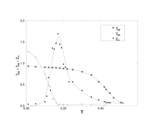
FIG. 5.: Temperature dependence of spin stiffness and chiral susceptibility through the CL transition line of the phase diagram in Fig. 4 at $\rho=0.4$. The data points for $\gamma_{xx}$ are scaled by $10$ and for $\chi_{\sigma}$ scaled by $1/10$.

B Critical exponents

There have been recently many attempts to obtain improved estimates of the critical exponents for the fully frustrated XY model [21, 9, 10, 11, 12]. For the continuous symmetry, the available scaling forms requires the simultaneous fit of two or more parameters and an assumption of KT behavior. This may lead to systematic errors in the location of the KT transition temperature. For the chiral ( Ising-like) order parameter there exist scaling analysis which do not require a precise knowledge of the bulk $T_{c}$ and can provide an estimate of the critical exponents with a one-parameter fit. As simple estimates of $T_{I}$ and $T_{KT}$ already agree within errorbars along the transition line for $\rho>\rho_{L}$, as indicated in Fig. 4, attempting to locate the transition line using, separately, KT scaling forms for the $U(1)$ symmetry and pure Ising critical behavior for the chiral variables will inevitably lead to estimates of critical points which are difficult to resolve on purely numerical grounds due to errorbars. However, if the critical behavior along this line is in fact in the same universality class as the XY-Ising model as suggested by the analysis of Sec. V, then in order to verify the single nature of the transition, it is sufficient to study the $Z_{2}$ degrees of freedom [14]. If the critical exponents are inconsistent with pure Ising values, the transition cannot correspond to the Ising branch of a double transition or to a single but decoupled transition. Moreover, the value of the critical exponent can be used to verify if indeed the critical behavior corresponds to the critical line of the XY-Ising model. In order to estimate the chiral critical exponents independently of $T_{c}$, we use the same method, based on the finite-size scaling of free energy barriers, which has been applied to the SFXY and TFXY models [15].

In order to obtain good statistics, we consider only systems of size $8$ to $36\times 36$, with typically $6-12\times 10^{6}$ Monte Carlo steps. The simulations were performed near the effective (finite size) critical temperature found in the previous Section. The histogram method is then used to extrapolate the needed quantity for different temperatures in the vicinity of the critical temperature. We follow the same method used in Refs. [15, 9] for the SFXY and TFXY models. The thermodynamic critical temperature $T_{c}$ can be determined by the crossing of the free-energy barriers $\Delta F(T,L)$, obtained from the chirality histogram $N(\sigma)$ as $\Delta F=A_{M}(T,L)-A_{m}(T,L)$, where $A_{M}$ is the maximum and $A_{m}$ one of the two minima in $A(\sigma)=-\log N(\sigma)$. At the critical point $\Delta F$ is scale invariant but sufficiently close to $T_{c}$, $\Delta F$ can be expanded to linear order in $tL^{1/\nu}$ as $\Delta F=a+btL^{1/\nu}$, where $t=(T-T_{c})/T_{c}$. In this scaling regime, the exponent $\nu_{I}$ can be extracted from the finite-size behavior of the temperature derivative $\frac{\partial\Delta F}{\partial T}=bL^{1/\nu}$ as a one-parameter fit in a log-log plot, without requiring a precise (simultaneous) determination of $T_{c}$. The exponent $2\beta/\nu$ is extracted from the scaling behavior of $\sigma_{min}\sim L^{-\beta/\nu}$, corresponding to the minimum $A_{m}(\sigma_{\min})$, which only holds at the critical point and thus is more affected but the estimate of $T_{c}$.

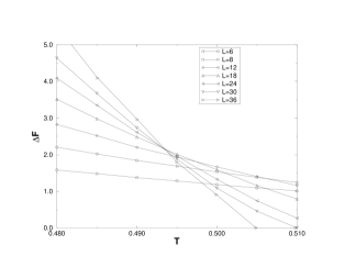
FIG. 6.: Finite-size scaling of the free energy barrier $\Delta F$ for $\rho=1.5$.

We have studied two different values of $\rho$ in detail, $\rho=0.7$ and $\rho=1.5$, which are located between the SFXY model limit and the Lifshitz point and between the SFXY model and the TFXY model limit, respectively. For $\rho=1.5$ we observed crossing of $\Delta F$ for $L\geq 18$ as shown in Fig. 6. Corrections to scaling are clearly seen for $6\leq L\leq 12$. These sizes were not used for the estimates of critical exponents. Note that, this free energy barriers suffer less from corrections to scaling than Binder’s cumulant [32], $U_{L}=1-<\sigma_{L}^{4}>/3<\sigma_{L}^{2}>^{2}$, which is also expected to cross at a unique point. This is shown in Fig. 7 where a sign of unique crossing is only observed at the largest system sizes. The latter behavior has been used by Olsson [8] in relation to the SFXY model to suggest that there are in fact two separate transitions and the estimates of $\nu$ are still dominated by small system sizes. The method we are using, however, indicates clearly a single crossing point suggesting a reliable estimate of $\nu_{I}$. Fig. 8 shows the size dependence of the slope $\frac{\partial\Delta F}{\partial T}|_{T_{c}}$ from where $1/\nu=1.25(1)$ can be estimated and Fig. 9 shows the behavior of $\sigma_{min}$ which gives the estimate $2\beta/\nu=0.29(2)$. The critical temperature is obtained from the value of $T$ at the crossing point in Fig. 7 and gives $T_{c}=0.4935(5)$. The same analysis has been done for $\rho=0.7$ giving $T_{c}=0.408(2)$, $1/\nu=1.28(2)$ and $2\beta/\nu=0.32(4)$. These estimates deviate significantly from the pure Ising values, $1/\nu=1$ and $2\beta/\nu=1/4$, and suggest a single transition scenario. Moreover, these values are consistent with those found for the XY-Ising model along the critical line [15, 16]. This is the same behavior found for the SFXY and TFXY models using the same methods [15].

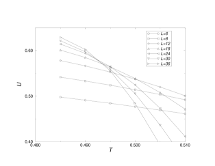
FIG. 7.: Finite-size scaling of Binder’s cumulant $U_{L}$ for $\rho=1.5$.

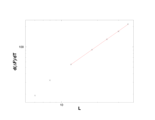
FIG. 8.: Finite-size scaling of $\frac{\partial\Delta F}{\partial T}$ for $\rho=1.5$.

FIG. 9.: Finite-size scaling of $\sigma_{min}$ for $\rho=1.5$.

VII Conclusion

We have introduced a new generalized version of the square-lattice frustrated XY model where unequal ferromagnetic and antiferromagnetic couplings are arranged in a zig-zag pattern. One of the main features of the model is that the ratio between the couplings $\rho$ can be used to tune the system through different phase transitions and in one particular limit it is equivalent to the isotropic triangular-lattice frustrated XY model. The model can be physically realized as a Josephson-junction array with two different couplings and in a magnetic field corresponding to a half-flux quanta per plaquette. We used a mean-field approximation, Ginzburg-Landau expansion and finite-size scaling of Monte Carlo simulations to study the phase diagram and critical behavior. Mean-field approximation gives a phase diagram which qualitatively agrees with the one obtained by Monte Carlo simulations. Depending on the value of $\rho$, two separate transitions or a transition line with combined $Z_{2}$ and $U(1)$ symmetries, takes place. Based on an effective Hamiltonian, we showed that this transition line is in the universality class of the XY-Ising model and the phase transitions of the standard SFXY and TFXY models correspond to two different cuts through the same transition line. Estimates of the chiral ($Z_{2}$) critical exponents from a finite-size analysis of Monte Carlo data were found to be consistent with previous estimates for the SFXY and TFXY models using the same methods. They also agree with the corresponding values along the critical line of the coupled XY-Ising model suggesting a possible physical realization of the XY-Ising model critical line in a frustrated XY model or Josephson-junction array with a zig-zag coupling modulation.

The mean field equations for the zig-zag model can be derived by an analysis similar to the one used in Ref. [19]. The corresponding MF equations are

$$M_{i}\equiv\left\langle\vec{S}_{i}\right\rangle_{MF}=R(\beta H_{i})\frac{\vec{H}_{i}}{H_{i}},$$ (13)

where $\vec{H}_{i}=\sum_{j}J_{ij}\vec{M}_{j}$ is the mean field, $R(x)=I_{1}(x)/I_{0}(x)$ and $\beta=1/kT$ .

To find the MF phase diagram we expand (13) about the transition temperature $T_{c}^{MF}$ using $R(x)=\frac{1}{2}x+O(x)$ for $x\rightarrow 0$, which reduces to

$$\vec{M}_{i}=\frac{1}{2}\frac{1}{T_{c}^{MF}}\sum_{j}J_{ij}\vec{M}_{j}.$$ (14)

It appears that one needs to make an assumption on the form of the solution $M_{i}$ in order to find $T_{c}^{MF}$. However, if we note the similarity of Eq. (14) and the zero temperature limit of Eq. (13), we can identify the transition temperature as

$$T_{c}^{MF}=\frac{H^{GS}}{2},$$ (15)

provided the local field $H_{i}=\sum_{j}J_{ij}\vec{M}_{j}$ is independent of the position. Although this property is not expected to hold in general, it is satisfied exactly in the ground state found in Sec. III. We then obtain

$$\rho \leq \frac{1}{3}\rightarrow T_{c}^{MF}=(-\rho+3)/2$$ (16)

$$\rho \geq \frac{1}{3}\rightarrow T_{c}^{MF}=\sqrt{\left(1+\rho\right)^{3}/4\rho}$$ (17)

If, in addition, we assume that $H_{i}$ remains independent of $i$ at any temperature $0<T<T_{c}^{MF}$ we obtain

$$\frac{R(\beta H)}{H}=\frac{1}{H^{GS}}.$$ (18)

This equation, together with Eq. (13), shows that the structure of the local configuration around a plaquette and the pitch of the helical configuration is independent of the temperature in this approximation.

For $\rho\rightarrow+\infty$ we expect to retrieve the mean field solution of the TFXY model. However Eq. (16) leads to a diverging value of $T_{c}^{MF}$ as $\rho\rightarrow+\infty$. As can be seen from Eq. (13), the temperature is scaled by the magnitude of the mean field vector $(\left|\sum_{j}J_{ij}\vec{M}_{j}\right|)$ which diverges when $\rightarrow+\infty$. This is an artifact of the mean field approximation and other methods, such as perturbative or variational approximation [24] , can remove this divergence. In fact, the phase diagram obtained by Monte Carlo simulations in Sec. V leads to a transition temperature that saturates, for $\rho\rightarrow+\infty$, to a value consistent with the transition temperature of the TFXY model.

REFERENCES

- [1] S. Teitel and C. Jayaprakash, Phys. Rev. B 27, 598 (1983); Phys. Rev. Lett. 51, 199 (1983).
- [2] T.C. Halsey, J. Phys. C 18, 2437 (1985); S.E. Korshunov and G.V. Uimin, J. Stat. Phys. 43, 1 (1986).
- [3] E. Granato, J.M. Kosterlitz, and M.P. Nightingale, Physica B 222, 266 (1996).
- [4] J. Villain, J. Phys. C 10, 1717 (1977).
- [5] S. Miyashita and H. Shiba, J. Phys. Soc. Jpn. 53, 1145 (1984).
- [6] D.H. Lee, J.D. Joanopoulos, J.W. Negele, and D.P. Landau, Phys. Rev. B 33, 450 (1986).
- [7] G. Grest, Phys. Rev. B39, 9267 (1989).
- [8] P. Olsson, Phys. Rev. Lett. 75, 2758 (1995).
- [9] J. Lee, J.M. Kosterlitz and E. Granato, Phys. Rev. B 43, 11531 (1991).
- [10] G. Ramirez-Santiago and J.V. José, Phys. Rev. Lett. 68, 1224 (1992); Phys. Rev. B49, 9567 (1994).
- [11] E. Granato and M.P. Nightingale, Phys. Rev. B 48, 7438 (1993).
- [12] Y.M.M. Knops, B. Nienhuis, H.J.F. Knops and H.W.J. Blöte, Phys. Rev. B 50, 1061, (1994).
- [13] E. Granato, J. Phys. C 20, L215 (1987).
- [14] E. Granato, J.M. Kosterlitz, J. Lee and M.P. Nightingale, Phys. Rev. Lett. 66, 1090 (1991).
- [15] J. Lee, E. Granato and J.M. Kosterlitz, Phys. Rev. B 44, 4819 (1991).
- [16] M.P. Nightingale, E. Granato and J.M. Kosterlitz, Phys. Rev. B52, 7402 (1995).
- [17] B. Berge, H.T. Diep, a. Ghazali, and P. Lallemand, Phys. Rev. B 34, 3177 (1986).
- [18] E. Granato, J.M. Kosterlitz, Phys. Rev. B33, 4767 (1986); J. Phys. C 19, L59 (1986); J. Appl. Phys. 64, 5636 (1988).
- [19] M. Gabay, T. Garel, G.N. Parker, and W.M. Saslow, Phys. Rev. B 40, 264 (1989).
- [20] H. Eikmans, J.E. van Himbergen, H.J.F. Knops and J.M. Thijssen, Phys. Rev. B39, 11759 (1989).
- [21] J.M. Thijssen and H.J.F. Knops, Phys. Rev. B 42, 2438 (1990).
- [22] W.-M. Zhang, W.M. Saslow, M. Gabay, and M. Benakli, Phys. Rev. B 48, 10204 (1993).
- [23] G. André, R. Bidaux, J.-P. Carton, R. Conte, and L. de Seze, J. Physique 40, 479 (1979).
- [24] M. Benakli, H. Zheng and M. Gabay, cond-mat/9609269, to appear in Phys. Rev. B.
- [25] T. Garel and S. Doniach, J. Phys. C 13, L887 (1980).
- [26] W.M. Saslow, M. Gabay, and W.-M. Zhang, Phys. Rev. Lett. 24, 3627 (1992).
- [27] M. Benakli, Ph.D.-thesis, university of Orsay, France, 1995.
- [28] M. Benakli, M. Gabay and W.M. Saslow, unpublished.
- [29] M.Y. Choi and S. Doniach, Phys. Rev. B 31, 4516 (1985).
- [30] H. Kawamura, Phys. Rev. B 38, 4916 (1988).
- [31] M. Yosefin and E. Domany, Phys. Rev. B 32, 1778 (1985).
- [32] K. Binder, Phys. Rev. Lett. 47, 693 (1981).