Abstract

We present a semiclassical two–fluid model for an interacting Bose gas confined in an anisotropic harmonic trap and solve it in the experimentally relevant region for a spin–polarized gas of ⁸⁷Rb atoms, obtaining the temperature dependence of the internal energy and of the condensate fraction. Our results are in agreement with recent experimental observations by Ensher et al..

3 Internal energy and condensate fraction of a trapped interacting Bose gas

Bose–Einstein condensation (BEC) has recently been realized in dilute vapours of spin–polarized alkali atoms, using advanced techniques for cooling and trapping[1, 2, 3, 4, 5]. These condensates consist of several thousands to several million atoms confined in a well which is generated from nonuniform magnetic fields. The confining potential is accurately harmonic along the three Cartesian directions and has cylindrical symmetry in most experimental setups.

The determination of thermodynamic properties such as the condensate fraction and the internal energy as functions of temperature is at present of primary interest in the study of these condensates[4, 5]. The nature of BEC is fundamentally affected by the presence of the confining potential[6] and finite size corrections are appreciable, leading for instance to a reduction in the critical temperature[7, 8, 9, 10]. Interaction effects are very small in the normal phase but become significant with the condensation–induced density increase. The correction to the transition temperature due to interactions has been recently computed by Giorgini et al.[11].

The temperature dependence of the condensate fraction was recently measured[5] for a sample of around 40000 ⁸⁷Rb atoms, the observed lowering in transition temperature being in agreement with theoretical predictions within experimental resolution. In the same work the internal energy was measured during ballistic expansion and found to be significantly higher in the BEC phase than predicted by the ideal–gas model. While the increase is easily understood as a consequence of the interatomic repulsions, a quantitative estimate is still lacking.

In this work we present a two–fluid mean–field model which is able to explain the above–mentioned effects, giving results in agreement with experiment for both the condensate fraction and the internal energy as functions of temperature.

We describe the condensate by means of the Gross–Pitaevskii (GP) equation for its wave function $\Psi(r)$,

$$-{\hbar^{2}\nabla^{2}\over 2m}\Psi(r)+V^{\mathrm{ext}}(r)\Psi(r)+2gn_{1}(r)\Psi(r)+g\Psi^{3}(r)=\mu\Psi(r)$$ (1)

where $g=4\pi\hbar^{2}a/m$, $a$ being the scattering length, $V^{\mathrm{ext}}({\bf r})=m\omega^{2}(x^{2}+y^{2}+\lambda^{2}z^{2})/2$ is the confining potential and $n_{1}(r)$ is the average non–condensed particle distribution. The factor $2$ in the third term arises from exchange[12] and we neglect the term involving the off–diagonal density of non–condensed particles. Following Bagnato et al.[13] we treat the non–condensed particles as non–interacting bosons in an effective potential $V^{\mathrm{eff}}(r)=V^{\mathrm{ext}}(r)+2gn_{1}(r)+2g\Psi^{2}(r)$. Thermal averages are computed with a standard semiclassical Bose–Einstein distribution in chemical equilibrium with the condensate, i.e. at the same chemical potential $\mu$. In particular, the density $n_{1}(r)$ is

$$n_{1}(r) = {1\over(2\pi\hbar)^{3}}\int{d^{3}p\over\exp\left\{\left({p^{2}\over 2m}+V^{\mathrm{eff}}(r)-\mu\right)/k_{B}T\right\}-1}$$ (2)

$$= {(mk_{B}T)^{3/2}\over(2\pi)^{3/2}\hbar^{3}}\sum_{j\geq 1}{1\over j^{3/2}}\exp\left\{-j(V^{\mathrm{eff}}(r)-\mu)/k_{B}T\right\}\,.$$

We fix the chemical potential from the total number of particles $N$

$$N=N_{0}+\int{\rho(E)dE\over\exp\left\{\left(E-\mu\right)/k_{B}T\right\}-1}$$ (3)

where $N_{0}=\int\Psi^{2}(r)d^{3}r$ and the semiclassical density of states is

$$\rho(E)={(2m)^{3/2}\over 4\pi^{2}\hbar^{3}}\int_{V^{\mathrm{eff}}(r)<E}\sqrt{E-V^{\mathrm{eff}}(r)}d^{3}r\,.$$ (4)

This completes the self–consistent closure of the model.

Equation (1) can be solved analytically in the experimentally relevant situation $N\sim 10^{4}\div 10^{5}$ and $a/a_{\perp}\sim 10^{-2}$, where $a_{\perp}=\sqrt{\hbar/m\omega}$. Except for a small region close to the phase transition the interaction parameter $N_{0}a/a_{\perp}$ entering the GP equation is large and the kinetic energy can be neglected. This yields

$$\Psi^{2}(r)={\mu-V^{\mathrm{ext}}(r)-2gn_{1}(r)\over g}\theta(\mu-V^{\mathrm{ext}}(r)-2gn_{1}(r))$$ (5)

where $\theta(x)=0$ ($1$) for $x<0$ ($x>0$). The present strong–coupling solution neglects the condensate zero–point energy $E_{0}^{c}=\hbar\omega(1+\lambda/2)$. As Giorgini, Pitaevskii and Stringari[11] pointed out finite–size effects are thereby excluded.

Before presenting the complete numerical solution of the self–consistent model defined by equations (2)–(5) and comparing its predictions with existing experimental data[5], we display perturbative solutions at zero– and first–order.

An approximate semi–analytical solution can be obtained by treating perturbatively interactions involving the “dilute gas” of non–condensed particles. To zero order in $gn_{1}(r)$ we have

$$N_{0}=\left(2\mu\over\hbar\omega\right)^{5/2}{a_{\perp}\over 15\lambda a}$$ (6)

and equation (4) gives

$$\fl\rho_{0}(E)={1\over\pi\lambda(\hbar\omega)^{3}}\left[2\sqrt{\mu}\left(E\!-\!\mu\right)^{3/2}+E^{2}\mbox{arctn}{\sqrt{E\!-\!\mu\over\mu}}+(2\mu\!-\!E)^{2}\ln{\sqrt{|E\!-\!2\mu|}\over\sqrt{\mu}\!+\!\sqrt{E\!-\!\mu}}\right]$$ (7)

for $\mu>0$ and

$$\rho_{0}(E)={E^{2}\over 2\lambda(\hbar\omega)^{3}}$$ (8)

for $\mu<0$. The self–consistent zero–order solution is then completed by equation (3). We remark that no assumption of weak interactions within the condensate has been made.

We now proceed to compute the first order correction to the above zero–order solution. We take

$$\Psi^{2}(r)={\mu-V^{\mathrm{ext}}(r)-2gn_{1}(0)\over g}\theta(\mu-V^{\mathrm{ext}}(r)-2gn_{1}(0))$$ (9)

and expand equation (4) to first order in $g[n_{1}(r)-n_{1}(0)]$. The choice of the expansion parameter $g[n_{1}(r)-n_{1}(0)]$ ensures that the perturbative expansion is regular, since the correction to $\rho$ vanishes where the zero–order term vanishes. With the additional approximation $g\Psi^{2}(r)\simeq\mu\theta(\mu)$ in the first–order term we get

$$\rho(E)=\rho_{0}(E\!-\!2gn_{1}(0))+\delta\rho_{1}(E\!-\!2gn_{1}(0)-\mu\theta(\mu))$$ (10)

where

$$\fl\delta\rho_{1}(E)={4\over\sqrt{2\pi}\lambda}{a\over a_{\perp}}\left(k_{B}T\over\hbar\omega\right)^{3/2}\sum_{j\geq 1}{Ee^{j\mu\theta(-\mu)/k_{B}T}\over j^{3/2}(\hbar\omega)^{2}}\left[1-{}_{1}F_{1}\left({3\over 2},2,-j{E\over k_{B}T}\right)\right]$$ (11)

${}_{1}F_{1}$ being the Kummer confluent hypergeometric function. The self–consistent first–order solution is then completed by equation (3).

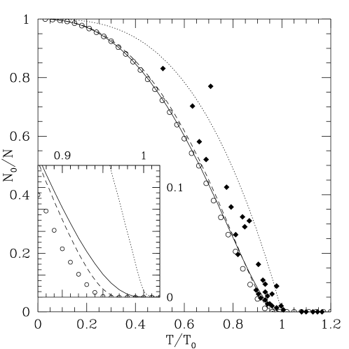
Figure 1: Condensate fraction obtained in the two–fluid model compared with the experimental data of Ensher et al.[5] (diamonds) and with the ideal gas result (dotted curve). We present results obtained from the zero–order solution (full curve), from the first–order perturbative treatment (dashed curve) and from the complete numerical solution (circles). The inset is an enlargement of the region around $T_{\mathrm{c}}$.

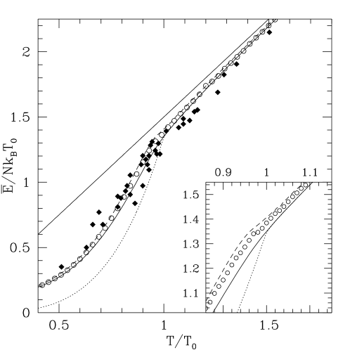
Figure 2: Sum of kinetic and interaction energy, as defined in the text, obtained in the two–fluid model compared with the experimental data of Ensher et al.[5] (diamonds) and with the ideal gas result (dotted curve). We present results obtained from the zero–order solution (full curve), from the first–order perturbative treatment (dashed curve) and from the complete numerical solution (circles). The straight line is the classical Maxwell–Boltzmann result. The inset is an enlargement of the region around $T_{\mathrm{c}}$.

Figure 3: Specific heat $C=d\bar{E}/dT$ obtained in the two–fluid model compared with the ideal gas result (dotted curve). We present results obtained from the zero–order solution (full curve), from the first–order perturbative treatment (dashed curve) and from the complete numerical solution (circles). The straight line is the classical Maxwell–Boltzmann result. The anomalous behaviour obtained from the first–order perturbative solution near $T_{c}$ is an artifact.

We have solved numerically the simplified two–fluid model, first treating the parameter $gn_{1}(0)$ to all orders (equations 2–5), then to zero order (equations 3 and 6–8) and finally to first order (equations 3 and 9–11). Each case involves solving the integral equation (3) to obtain $\mu$ as a function of $N$ and $T$; the non–perturbative solution also involves the local nonlinear problem posed by equations (2) and (5). The small differences between our three results justify a posteriori a perturbative treatment. Experimental parameters are taken from the work of Ensher et al.[5]: $\lambda=\sqrt{8}$, $N=40000$ and $a/a_{\perp}=0.0062$. We have verified numerically that our results depend weakly on $N$ in the region explored in the experiments and therefore have used a fixed $N=40000$ in all our computations. We use as energy units the semiclassical ideal–gas critical temperature $k_{B}T_{0}=\hbar\omega(N\lambda/\zeta(3))^{1/3}$, $\zeta(3)\simeq 1.202$ being the Riemann zeta function.

Figure 1 compares the temperature dependence of the condensate fraction $N_{0}/N$ with the experimental results of Ensher et al.[5]. Lowering of the transition temperature due to interactions is clearly visible, even if the smoothness of our results around the transition prevents a precise assessment of an interaction–induced shift in $T_{\mathrm{c}}$ from the numerical solution. It should be noticed that the strong–coupling solution of the GP equation is not valid for $T$ close to $T_{\mathrm{c}}$, since it requires $N_{0}\gg a_{\perp}/a\simeq 160$, and that our mean field model does not include critical fluctuations. Both effects being relevant only in a narrow window around $T_{\mathrm{c}}$[11], we expect our results to be meaningful in most of the temperature range. Recently Giorgini et al.[11] solved numerically the Popov approximation to the finite–temperature generalization of the GP equation within a semiclassical WKB approximation. Their results for the temperature dependence of the condensate fraction are in very good agreement with the predictions of our more naive model except for $|T-T_{\mathrm{c}}|/T_{\mathrm{c}}<0.05$, where they find a sharp change in the slope of $N_{0}(T)$. Their result for the interaction–induced shift in critical temperature $\delta T_{\mathrm{c}}/T_{\mathrm{c}}\simeq-1.33N^{1/6}a/a_{\perp}\simeq-0.048$ is also in good agreement with our curves.

Figure 2 reports our results for the temperature dependence of the internal energy. We remark that the experimentally measured quantity is the sum of the kinetic energy and of the interaction energy, not including the confinement potential energy due to the rapid switching off of the trapping potential[14]. The average single particle energy ${\langle E\rangle}_{\mathrm{nc}}=\int E\rho(E)dE/\left\{\exp\left[(E-\mu)/k_{B}T\right]-1\right\}$ obtained from the semiclassical density of states contains twice the interaction energy, and – assuming that on average the kinetic and potential terms are equal – is twice the measured quantity. The kinetic energy of condensed atoms is negligible in our strong–coupling limit and their interaction energy per particle is ${\langle E\rangle}_{\mathrm{c}}={1\over 2}g\int\Psi^{4}(r)d^{3}r$. The quantity directly comparable to the experimental data is therefore $\bar{E}=({\langle E\rangle}_{\mathrm{nc}}(N-N_{0})/2+{\langle E\rangle}_{\mathrm{c}})/N$, which we plot in figure 2 obtaining good agreement with the measured values. The calculated internal energy does not contain any sharp feature at transition, paralleling the result discussed above for the condensate fraction. Correspondingly the rapid rise in the specific heat is considerably smoothed with respect to the ideal–gas result (see figure 3). Apart from this small region around transition, our results on $\bar{E}(T)$ above and below $T_{\mathrm{c}}$ imply a significant reduction of the increase in specific heat across the phase transition.

In conclusion, we have presented a mean–field, semiclassical two–fluid model and discussed its perturbative and non–perturbative solution in the experimentally relevant parameter range. Our results on the temperature dependence of the condensate fraction and of the internal energy are in agreement with recent experimental measurements, accounting for the pronounced increase in internal energy with respect to the noninteracting boson case measured below $T_{\mathrm{c}}$. We have also verified that our model reproduces the results obtained for the condensate fraction with a more refined theory by Giorgini et al..

References

References

- [1] Anderson M H, Hensher J R, Matthews M R, Wieman C E and Cornell E A 1995 Science 269 198
- [2] Bradley C C, Sackett C A, Tollett J J and Hulet R G 1995 Phys. Rev. Lett. 75 1687
- [3] Davis K B, Mewes M O, Andrews M R, van Druten N J, Durfee D S, Kurn D M and Ketterle W 1995 Phys. Rev. Lett. 75 3969
- [4] Mewes M O, Andrews M R, van Druten N J, Kurn D M, Durfee D S and Ketterle W 1996 Phys. Rev. Lett. 77 416
- [5] Ensher J R, Jin D S, Matthews M R, Wieman C E and Cornell E A 1996 Phys. Rev. Lett. 77 4984
- [6] De Groot S R, Hooyman G J and ten Seldam C A 1950 Proc. Roy. Soc. London A 203 266
- [7] Grossmann S and Holthaus M 1995 Phys. Lett. A 208 188
- [8] Haugerud H, Haugset T and Ravndal F preprint cond-mat/9605100 (unpublished)
- [9] Minguzzi A, Chiofalo M L and Tosi M P 1997 N. Cimento D (to appear)
- [10] Kirsten K and Toms D J 1996 Phys. Lett. 222A 148
- [11] Giorgini S, Pitaevskii L P and Stringari S 1996 Phys. Rev. A 54 R4633
- [12] Griffin A 1996 Phys. Rev. B 53 9341
- [13] Bagnato V, Pritchard D E and Kleppner D 1987 Phys. Rev. A 35 4354
- [14] Baym G and Pethick C 1996 Phys. Rev. Lett. 76 6