In order to study the effects of strong magnetic field on Kondo insulators, we calculate magnetization curves and single-particle excitation spectra of the periodic Anderson model at half-filling under finite magnetic field by using the self-consistent second-order perturbation theory combined with the local approximation which becomes exact in the limit of infinite spatial dimensions. Without magnetic field, the system behaves as an insulator with an energy gap, describing the Kondo insulators. By applying magnetic field to f-electrons, we found that the energy gap closes and the first order transition from insulator to metal takes place at a critical field $H_{c}$. The magnetization curve shows a jump at $H_{c}$. These are consistent with our previous study in terms of the exact diagonalization. Relationship to the experiments on YbB₁₂ and some other Kondo insulators is discussed.

Keyword: Kondo insulator, insulator-to-metal transition, magnetic field, YbB₁₂

1 Introduction

The materials called as Kondo insulators show the Kondo behavior at high temperatures as typical for the heavy fermion metals, but develop energy gaps at low temperatures. Examples of such materials are SmS,[1] SmB₆,[2] YbB₁₂,[3] TmSe,[4] Ce₃Bi₄Pt₃,[5] etc. The energy gap seems to be formed due to the hybridization of the 4f states with the conduction bands, but it is considered that the strong correlation is playing an important role in determining the size of the gap and the other properties[6]. FeSi is also considered to fall into this family[6]. CeNiSn[7] is believed to have a pseudogap, or even to be a semimetal at lowest temperatures.[8]

In order to know the characters of the energy gap of the Kondo insulators, a stimulating experiment was performed on YbB₁₂ by Sugiyama, et al.[9] In their experiment, the application of a strong magnetic field of about 47T destroys the gap and the system undergoes a transition from insulator to metal. The magnetization starts to steeply increase at a critical field.

It is an interesting theoretical issue to investigate how the strongly renormalized ground state of the Kondo insulators will be modified and how the gap is destroyed by the magnetic field. For these purposes, we previously applied the recently developed techniques to treat the strongly correlated electron systems in the infinite spatial dimensions[10, 11]. In this scheme, the study of the strongly correlated lattice system is reduced to solving the impurity problem in an effective medium self-consistently. Therefore, it is sometimes called as the local-impurity self-consistent approximation or the dynamical mean field theory.[11] We solved the effective impurity problem by the exact diagonalization (EXD) of the finite system for conduction electrons and calculated the single-particle excitation spectra to determine the energy gap.[12, 13, 14] (The paper[12] will be referred to as I in the following.) We found that the gap decreases linearly with the magnetic field and vanishes abruptly at a certain critical field $H_{c}$, which is of the order of the impurity Kondo temperature, and that the insulator-to-metal transition takes place. The magnetization curves exhibit a jump at $H_{c}$. These features suggest that the transition is of first order.

We discussed in I that there are two effects of the magnetic field on the energy gap in the Kondo insulators. One is the Zeeman shift of the up- and down-spin bands, which leads to the closing of the gap. The other is the reduction of the strong renormalization due to correlation, which results in the increase of the renormalization factor $z=(1-\partial\Sigma_{f}(\epsilon)/\partial\epsilon)^{-1}|_{\epsilon=0}$ ($\Sigma_{f}(\epsilon)$ denotes the f-electron self-energy) from $z\ll 1$ to $z\sim 1$. This gives rise to the increase of the gap since the gap $E_{g}$ is estimated to be of the order of $zV^{2}/W$, where $V$ denotes the mixing matrix element and $W$ the conduction band width. We found that at least at half-filling in the symmetric case $z$ does not change by the field as far as $h<h_{c}$. Therefore, the energy gap closes merely by the Zeeman shift of the bands, although an abrupt transition to metal takes place before the gap completely closes in this way. This first order transition may be due to the complicated many-body effects. However, it might be possible that it would be due to the finite size effect of the conduction electron system.

Recently, Carruzzo and Yu[15] and Tsutsui, et al.[16] claimed that the gap remains finite even under strong magnetic field and the field-induced insulator-to-metal transition does not occur in one dimensional Kondo insulators. Their conclusions still seem to be indefinite because of their numerical methods (density matrix renormalization group and exact diagonalization, respectively). However, it is interesting to study whether such transition occurs or not in higher dimensions.

In order to clarify these points, we will use in the present paper the self-consistent second-order perturbation theory (SCSOPT),[17, 18, 19] and reinvestigate the character of the field-induced insulator-to-metal transition in Kondo insulators. As will be explained below, we have found again that the transition does occur and is of first order, so that our previous conclusions mentioned above are correct at least qualitatively. For comparison, a calculation by the iterative perturbation theory[20] (IPT) was also performed, but we found that IPT yields quantitatively insufficient results under finite magnetic field. We will also comment on the possible relationship to the experiments on YbB₁₂ and some other Kondo insulators.

2 Self-consistent Second-order Perturbation Theory and Iterative Perturbation Theory

We use the periodic Anderson model (PAM),

$$H = \sum_{ij\sigma}t_{ij}c_{i\sigma}^{+}c_{j\sigma}+\sum_{i\sigma}E_{f\sigma}f_{i\sigma}^{+}f_{i\sigma}$$

$$+ \frac{V}{\sqrt{N}}\sum_{i\sigma}\Bigl{(}f_{i\sigma}^{+}c_{i\sigma}+h.c.\Bigr{)}+U\sum_{i}\delta n_{fi\uparrow}\delta n_{fi\downarrow},$$ (1)

where $\delta n_{f\sigma}=n_{f\sigma}-\langle n_{f\sigma}\rangle$, $E_{f\sigma}=E_{f}+U\langle n_{f-\sigma}\rangle-\sigma h$, $h=\mu_{B}H$ and $H$ denotes the magnetic field. $N$ is the number of lattice sites. The other notations are standard. We neglect the orbital degeneracy and assume the symmetric case $E_{f}=-U/2$ together with the half-filling condition to express the simplest model to the Kondo insulators. Since the g-factors for f- and the conduction electrons ($g_{c}$ and $g_{f}$, respectively) are different, we neglect $g_{c}$ for simplicity and apply magnetic field only to f-electrons, although a more general treatment is possible.[19] We also assume a paramagnetic ground state. Possible antiferromagnetic states are regarded as being suppressed by the introduction of an appropriate frustration.[21]

In SCSOPT[17], the self-energy is calculated as

$$\Sigma_{f\sigma}(\epsilon) = U^{2}\int d\epsilon_{1}\int d\epsilon_{2}\int d\epsilon_{3}\rho_{\sigma}(\epsilon_{1})\rho_{-\sigma}(\epsilon_{2})\rho_{-\sigma}(\epsilon_{3})$$ (2)

$$\times \frac{f(-\epsilon_{1})f(\epsilon_{2})f(\epsilon_{3})+f(\epsilon_{1})f(-\epsilon_{2})f(-\epsilon_{3})}{\epsilon-\epsilon_{1}+\epsilon_{2}+\epsilon_{3}+i\delta}$$

where $\rho_{\sigma}(\epsilon)=(-1/\pi)\mbox{Im}G_{f\sigma}(\epsilon+i\delta)$ is the f-electron density of states, $f(\epsilon)$ denotes the Fermi function and

$$G_{f\sigma}(\epsilon)=\frac{1}{N}\sum_{k}\frac{1}{\epsilon-E_{f\sigma}-\Sigma_{f\sigma}(\epsilon)-\frac{V^{2}}{\epsilon-\epsilon_{k}}}.$$ (3)

Here $\epsilon_{k}$ denotes the energy of conduction electrons. These equations are converted into the following forms:

$$\Sigma_{f\sigma}(\epsilon) = -iU^{2}\int_{0}^{\infty}\!\!\!dte^{i\epsilon t}\left[\beta_{\sigma}(t)\alpha_{-\sigma}(t)\beta_{-\sigma}(t)\right.$$ (4)

$$+\left.\alpha_{\sigma}(t)\beta_{-\sigma}(t)\alpha_{-\sigma}(t)\right],$$

$$\left.\begin{array}[]{l}\alpha_{\sigma}(t)\\ \beta_{\sigma}(t)\end{array}\right\}=\int_{-\infty}^{\infty}\!\!\!d\epsilon e^{-i\epsilon t}\rho_{\sigma}(\epsilon)f(\pm\epsilon),$$ (5)

$$G_{f\sigma}(\epsilon)=g_{\sigma}(\epsilon)\left[1+V^{2}g_{\sigma}(\epsilon)F(\epsilon-V^{2}g_{\sigma}(\epsilon))\right],$$ (6)

$$g_{\sigma}(\epsilon)=(\epsilon-E_{f\sigma}-\Sigma_{f\sigma}(\epsilon))^{-1}$$ (7)

and

$$F(z) = \sum_{k}(z-\epsilon_{k})^{-1}$$ (8)

$$= (2/W)[z/W-\sqrt{(z/W)^{2}-1}].$$

The last equation was obtained for the semi-circular density of states of the conduction electrons: $\rho(\epsilon)=(2/\pi W)[1-\sqrt{1-(\epsilon/W)^{2}}]$. These equations should be calculated self-consistently.

In IPT,[20] the lattice problem is converted into solving an effective impurity problem, so that $\rho_{\sigma}(\epsilon)$ in eqs.(2) and (5) should be replaced with that for the local Green’s function, $\tilde{\rho}_{\sigma}(\epsilon)=(-1/\pi)\mbox{Im}\tilde{G}_{f\sigma}(\epsilon+i\delta)$, where

$$\tilde{G}_{f\sigma}(\epsilon)=(G_{f\sigma}(\epsilon)^{-1}+\Sigma_{f\sigma}(\epsilon))^{-1}.$$ (9)

3 Results

It is rather easy to solve the above equations self-consistently when $h=0$. We choose $W=1$ as a unit of energy and $V=0.5$. The following calculations are limited to the absolute zero temperature. In Fig.1(a), we compare the f-electron density of states $\rho(\epsilon)$ by IPT for $U=2$ with that obtained in I by EXD using the finite system.[12]

Figure 1: (a) Comparison of the f-electron density of states calculated by the exact diagonalization of the finite system (full lines) and by IPT (broken lines) for $U=0,\ 1,\ 2,\ 3$ (from bottom to top). (b) The f-electron density of states calculated by SCSOPT for the same parameters as in (a). Note that the origins of the vertical axis are shifted.

There are rich structures in $\rho(\epsilon)$ obtained by EXD. In addition to the hybridization-split Kondo peaks at small energies, there are peaks at $\epsilon\sim\pm 0.8$ and $\pm 1.7$ for $U=2$, for instance. The spectra by SCSOPT are displayed in Fig.1(b). The whole structures are better reproduced by IPT than SCSOPT. This is in accord with the results obtained by Mutou and Hirashima[22] on the comparison of the quantum Monte Carlo calculation with IPT and SCSOPT. The peaks at $\epsilon\sim\pm 1.7$ in EXD are the lower and the upper Hubbard bands, which are pushed out a little beyond $\pm U/2$. In SCSOPT, there are only small shoulders at these positions, but it is interesting that there are larger peaks at $\epsilon\sim\pm 0.8$ which correspond to the peaks in EXD at the same positions.

These differences in the spectra in SCSOPT and IPT come from the differences in the self-energies. We have plotted the f-electron self-energies for $U=2$ in Fig.2. It is seen that the absolute values of the real and the imaginary parts of $\Sigma_{f}(\epsilon)$ are larger in ITP than in SCSOPT. This makes the Hubbard bands in IPT be positioned at the right energies and enhanced sufficiently to reproduce the EXD results. The fine structures of the spectra in SCSOPT seen above seem to be originating from the structures in the imaginary part of the self-energy at the corresponding energy regions.

Figure 2: The real and the imaginary parts of the f-electron self-energy calculated by IPT (full and broken lines for real and imaginary parts) and SCSOPT (dash-dotted and dotted lines) for U=2.

Despite the better description of the f-electron density of states in IPT than in SCSOPT, we have found that magnetic properties are better described by SCSOPT (see below). This is because IPT is not a conserving approximation.[19] Therefore, we will use SCSOPT in the following calculations.

Under finite magnetic field, one also has to determine $n_{f\sigma}$ self-consistently. We found, however, that the convergence of the iterative calculation becomes rather poor in the vicinity of the critical field. To overcome this difficulty, we first assume appropriate input values $n_{f\sigma}^{0}$ for $n_{f\sigma}$ and solve the above equations for fixed $E_{f\sigma}$. Then we obtain $G_{f\sigma}(\epsilon)$ and $n_{f\sigma}$ from them. We repeat this calculation for various $n_{f\sigma}^{0}$’s and plot $m=n_{f\uparrow}-n_{f\downarrow}$ vs. $m_{0}=n_{f\uparrow}^{0}-n_{f\downarrow}^{0}$ in Fig.3(a).

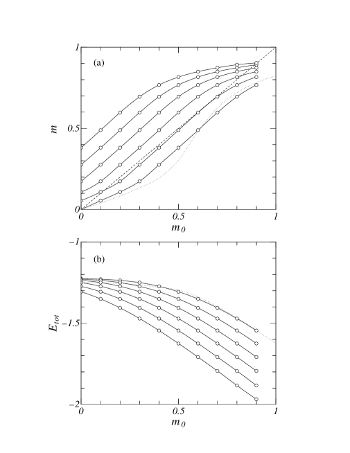
Figure 3: (a) $m$ vs. $m_{0}$ curves (see the text) obtained by SCSOPT for $U=2$ and $h=$0, 0.1, 0.2, 0.3, 0.4, 0.5 from bottom to top. (The IPT result for $h=0$ is displayed by the dotted curve for comparison.) (b) The total energies for the same set of parameters are plotted from top to bottom.

The points of intersection with the line of the slope of 45 degrees give the self-consistent solution $m=m_{0}$. It is clear from the S-like shape of $m$ vs. $m_{0}$ curves that the first order transition takes place at a certain critical field $h_{c}$, which was found to be $h_{c}=0.101$ at $U=2$. We also checked that the total energy,[23]

$$E_{tot} = \sum_{\sigma}\int d\epsilon f(\epsilon)\left(\frac{1}{\pi}\right)\mbox{Im}\Bigl{[}\epsilon G_{c\sigma}(\epsilon)$$ (10)

$$+\left(\epsilon-\frac{1}{2}\Sigma_{f\sigma}(\epsilon)\right)G_{f\sigma}(\epsilon)\Bigr{]},$$

where

$$G_{c\sigma}(\epsilon) = \sum_{k}\frac{1}{\epsilon-\epsilon_{k}-V^{2}/(\epsilon-E_{f\sigma}-\Sigma_{f\sigma}(\epsilon))}$$ (11)

$$= F(\epsilon-V^{2}g_{\sigma}(\epsilon)),$$

is lower for larger $m_{0}$ (Fig.3(b)).

The transition becomes continuous for $U<1.7$ since the S-shape of the $m$ vs. $m_{0}$ curves becomes weak. On the other hand, the ferromagnetic state becomes stable even at $h=0$ for $U>2.6$ because of a stronger S-shape.

The data in Fig.3 are spline-interpolated on $m_{0}$ and $h$, from which we determine the self-consistent solution $m=m_{0}$ with a good accuracy. We plot the magnetization curve in Fig.4. It shows a jump at $h_{c}$ for $1.7<U<2.6$, although the size of the jump is larger than that in EXD. The double steps found by EXD for $U=1$ could be a reminiscence of a change of the character of the transition from first to second order.

IPT also yields S-shape curves in the $m$ vs. $m_{0}$ relations, but the S-shape is stronger than in SCSOPT (see Fig.3(a), the dotted curve), giving smaller $h_{c}$ ($h_{c}=0.071$ for $U=2$). A fatal drawback in IPT is that it gives wrong value for the initial slope of the magnetization curve (i.e. magnetic susceptibility $\chi_{f}$). We found $\chi_{f}=$1.22 and 1.20 in SCSOPT and EXD, respectively, whereas $\chi_{f}=0.67$ in IPT for $U=2$. This discrepancy is due to the fact that IPT is not a conserving approximation[19] as mentioned above.

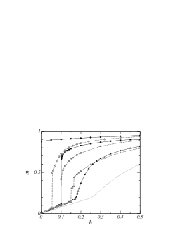
Figure 4: Magnetization curves for $U=$0 (dotted line), 1 (triangles), 2 (squares), 3 (diamonds) calculated by SCSOPT (filled symbols) and EXD (open symbols).

The f-electron densities of states under finite magnetic field are plotted for $U=2$ in Fig.5, from which the energy gaps are obtained and are plotted in Fig.6 as a function of the field. The gap closes abruptly between $h=$0.101 and 0.1015. From these results, we consider that the first order transition obtained in I may not be due to the finite-size effect.

Figure 5: The f-electron density of states for up-spin electrons ($U=2$) under the magnetic field $h=$0, 0.05, 0.101 and 0.1015 from bottom to top.

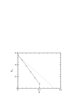
Figure 6: The Energy gap obtained by SCSOPT (circles) as a function of $h$ for $U=2$. The dotted line indicates the gap for $U=0$ scaled at $h=0$.

Finally, we would like to comment on the behavior of the self-energy in the magnetic field. Fig.7 shows the field dependence of the real part of the self-energy. As is seen clearly, Re$\Sigma_{f\sigma}(\epsilon)$ does not depend on $h$ when $h<h_{c}$. This is because the shift of $\rho_{\sigma}(\epsilon)$’s in eq.(2) by the magnetic field does not yield a noticeable change of $\Sigma_{f\sigma}(\epsilon)$ until the gap is closed by the sufficient field. Due to this behavior in the self-energy, the renormalization factor $z$ changes little for $h<h_{c}$. Thus the gap closing is mainly caused by the relative Zeeman shift of up- and down-spin bands. Note that the gap does not close like $E_{g}(h)=E_{g}(0)-2h$ even for $U=0$ since we apply magnetic field only to f-electrons, so that the shape of $\rho_{\sigma}(\epsilon)$ canges with the field. The energy gap for $h=0$ is given by $E_{g}(0)=-W+\sqrt{W^{2}+4V^{2}}=0.414$ for $W=1$ and $V=0.5$, whereas $h_{c}$ is given by $h_{c}=V^{2}/W=0.25$, which is larger than $E_{g}(0)/2$. We have plotted $E_{g}(h)$ for $U=0$ in Fig.6 by the dotted line, which is scaled at $h=0$. The gap by SCSOPT decreases a little faster than that for $U=0$, which means that the shape of $\rho_{\sigma}(\epsilon)$ at $U=2$ changes more than that of $U=0$ by the field despite the small change of $z$.

Figure 7: The real parts of the self-energy are plotted for $h=$0 (full line), 0.05 (dashed line), 0.101 (broken line) and 0.1015 (dotted line).

4 Discussions

We have found that the energy gap in Kondo insulators is closed by the application of a sufficiently strong magnetic field of the order of the gap, and a transition from insulator to metal does take place in the limit of infinite spatial dimensions. This is in strong contrast to the suggestions for the one dimensional Kondo insulators.[15, 16] We found that the transition is of first order, and the magnetization shows a jump at the critical field $h_{c}$, irrespective of the methods of calculations, although the first order transition is limited to the range $1.7<U<2.6$ in SCSOPT. The calculation was only for the electron-hole symmetric case. It is of much interest to extend the present calculation to more general situations and to more realistic models with orbital degeneracy. We started from a paramagnetic ground state, assuming that a frustration should have destroyed a long range order.[21] It is necessary, however, to extend the calculation to such an explicit model which has a paramagnetic ground state.

Despite these issues to be clarified in future studies, we stress that the magnetic-field-driven insulator-to-metal transition is of great interest and importance for the study of the characters of the Kondo insulators since a sufficiently strong magnetic field always tends to close the gap. On the other hand, the pressure, for instance, sometimes increases the mixing and the gap, but in some other cases increases the band width, causing the overlapping of the band and rendering the system semimetallic. In this sense, the magnetic field is much simpler and a good tool for the study of the insulator-to-metal transition in strongly correlated electron systems.

First order transition has not yet been observed in YbB₁₂. This is partly because the energy gap was determined from the temperature dependence of the resistivity, so that the finite temperature might have smeared out the transition, or the system is out of range of the first order transition. More direct experiments at low temperatures, e.g. measurement of the dynamical conductivity, etc. are desirable. Lacerda applied the magnetic field of up to 50T to SmB₆ and did not find any indication of a transition to metal.[24] This may be because of the smaller magnetic moment for Sm ($gJ=2.14$ for Ce whereas $gJ=0.71$ for Sm). Magnetoresistance of CeNiSn is measured to be positive[8] in contrast to the present calculation. The structure of the gap and the mechanism of the low temperature transport in this compound is still not clear. However, the effect of the magnetic field on the strongly correlated state should be different if the gap is of V shape. Study of such situation will be interesting also from the present theoretical point of view.

Recently, a new IPT scheme was proposed[25, 26], which can be applied even to the case without electron-hole symmetry. It may be applicable to a calculation of the properties of the strongly correlated systems under magnetic field, and may improve the present calculation, including the cases with larger $U$ and the study of metamagnetism in the metallic heavy fermion systems.

References

- [1] A. Jayaraman, V. Narayanamurthi, E. Bucher and R. G. Maines: Phys. Rev. Lett. 25 (1970) 1430.
- [2] A. Menth, E. Buehler and T. H. Geballe: Phys. Rev. Lett. 22 (1969) 295.
- [3] M. Kasaya: J. Mag. Magn. Mater. 47 & 48 (1985) 429.
- [4] P. Haen, F. Lapierre, J. M. Mignot, R. Tournier and F. Holtzberg: Phys. Rev. Lett. 43 (1979) 304.
- [5] M. F. Hundley, P. C. Canfield, J. D. Thompson, Z. Fisk and J. M. Laurence: Phys. Rev. B42 (1990) 4862.
- [6] G. Aeppli and Z. Fisk: Comments Cond. Mat. Phys. 16 (1992) 155.
- [7] T. Takabatake, F. Teshima, H. Fujii, S. Nishigori, T. Suzuki, Y. Yamaguchi, J. Sakurai and D. Jaccard: Phys. Rev. B41 (1990) 9607.
- [8] G. Nakamoto, T. Takabatake, H. Fujii, A. Minami, K. Maezawa, I. Oguro, and A. A. Menovsky: J. Phys. Soc. Jpn. 64 (1995) 4834.
- [9] K. Sugiyama, F. Iga, M. Kasaya, T. Kasuya and M. Date: J. Phys. Soc. Jpn. 57 (1988) 3946.
- [10] W. Metzner and D. Vollhardt: Phys. Rev. Lett. 62 (1989) 324.
- [11] A. Georges, G. Kotliar, W. Krauth and M. J. Rozenberg: Rev. Mod. Phys. 68 (1996) 13.
- [12] T. Saso and M. Itoh: Phys. Rev. B53 (1996) 6877.
- [13] T. Saso: to appear in Physica B (1996).
- [14] T. Saso: Czechoslovak Journal of Physics 46 (1996) 2637.
- [15] H. M. Carruzzo and C. C. Yu: Phys. Rev. B53 (1996) 15377.
- [16] K. Tsutsui, Y. Ohta, R. Eder, S. Maekawa, E. Dagotto and J. Riera: to appear in Proceedings of SCES96, Physica B (1996).
- [17] E. Müller-Hartmann: Z. Phys. 76 (1989) 211.
- [18] H. Schweizer and G. Czycholl: Z. Phys. 79 (1990) 377.
- [19] T. Mutou and D. S. Hirashima: J. Phys. Soc. Jpn. 63 (1994) 4475.
- [20] A. Georges and G. Kotliar: Phys. Rev. B45 (1992) 6479.
- [21] M. J. Rozenberg, G. Kotliar and X. Y. Zhang: Phys. Rev. B49 (1994) 10181.
- [22] T. Mutou and D. S. Hirashima: J. Phys. Soc. Jpn. 64 (1995) 4799.
- [23] A. L. Fetter and J. D. Walecka: Quantum Theory of Many-Particle Systems (McGraw Hill, 1971).
- [24] A. Lacerda, J. D. Gettee, G. M. Schmiedeshoff, A. Kebede and J. L. Smith: Czechoslovak Journal of Physics 46 (1996) 1991.
- [25] H. Kajueter and G. Kotliar: Phys. Rev. Lett. 77 (1996) 131.
- [26] H. Kajueter, G. Kotliar and G. Moeller: Phys. Rev. B53 (1996) 16214.