[

Bose glass and Mott insulator phase in the disordered boson Hubbard model

Abstract

We study the Villain representation of the two-dimensional disordered boson Hubbard model via Monte Carlo simulations. It is shown that the probability distribution of the local susceptibility has a $1/\chi^{2}$-tail in the Bose glass phase. This gives rise to a divergence although particles are completely localized here as we prove with the help of the participation ratio. We demonstrate the presence of an incompressible Mott lobe within the Bose glass phase and show that a direct Mott-insulator to superfluid transition happens at the tip of the lobe. Here we find critical exponents $z=1$, $\nu\sim 0.7$ and $\eta\sim 0.1$, which are reminiscent of the pure three-dimensional classical XY model.

]

At zero temperature two-dimensional systems of interacting bosons can show a quantum phase transition from an insulating phase to a superconducting phase [1, 2]. Such a transition can be observed experimentally in granular superconductors [3] and in ⁴He-films absorbed in arogels [4]. By tuning a control parameter like the disorder strength or the chemical potential the bosons become localized in a so called Bose glass phase that is insulating but gapless and compressible. A huge theoretical effort has been undertaken to shed like on the universal properties of this superconductor-to-insulator transition. In two dimensions the model has eluded successful analytical treatment, which necessitates numerical methods as quantum Monte Carlo simulations [5, 6, 7, 8, 9], real space renormalization group calculations [10] or strong coupling expansion [11].

Apart from this generic transition the Bose glass phase itself has a number of universal features that are relevant for experiments. Since it is gapless various zero-frequency susceptibilities will diverge [2], which is reminiscent of the quantum Griffiths phase occuring in random transverse Ising systems [13, 14, 15, 16, 17], where a continuously varying dynamical exponent parametrizes the occuring singularities. Moreover, for weak disorder a different transition, directly from a superconducting to a Mott-insulating phase might occur [10, 6]. This scenario emerges also from recent theoretical considerations [12] and would establish a new universality class different from the one investigated in [5, 7, 8, 9].

In this letter we address these two questions in a numerical approach. We report on results obtained by extensive quantum Monte Carlo simulations of the disordered boson Hubbard model (BH) with short range interactions in two dimensions, which is defined by

$$H=-t\sum_{\langle ij\rangle}(a_{i}^{+}a_{j}+a_{i}a_{j}^{+})+\frac{U}{2}\sum_{i}n_{i}^{2}-\sum_{i}\mu_{i}n_{i}$$ (1)

where $\langle ij\rangle$ are nearest neighbor pairs on a square lattice, $a_{i}^{+}$ ($a_{i}$) are boson creation (annihilation) operators, $n_{i}=a_{i}^{+}a_{i}$ counts the number of bosons at site $i$, $U$ is the strength of an on-site repulsion and $\mu_{i}$ is a random chemical potential. We are interested in the ground state properties (i.e. at temperature $T=0$) of (1). By using standard manipulations [7] we rewrite the ground state energy density of (1) as a free energy density of a classical model

$$f=-\frac{1}{L^{2}L_{\tau}}\,\ln\,\sum_{\{\bf J\}}^{\nabla\cdot{\bf J}_{i,t}=0}\,\exp(-S\{{\bf J}\})\;,$$ (2)

where the integer current variables $J_{i,t}^{x}$, $J_{i,t}^{y}$ and $J_{i,t}^{\tau}$, live on the links of a (2+1)-dimensional cubic lattice of linear size $L$ in the two space directions (with coordinates $i=(x,y)$) and $L_{\tau}\propto 1/T$ in the (imaginary) time direction (with coordinate $t$). Ultimately one has to perform the limit $L_{\tau}\to\infty$ (i.e. $T\to 0$). The current vector ${\bf J}_{i,t}=(J_{i,t}^{x},J_{i,t}^{y},J_{i,t}^{\tau})$ has to be divergenceless on each lattice site $(i,t)$ as indicated. The classical action $S$ is given by

$$S\{{\bf J}\}=\frac{1}{K}\sum_{(i,t)}\left\{\frac{1}{2}{\bf J}^{2}_{i,t}-(\mu+v_{i})J^{\tau}_{i,t}\right\}\;.$$ (3)

The coupling constant $K$ acts as a temperature and corresponds to $t/U$. Note that the mapping from (1) to (3) involves various approximations [7] and we stress right from the beginning that we report exclusively on results for the classical model (3). However, as far as universal properties are concerned, we expect them to be valid also for (1). The random part $v_{i}$ of the local chemical potential is distributed uniformly between $-\Delta$ and $+\Delta$. All results are disorder averages over at least 500 samples, obtained by Monte Carlo simulations of the classical model (3) with an appropriate heat bath algorithm [7] at classical temperature $K$. Details of the calculations will be published elsewhere [18].

In mean field theory one expects the following $K-\mu$ phase diagram [2]: For $\Delta<0.5$ there is a superfluid (SF) phase at large $K$, a Bose glass (BG) phase at small $K$ and a sequence of Mott-insulator (MI) lobes embedded into the BG phase centered around $K=0$, $\mu$ integer. For $\Delta\geq 0.5$ the Mott lobes vanish and only the BG and SF phases remain. In this case the SF-BG transition is generic everywhere along the phase separation line and has been investigated extensively in [7] in two dimensions at the point $K=K_{c}(\Delta=0.5,\mu=0.5)$. The nature of the transition at the tip of the Mott lobes (i.e. at $\mu=n$ and $K=K_{c}^{\prime}(\Delta,n)$ for $\Delta<0.5$) is not clear and under discussion in the literature [2, 10, 5, 6, 11].

Our first goal is to shed light on the Bose glass phase itself. It has been argued [2] that here the density of states at zero energy does not vanish, leading to a divergent superfluid susceptibility, although the correlation length is finite. On one hand, this behavior is reminiscent of the quantum Griffiths phase in random transverse Ising systems [14, 15, 16]. On the other hand we demonstrate in this letter that the BG phase is different from the Griffiths phase in the following respect: whereas in the latter strongly coupled clusters lead to a divergence of varying strength with varying coupling constant, essentially fully localized excitations give rise to a uniform, logarithmic divergence in the former.

We study the local superfluid susceptibility, which is defined by $\chi_{i}=\sum_{t=1}^{L_{\tau}}C_{i}^{+}(t)$ with the imaginary time autocorrelation function $C_{i}^{+}(t)=\langle\exp\{-\frac{1}{K}\sum_{t^{\prime}=1}^{t}(1/2+J^{\tau}_{i,t^{\prime}}-\mu_{i})\}\rangle$ where the angular brackets $\langle\cdots\rangle$ mean a thermodynamic average. Note that $C_{i}^{+}(\tau)$ corresponds to the local (imaginary time) Greens function $\langle a_{i}(\tau)a_{i}^{+}(0)\rangle$ in the original BH model (1) and the local susceptibility is simply its (zero frequency) integral.

FIG. 1.: The probability distribution $P(\ln\chi_{\rm loc})$ of the local susceptibility for various values of $K$ ($\Delta=0.5$, $\mu=0.5$, the BG-SF transition is at $K_{c}=0.247$). The system size is $L=6$ and $L_{\tau}=200$. For $K=0.19$, which is deep in the Bose glass phase, also data for $L=4$ and $L=10$ are shown, which is indistinguishable from $L=6$.

The probability distribution $P(\ln\chi)$ is shown in fig. 1 for the case $\Delta=0.5$, from which we conclude that

$$\ln\,P(\ln\chi)=-\frac{d}{z}\ln\chi+const.$$ (4)

with $z=d=2$ throughout the BG phase. We have chosen the notation of ref. [16, 15] in order to demonstrate that the dynamical exponent $z$ that is characteristic for a Griffiths phase [13] in random transverse Ising models can also be defined in the present context and is constant here. Note that here $z=d$ in the BG phase and at the critical point, although the two exponents have their origin in different physics [20]. We also looked at weaker disorder $\Delta=0.2$, where MI lobes are present. As soon as one enters the latter, the distribution $P(\chi)$ is chopped off at some characteristic value inversely proportional to the non-vanishing gap in the MI phase. This implies furthermore that the BG phase is indeed gapless [2].

FIG. 2.: The participation ratio $p_{L}(K)$ (5) as a function of $K$ for various system sizes ($\Delta=0.5$, $\mu=0.5$). Within the Bose glass phase ($K<K_{c}=0.247$) $p_{L}$ approaches a constant. The insert shows a scaling plot with $\nu=0.9$ and $y=1.0$.

The relation (4) could be obtained by setting the hopping matrix element $t$ to zero in (1), which yields a completely local Hamiltonian. This lets us suspect that the fact that $z$ does not vary within the BG phase is due to the local nature of the low lying excitations. To further clarify this point we try to quantify the degree of localization of the latter. However, since it is not possible to obtain these excitations directly in the representation we use, we introduce a participation ratio [21]

$$p_{L}=\left[\sum_{i=1}^{N}\langle\rho_{i}\rangle^{2}\right]_{\rm av}^{-1}$$ (5)

for the spatial density distribution $\rho_{i}=L_{\tau}^{-1}\sum_{t}(J_{i,t}^{\tau,b}-J_{i,t}^{\tau,a})$ of an additional particle, i.e. here we work with two replicas $\alpha$ and $\beta$ of the system, one with fixed particle number $N$ and the other with $N+1$ ($N=L^{2}/2$ for the transition that corresponds to $\mu=1/2$). $[\cdots]_{\rm av}$ denotes a disorder average. One expects $p_{L}={\cal O}(1)$ if the extra particle is localized and $p_{L}={\cal O}(N)$ if it is delocalized. The result is shown in fig. 2, where we see very clearly, that the additional particle becomes completely localized within the BG phase, most probably at those sites, which allow for an extra particle, i.e. $v_{i}\approx 0$ (since we are at $\mu=1/2$). Moreover the insert shows that $p_{L}(K)$ satisfies the following scaling relation for fixed aspect ratio $L_{\tau}/L^{z}$ at the generic SF-BG transition

$$\frac{p_{L}(K)}{L^{2}}=L^{-y}\tilde{q}(\delta L^{1/\nu})\;,$$ (6)

with $\delta=(K-K_{c})/K_{c}$ the distance from the critical point ($K_{c}=0.247$), $\nu=0.9\pm 0.1$ and $z=2$ as in [7] and $y=1.0\pm 0.1$.

FIG. 3.: The average particle number $n_{i}$ and compressibility $\kappa$ as a function of the chemical potential $\mu$ ($\Delta=0.2$, $K=0.19$). At $\mu=0.5$ one is deep in the Bose glass phase and $n_{i}=1/2$. The lower insert shows the compressibility: for large $L_{\tau}$ the drop in $\kappa$ becomes sharper. The upper insert shows how the plateau (i.e. the Mott lobe) vanishes in the vicinity of $K=K_{c}^{\prime}(\Delta=0.2,\mu=1)$.

Now we consider the MI lobes within the BG phase. We choose $\Delta=0.2$ and explore the MI-BG boundary by varying the chemical potential between $0.5$ and $1.5$ with fixed $K<K_{c}(\Delta=0.2,\mu=0.5)=0.20$. The latter point corresponds to the generic BG-SF transition studied in [7], but now with weaker disorder. We checked that one indeed gets the same critical exponents as for $\Delta=0.5$. In fig. 3 one sees that with increasing $\mu$ the average particle density per site increases monotonically until it saturates in a plateau at $n_{i}=1$. The plateau region indicates the boundary of the MI phase centered around $\mu=1$ with exactly one particle per site. There is only a weak size dependence, at least as long as one is deep inside the BG phase, where the correlation length is very small. The insert shows the compressibility

$$\kappa=\frac{1}{L^{d}L_{\tau}}[\langle N^{2}\rangle-\langle N\rangle^{2}]_{\rm av}\;,$$ (7)

where $N=\sum_{(i,t)}J^{\tau}_{i,t}$ is the total number of particles. Obviously the compressibility vanishes as soon as the plateau, i.e. the MI phase, is reached. We note that we observe extremely strong sample to sample fluctuations in the compressibility, which necessitated an extensive disorder average (5000 samples). With increasing $K$ the plateau region shrinks until it vanishes at $K_{c}^{\prime}(\Delta=0.2,\mu=1)\approx 0.325$. This indicates the tip of the lobe on which we focus now and for which the universality class might be different from the generic case.

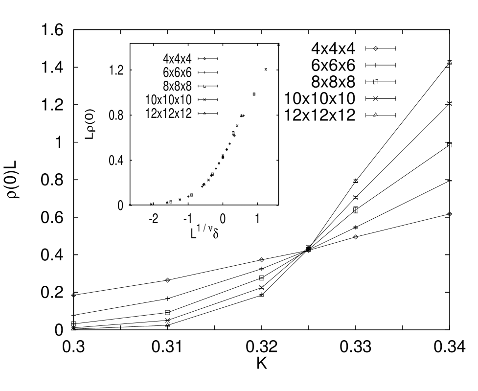
FIG. 4.: The stiffness $\rho(0)L$ at the tip of the lobe ($\Delta=0.2$, $\mu=1.0$). The aspect ratio is constant for $z=1$, the insert shows a scaling plot with $K_{c}=0.325$ and $\nu=0.7$.

We fix $\mu=1$ and vary $K$. Coming from the SF-phase we first analyze the finite size scaling behavior [7] of the superfluid stiffness

$$\rho=\frac{1}{L_{\tau}}[\langle n_{x}^{2}\rangle]_{av}\sim L^{-(d+z-2)}\,\tilde{\rho}(L^{1/\nu}\delta,L_{\tau}/L^{z})\;,$$ (8)

with $n_{x}=1/L\sum_{(i,t)}J^{x}_{(i,t)}$ the winding number. Since we do not know the dynamical exponent $z$ we hypothesized $z=2$ (as for the generic case) and $z=1$ (as in the pure ($\Delta=0$) case). For both we performed runs with constant aspect ration $L_{\tau}/L^{z}$, and it turned out that for $z=1$ the best data collapse could be obtained and that only this value is also compatible with the correlation function results discussed below. In fig. 4 we show our results for $z=1$, where one gets a clear intersection point of $L\rho$ at $K_{c}^{\prime}=0.325\pm 0.002$. This value is very close to the corresponding value for the pure case $K_{c}^{\prime\rm pure}=0.333\pm 0.003$ [18] and indicates that the tip of the lobe depends very weakly on the disorder strength or is even independent of it over some range [12]. In the latter case the critical exponent $\nu$ might escape the inequality $\nu\geq 2/d$ [22] at this special multicritical point [12, 23], since then variation of the disorder cannot trigger the transition as required in [22]. Indeed, the insert of fig. 4 shows a scaling plot which yields $\nu=0.7\pm 0.1<2/d=1$, which agrees well with the pure value (see below). These results yield a consistent picture, nevertheless we should mention that one cannot strictly exclude the possibility that our data are not yet in the asymptotic scaling regime and the exponent $\nu$ we estimate is only an effective exponent for small length scales.

From the data for the imaginary time correlation function $C_{i}(t)$ and the spatial correlation function $C_{x}(r)=[\langle\exp\{-\frac{1}{K}\sum_{x=1}^{r}(1/2+J^{x}_{i+x\hat{e}_{x},t})\}\rangle]_{av}$ shown in fig. 5, we get firm support for $z=1$: The ratio of the decay exponents $y_{x}$ and $y_{\tau}$ for $C_{x}$ and $C_{+}(\tau)=[C_{i}^{+}(\tau)]_{\rm av}$, respectively should equal $z$ and we find $y_{x}/y_{\tau}\approx 1.0(1)$, roughly independent of how we scale $L_{\tau}$ with $L$. From $y_{x}=d+z-2+\eta$ we get $\eta=0.1\pm 0.1$.

FIG. 5.: The correlation functions $C_{x}(r)$ and $C_{+}(\tau)$ for system size 10x10x10 at the tip of the lobe ($K_{c}$=0.325, $\Delta$=0.2, $\mu$=1.0). The dotted lines are least square fits to $C_{x}(r)$=$a(r^{y_{x}}$+$(L$–$r)^{y_{x}})$ and $C_{+}(\tau)$=$a^{\prime}(\tau^{y_{\tau}}$+$(L_{\tau}$–$\tau)^{y_{\tau}})$, which gives $y_{x}$=–1.11 and $y_{\tau}$=–1.08, i.e. $z$=$y_{x}/y_{\tau}$=1.0. The insert shows the compressibility $\kappa$ for $\Delta$=0.2, $\mu$=1.0.

Finally the insert of fig. 5 shows the compressibility at the above studied transition, and we observe that it vanishes here, too. In particular the data scale well according to $\kappa=L^{-1}\tilde{\kappa}(L^{1/\nu}\delta)$ for systems with $L=L_{\tau}$, i.e. constant aspect ratio for $z=1$. Hence, for weak disorder ($\Delta\leq 0.2$) we find at the tip of the lobe a direct SF to MI transition possibly within the same universality class as the pure model, since our estimates for $z$, $\eta$ and $\nu$ are numerically indistinguishable from the values for the the pure XY model in 3d, which are $z=1$, $\eta=0.033(4)$ and $\nu=0.669(2)$ [24].

As one can see from fig. 4 and the insert of fig. 5 there is no sign of a first order transition at the tip of the lobe, as has been suggested in [11]. Moreover, our conclusion disagrees with the mean-field prediction [2] of an intervening BG phase between MI and SF phase at the tip of the lobe for weak disorder. For stronger disorder the scenario might change: for instance at $\Delta=0.4$ we estimate $z\approx 0.4$, which is possibly only an effective exponent and the compressibility does not vanish immediately below the transition from the SF phase. This indicates the existence of a threshold value for the disorder strength: only above this threshold the mean-field prediction might be correct [10, 12].

To conclude, we have shown in this letter that the Bose glass phase in the disordered boson Hubbard model and the Griffiths phase in random transverse Ising models are closely related and that the gapless low energy excitations are fully localized in the BG phase. Moreover, we presented evidence that the transition for commensurate boson densities is directly from a Mott insulating phase to a superfluid phase for weak disorder. The critical exponents we estimate for this special multicritical point are different from those at the generic BG-SG transition at incommensurate boson densities and agree with those for the pure three-dimensional XY model. This suggests that the latter and the tip of the lobe at weak disorder are within the same universality class. Renormalization group and scaling arguments put forward in [12] give strong support to this scenario.

We thank F. Pazmandi, G. T. Zimanyi and A. P. Young for intersting and helpful discussions. This work was supported by the Deutsche Forschungsgemeinschaft (DFG).

REFERENCES

- [1] M. P. A. Fisher, Phys. Rev. Lett. 65, 923 (1990).
- [2] M. P. A. Fisher, P. B. Weichman, G. Grinstein and D. S. Fisher, Phys. Rev. B. 40, 546 (1988).
- [3] Y. Liu et al., Phys. Rev. Lett. 67, 2068 (1991); M. A. Palaanen, A. F. Hebard and R. R. Ruel, Phys. Rev. Lett. 69, 1604 (1992);
- [4] P. A. Crowell, F. W. Van Keuls and J. D. Reppy, Phys. Rev. Lett. 75, 1106 (1995); P. A. Crowell et al., Phys. Rev. B 51, 12721 (1995).
- [5] R. T. Scalettar, G. G. Batrouni and G. T. Zimanyi, Phys. Rev. Lett. 66, 3144 (1991).
- [6] W. Krauth, N. Trivedi and D. Ceperley, Phys. Rev. Lett. 67, 2307 (1991).
- [7] E. S. Sørensen, M. Wallin, S. M. Girvin and A. P Young, Phys. Rev. Lett. 69, 828 (1992); M. Wallin, E. S. Sørensen, S. M. Girvin and A. P. Young, Phys. Rev. B 49, 12115 (1994).
- [8] M. Makivić, N. Trivedi and S. Ullah, Phys. Rev. Lett. 71, 2307 (1993).
- [9] S. Zhang, N. Kawashima, J. Carlson and J. E. Gubernatis, Phys. Rev. Lett. 74, 1500 (1995).
- [10] K. G. Singh and D. Rokshar, Phys. Rev. B 46, 3002 (1992).
- [11] J. K. Freericks and H. Monien, Phys. Rev. B 53 (1996).
- [12] F. Pazmandi, G. T. Zimanyi, R. Scalettar, to be published.
- [13] R. B. Griffiths, Phys. Rev. Lett. 23, 17 (1969); B. McCoy, Phys. Rev. Lett. 23, 383 (1969).
- [14] D. S. Fisher, Phys. Rev. Lett. 69, 534 (1992); Phys. Rev. B 51, 6411 (1995).
- [15] A. P. Young and H. Rieger, Phys. Rev. B 53, 8486 (1996).
- [16] H. Rieger and A. P. Young, Phys. Rev. B 54, 3329 (1996).
- [17] M. Guo, R. N. Bhatt and D. A. Huse, Phys. Rev. B 54, 3323 (1996).
- [18] J. Kisker and H. Rieger, to be published.
- [19] J. Villain, J. Phys. 36, 581 (1975).
- [20] The dynamical exponent that parametrizes the Griffiths– or Boseglas phase as in eq. (4) has its origin in purely local effects, whereas the critical exponent describes global, collective excitations at the critical point.
- [21] F. Pazmandi, G. T. Zimanyi and R. Scalettar, Phys. Rev. Lett. 75, 1356 (1995).
- [22] J. T. Chayes, L. Chayes, D. S. Fisher and T. Spencer, Phys. Rev. Lett. 57, 2999 (1986).
- [23] M. E. Fisher and R. R. P. Singh, Phys. Rev. Lett. 60, 548 (1988).
- [24] J. C. Le Guillou, J. Zinn-Justin, Phys. Rev. B 21, 3976(1980).